
Model Development to Study Uncertainties in Electric Arc Furnace Plants to Improve Their Economic and Environmental Performance


Abstract
1. Introduction
2. Model Description
2.1. Simulation of a Charge Program
2.1.1. Scrap Simulation
2.1.2. Charge Program Simulation
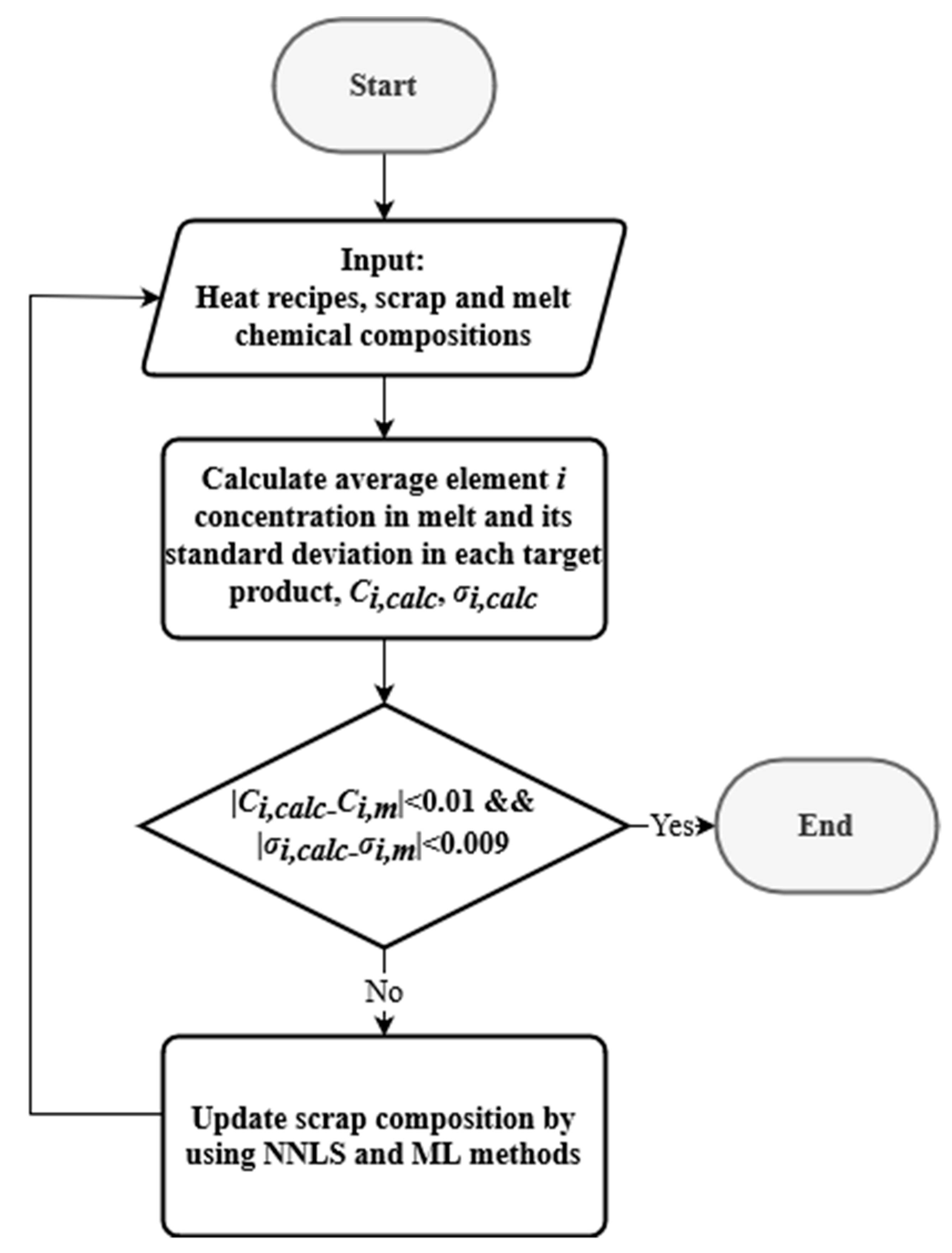
2.2. Backward Estimation of Scrap Composition
2.2.1. Uncertainties in Scrap Chemical Composition
2.2.2. Uncertainties in Scrap Chemical Composition and Weighing
2.2.3. Uncertainties in Scrap Chemical Composition and Element Distribution Factors
3. Model Validation and Application
4. Results and Discussion
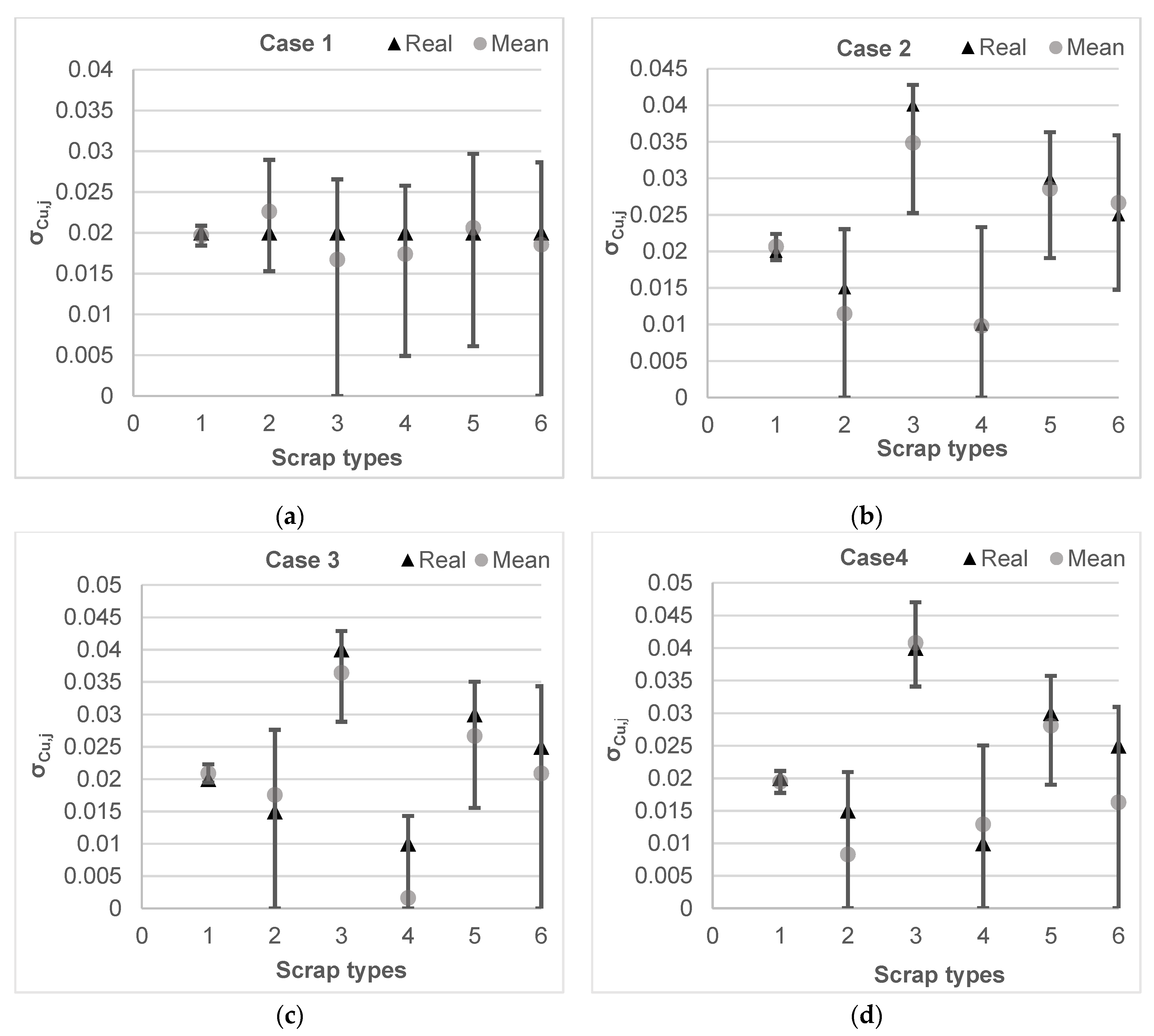
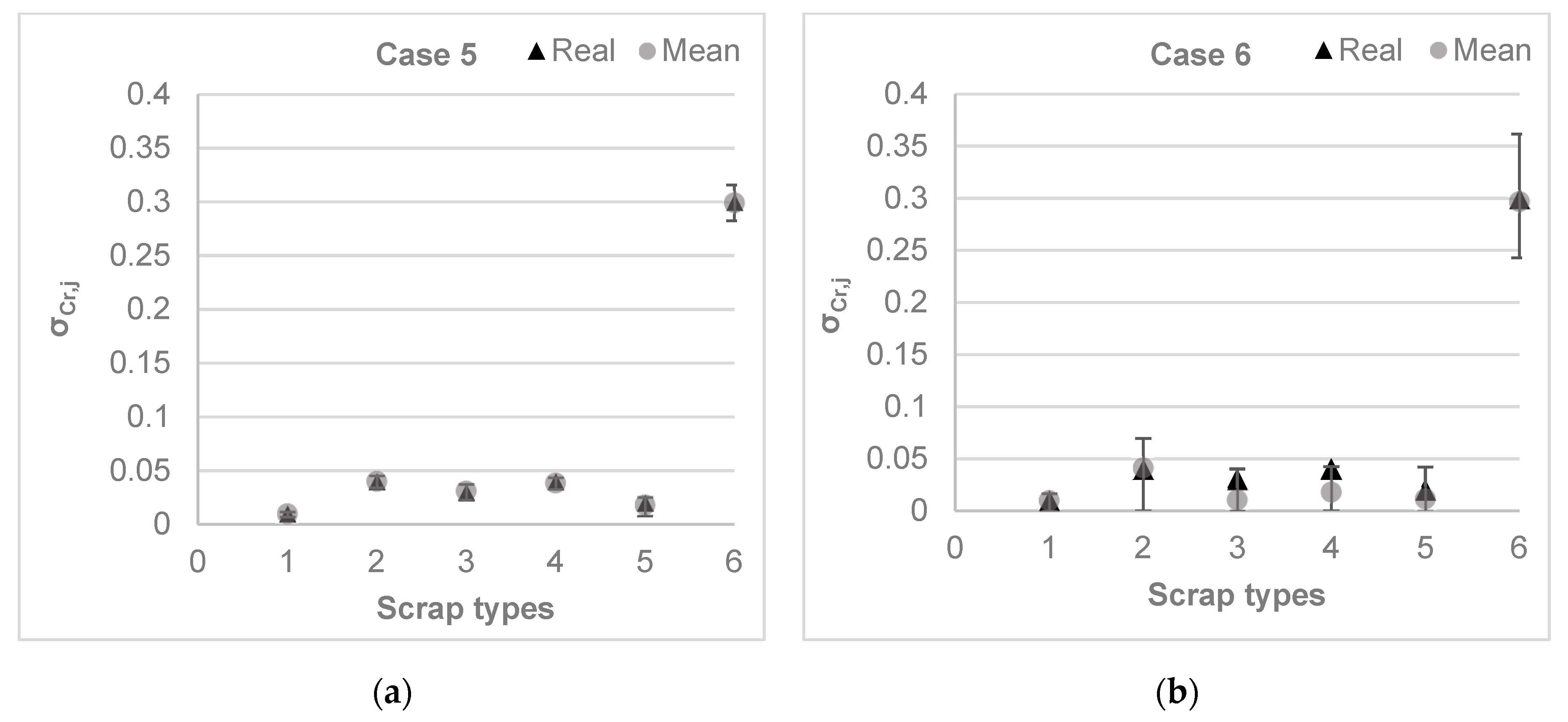
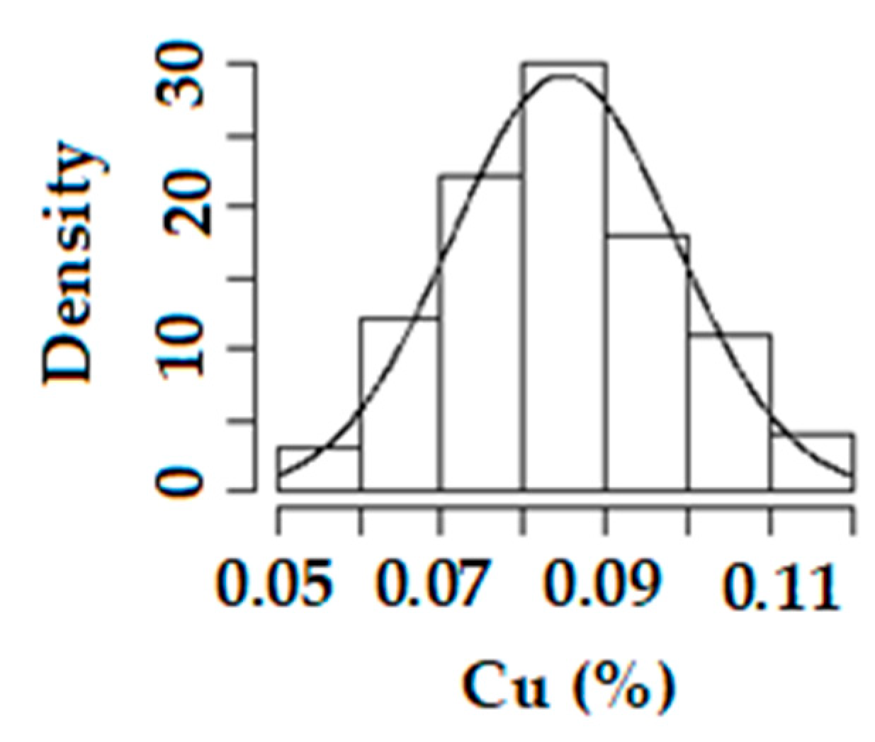
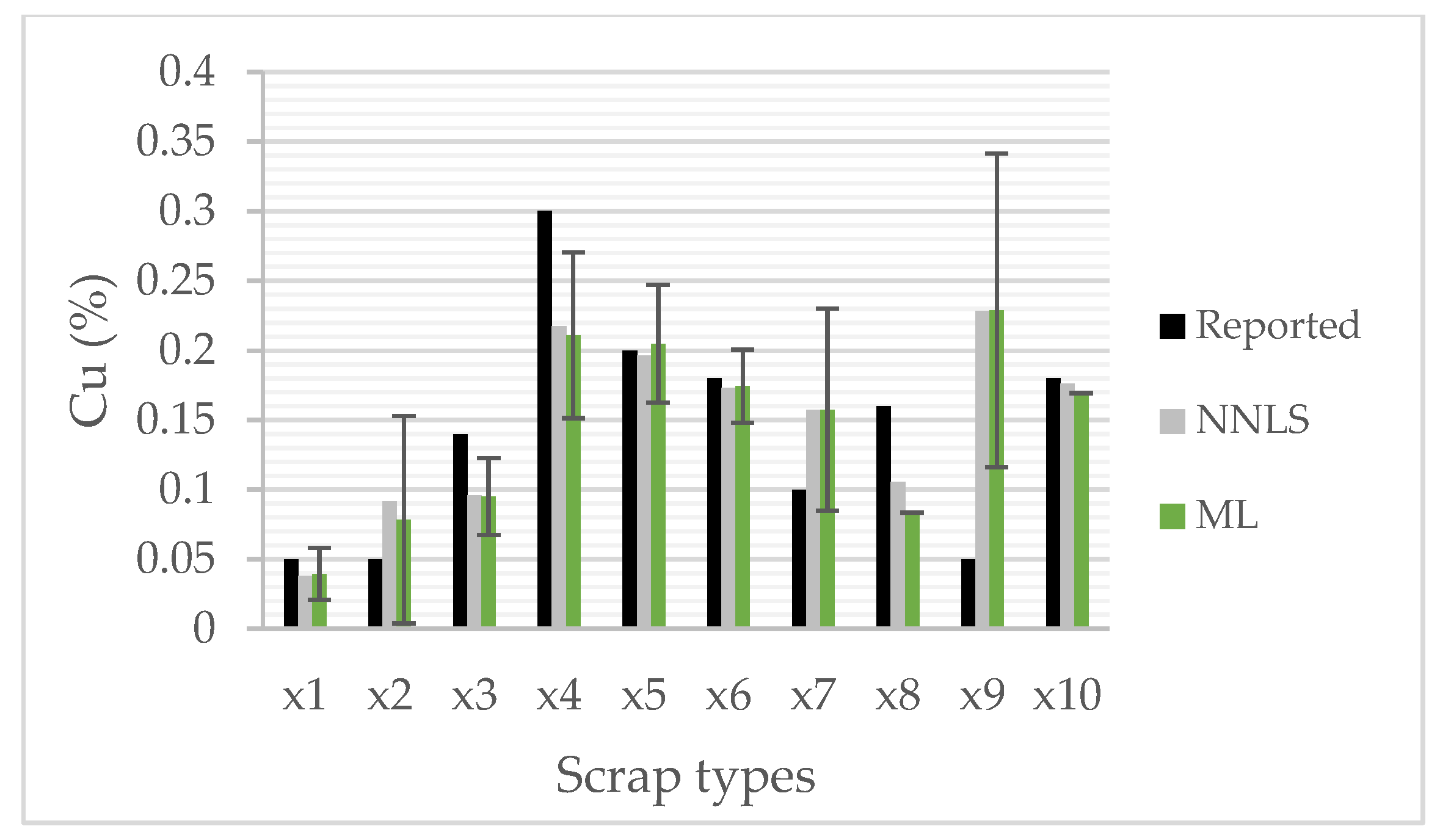
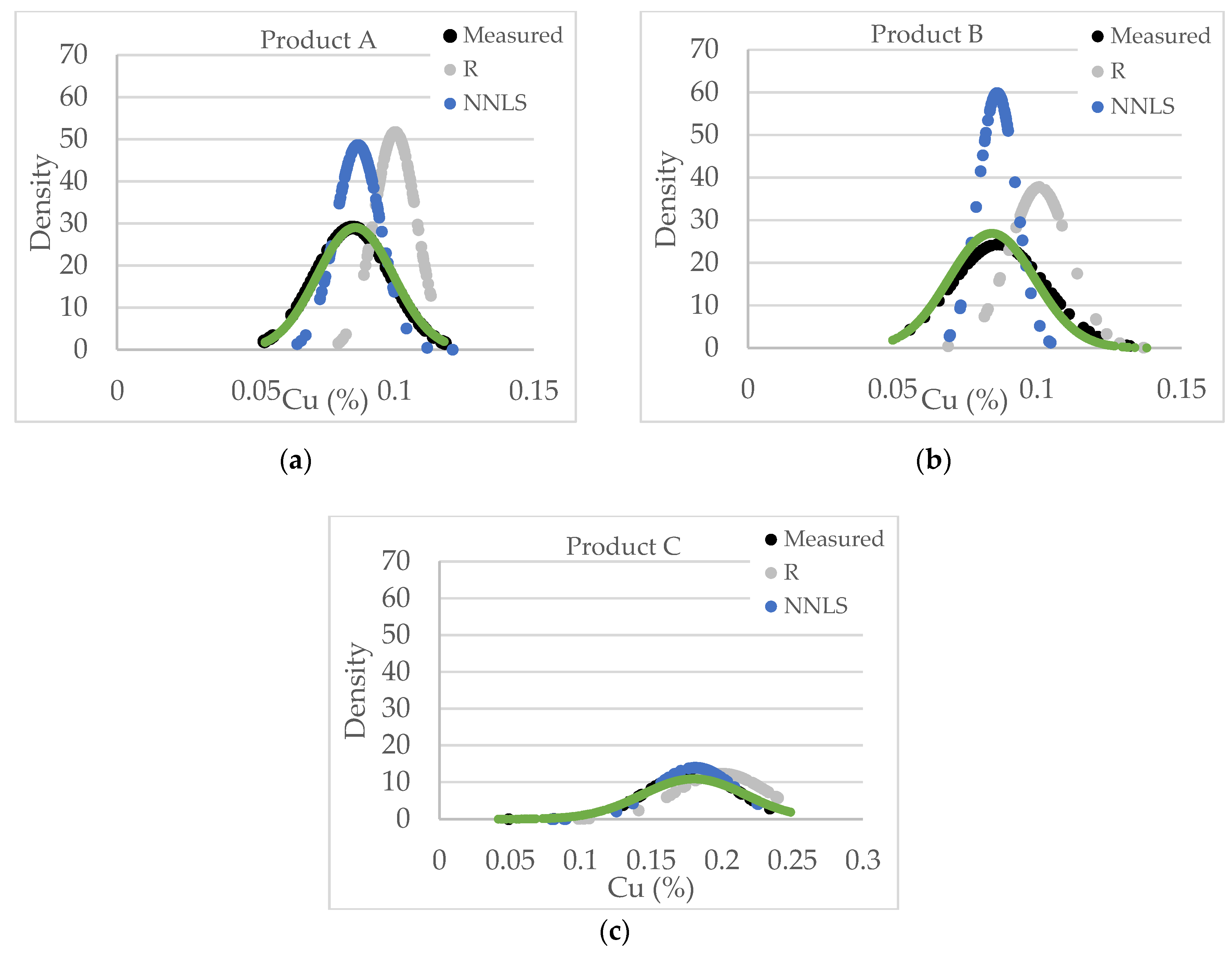
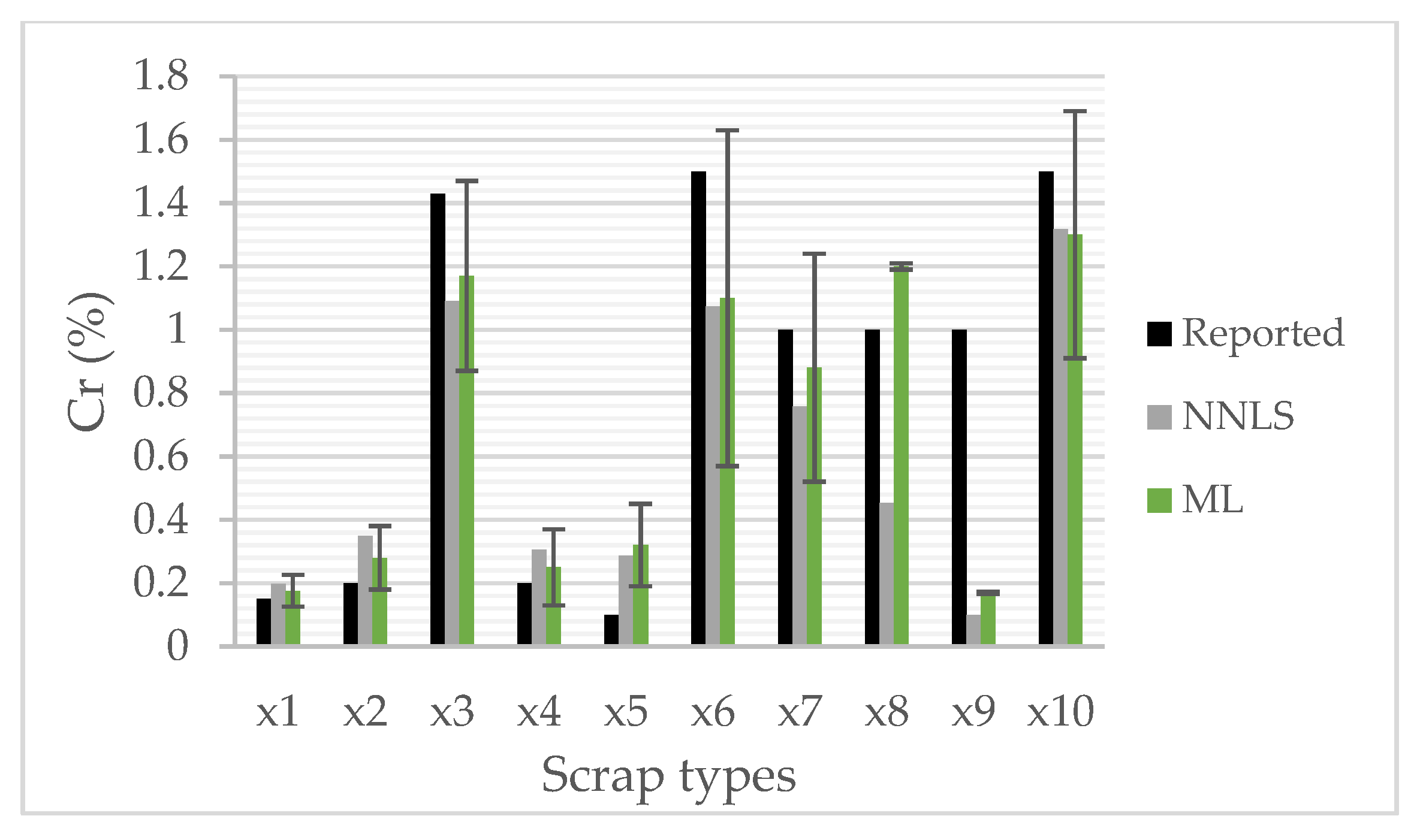
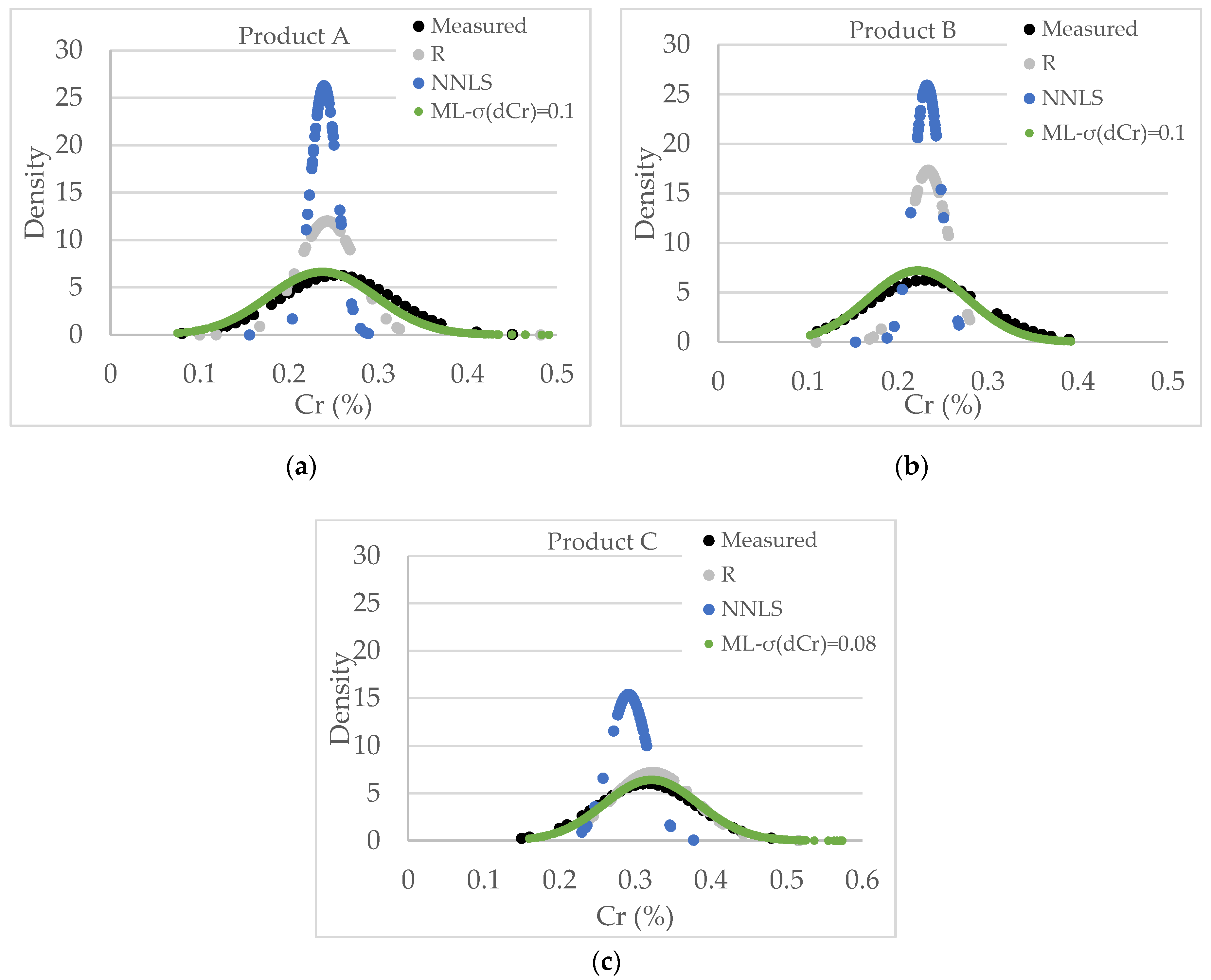
4.1. Model Validations Results
4.2. Model Application Results
4.3. Use of the Model
5. Conclusions
Author Contributions
Funding
Acknowledgments
Conflicts of Interest
Appendix A

| Furnace capacity (tonne) | 100 |
| Maximum concentration of copper in target product (%) | 0.2 |
| Scrap Price (USD/kg) | 0.23 |
| Scrap upstream carbon footprint (kg CO2eq/kg) | 0.007 |
| Pig iron price (USD/kg) | 0.41 |
| Pig iron upstream carbon footprint (kg CO2eq/kg) | 1.85 |
References
- Bekker, J.; Craig, I. Modeling and Simulation of an Electric Arc Furnace. ISIJ Int. 1999, 32, 23–32. [Google Scholar] [CrossRef]
- Gaustad, G.; Preston, L.; Kirchain, R. Modeling Methods for Managing Raw Material Compositional Uncertainty in Alloy Production. Resour. Conserv. Recycl. 2007, 52, 180–207. [Google Scholar] [CrossRef]
- Badr, K.; Kirschen, M.; Cappel, J. Chemical Energy and Bottom Stirring Systems-Cost Effective Solutions for a Better Performing EAF. In Proceedings of the METEC InSteelCon, Düsseldorf, Germany, 27 June–1 July 2011. [Google Scholar]
- MacRosty, R.; Swartz, C. Dynamic Modeling of an Industrial Electric Arc Furnace. Ind. Eng. Chem. Res. 2005, 44, 8067–8083. [Google Scholar] [CrossRef]
- Logar, V.; Dovžan, D.; Škrjanc, I. Modeling and Validation of an Electric Arc Furnace: Part 1, Heat and Mass Transfer. ISIJ Int. 2012, 52, 402–412. [Google Scholar] [CrossRef]
- Lahdelma, R.; Hakonen, H.; Ikäheimo, J. AMRO—Adaptive Metallurgical Raw Material Optimization. In Proceedings of the IFORS’99, Beijing, China, 16–20 August 1999. [Google Scholar]
- Rong, A.; Lahdelma, R. Fuzzy Chance Constrained Linear Programming Model for Optimizing the Scrap Charge in Steel Production. Eur. J. Oper. Res. 2008, 186, 953–964. [Google Scholar] [CrossRef]
- Gauffin, A.; Tilliander, A.; Jönsson, P.G. Alloy content in steel scrap by use of random sampling analysis and its impact on the Electric arc furnace. In Proceedings of the Shechtman International Symposium, Cancun, Mexico, 29 June–4 July 2014. [Google Scholar]
- Birat, J.P.; Coq, X.L.; Russo, P. Quality of Heavy Market Scrap: Development of New and Simple Methods for Quality Assessment and Quality Improvement; Technical Steel Research; European Commission: Brussels, Belgium, 2002. [Google Scholar]
- Sandberg, E.; Lennox, B.; Undvall, P. Scrap Management by Statistical Evaluation of EAF Process Data. Control Eng. Pract. 2007, 15, 1063–1075. [Google Scholar] [CrossRef]
- Savov, L.; Volkova, E.; Janke, D. Copper and Tin in Steel Scrap Recycling. Mater. Geoenviron. 2003, 50, 627–640. [Google Scholar]
- Gyllenram, R.; Westerberg, O. The impact of scrap upgrading on EAF production cost and performance. Stahl Eisen 2016, 1, 31–36. [Google Scholar]
- RAWMATMIX® Manual System, Version 2.16; Kobolde & Partners AB: Stockholm, Sweden, 2020.
- Arzpeyma, N.; Gyllenram, R.; Jönsson, P.G. Development of a Mass and Energy Balance Model and its Application for HBI Charged EAFs. Metals 2020, 10, 311. [Google Scholar] [CrossRef]
- Lawson, C.L.; Hanson, R.J. Solving Least Squares Problems; Society for Industrial and Applied Mathematics: Philadelphia, PA, USA, 1995. [Google Scholar]
- Rossi, R.J. Mathematical Statistics: An Introduction to Likelihood Based Inference; John Wiley & Sons: New York, NY, USA, 2018. [Google Scholar]
- R. C. Team. A Language and Environment for Statistical Computing. R Foundation for Statistical Computing. Vienna, Austria. 2020. Available online: http://www.R-project.org/ (accessed on 2020).
- Nash, J.C. On Best Practice Optimization Methods in R. J. Stat. Softw. 2014, 20, 1–14. [Google Scholar]


| Scenario | Actual Cu in Scrap (%) | Assumed Cu in Scrap (%) | Scrap Amount (kg) | Pig Iron Amount (kg) | Material Cost (USD/tm) | Carbon Footprint Scope 3 (kgCO2eq/tm) |
|---|---|---|---|---|---|---|
| 1 | 0.1 | 0.1 | 102,301 | 0 | 238 | 9 |
| 2 | 0.1 | 0.3 | 68,027 | 34,561 | 300 | 647 |
| j | 1 | 2 | 3 | 4 | 5 | 6 |
|---|---|---|---|---|---|---|
| CCu,j (%) | 0.05 | 0.05 | 0.14 | 0.3 | 0.2 | 0.05 |
| CCr,j (%) | 0.15 | 0.2 | 1.43 | 0.2 | 0.1 | 1 |
| Case | ||||||||
|---|---|---|---|---|---|---|---|---|
| 1 | 0.02 | 0.02 | 0.02 | 0.02 | 0.02 | 0.02 | 0 | 0 |
| 2 | 0.02 | 0.015 | 0.04 | 0.01 | 0.03 | 0.025 | 0 | 0 |
| 3 | 0.02 | 0.015 | 0.04 | 0.01 | 0.03 | 0.025 | 10 | 0 |
| 4 | 0.02 | 0.015 | 0.04 | 0.01 | 0.03 | 0.025 | 50 | 0 |
| Case | ||||||||
| 5 | 0.01 | 0.04 | 0.03 | 0.04 | 0.02 | 0.3 | 0 | 0 |
| 6 | 0.01 | 0.04 | 0.03 | 0.04 | 0.02 | 0.3 | 0 | 0.05 |
| Cases | x1 | x2 | x3 | x4 | x5 | x6 |
|---|---|---|---|---|---|---|
| 1 | 0.049 | 0.051 | 0.142 | 0.302 | 0.201 | 0.042 |
| 2 | 0.048 | 0.048 | 0.145 | 0.303 | 0.202 | 0.055 |
| 3 | 0.049 | 0.049 | 0.142 | 0.301 | 0.204 | 0.046 |
| 4 | 0.049 | 0.049 | 0.140 | 0.302 | 0.199 | 0.065 |
| 5 | 0.151 | 0.195 | 1.427 | 0.196 | 0.104 | 0.993 |
| 6 | 0.147 | 0.204 | 1.435 | 0.209 | 0.104 | 0.943 |
| Cases | Variable | x1 | x2 | x3 | x4 | x5 | x6 |
|---|---|---|---|---|---|---|---|
| 1 | 0.05 | 0.051 | 0.139 | 0.303 | 0.201 | 0.043 | |
| 0.02 | 0.023 | 0.017 | 0.017 | 0.021 | 0.019 | ||
| 2 | 0.048 | 0.048 | 0.145 | 0.303 | 0.201 | 0.055 | |
| 0.021 | 0.011 | 0.035 | 0.010 | 0.029 | 0.027 | ||
| 3 | 0.049 | 0.052 | 0.143 | 0.302 | 0.204 | 0.046 | |
| 0.021 | 0.018 | 0.036 | 0.002 | 0.027 | 0.021 | ||
| 4 | 0.050 | 0.048 | 0.141 | 0.301 | 0.197 | 0.064 | |
| 0.019 | 0.008 | 0.041 | 0.013 | 0.028 | 0.016 | ||
| 5 | 0.151 | 0.195 | 1.426 | 0.196 | 0.103 | 1.011 | |
| 0.01 | 0.04 | 0.031 | 0.038 | 0.018 | 0.299 | ||
| 6 | 0.150 | 0.202 | 1.429 | 0.204 | 0.097 | 0.994 | |
| 0.010 | 0.041 | 0.011 | 0.018 | 0.012 | 0.297 |
Publisher’s Note: MDPI stays neutral with regard to jurisdictional claims in published maps and institutional affiliations. |
© 2021 by the authors. Licensee MDPI, Basel, Switzerland. This article is an open access article distributed under the terms and conditions of the Creative Commons Attribution (CC BY) license (https://creativecommons.org/licenses/by/4.0/).
Share and Cite
Arzpeyma, N.; Alam, M.; Gyllenram, R.; Jönsson, P.G. Model Development to Study Uncertainties in Electric Arc Furnace Plants to Improve Their Economic and Environmental Performance. Metals 2021, 11, 892. https://doi.org/10.3390/met11060892
Arzpeyma N, Alam M, Gyllenram R, Jönsson PG. Model Development to Study Uncertainties in Electric Arc Furnace Plants to Improve Their Economic and Environmental Performance. Metals. 2021; 11(6):892. https://doi.org/10.3390/met11060892
Chicago/Turabian StyleArzpeyma, Niloofar, Moudud Alam, Rutger Gyllenram, and Pär G. Jönsson. 2021. "Model Development to Study Uncertainties in Electric Arc Furnace Plants to Improve Their Economic and Environmental Performance" Metals 11, no. 6: 892. https://doi.org/10.3390/met11060892
APA StyleArzpeyma, N., Alam, M., Gyllenram, R., & Jönsson, P. G. (2021). Model Development to Study Uncertainties in Electric Arc Furnace Plants to Improve Their Economic and Environmental Performance. Metals, 11(6), 892. https://doi.org/10.3390/met11060892