Abstract
The aim of this study is to exhibit the mutual connection between surface and in depth hardness values in the case of surface-treated metal samples with inhomogeneous hardness distribution in the surface layer. The reason for surface treatments of metal alloys is most commonly to increase the hardness and wear resistance at the surface. Case depth, as a result of surface treatment and the in-depth hardness distribution, can be determined by measuring the hardness of a section perpendicular to the treated surface and by metallographic examination. The result of heat treatment can also be checked rapidly by surface hardness testing. Surface hardness carries only indirect information regarding case depth and hardness distribution. Surface and cross-sectional hardness can be related to the mathematical modeling of the plastic zone developing in the indentation process. The mathematical model applied in this study allows the conversion of the surface hardness function into the in-depth hardness function and vice-versa. The calculation method presented was validated by analyzing the hardness data of nitrocarburized samples of various case depths. The validation result proves that cross-sectional hardness distribution can be adequately estimated by surface hardness data in the case of a surface layer with monotonically decreasing hardness distribution.
1. Introduction
The most widely used method of grading the hardened or coated surface layers of metals is by evaluating the hardness values obtained using indentation hardness tests (Vickers-ISO 6507, Rockwell-ISO 6508). The surface layer can be graded by two important indicators that need to be determined or estimated. One is surface hardness, which is of paramount importance, as it greatly influences wear on an operating machine part. Determining the surface hardness is not a trivial task in itself, as the measured hardness depends on the procedure used and on the load. This is because the measured surface hardness depends not only on the hardness of the surface but also on the hardness of the material under the surface layer, which is usually softer. Hardness of the surface Hs is a function of the load; the higher the load, the lower the surface hardness. At the same time, as Figure 1a shows, Hs can also be considered a function of indentation depth (F1 < F2 < F3 < F4); hereinafter, the term surface hardness function is used for the latter (Hs = Hs(h)). The other indicator is the thickness of the surface layer, which can be determined by a destructive method on a section perpendicular to the surface of the sample (a series of hardness tests executed with small, usually identical loads). The Hd discreet hardness values determined at given distances from the surface are considered to be elements of the continuous hardness function, usually monotonously decreasing from the surface, as shown in Figure 1b (Hd = Hd(x)). In this way, the relationship between the distance from the surface and hardness, that is, the in-depth hardness function, can be approximated. With the use of this function, layer thickness can be determined based on the relevant standards or regulations. Metallurgical tests are also performed on the section perpendicular to the surface, as surface treatments usually result in characteristic changes in the microstructure.
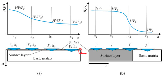
Figure 1.
Interpretation of the Hs surface and the Hd in-depth hardness function. (a) Surface; (b) in-depth.
The surface hardness Hs(h) and in-depth hardness Hd(x) functions are related, of course, as the hardness of the same surface layer is investigated with hardness tests in different directions and positions. Surface hardness testing with small loads provides information about the upper part of the layer. However, this information represents an average mechanical behavior of an area near the surface, since however small the load is, it causes an h indentation depth, which is greater than zero. Measured hardness is influenced not only by the surface material of thickness h but also by the material around and under the indentation. When determining the hardness of the layer with a small load, we have to take into account the indentation size effect (ISE), as with small loads, hardness may vary as a function of the load [1,2]. In this paper, we do not take ISE into account, considering that even with the smallest load used (1.962 N, HV0.2), the indentation depth h was typically greater than 2 μm. The greater the load in hardness testing, the less the result describes the hardness of the outer layer since the influence of the supporting layer and the basic matrix also grows. The following questions thus arise: what does a surface hardness actually describe, and how can surface hardness results be interpreted in the case of an inhomogeneous hardness distribution?
The main aim of this research is to study whether the mechanical properties of a surface layer, with inhomogeneous hardness distribution, can be estimated based on its surface hardness testing.
2. Composite Hardness and Its Interpretation
Analyzing the information content of surface hardness has become important, as thin surface coatings (e.g., PVD, physical vapor deposition) have become more widely used. In these cases, determining the hardness of the surface film carries much uncertainty, as the hardness of the substrate also influences the measurement results. At this time, mathematical models, which interpreted surface hardness as so-called composite hardness, were developed. The measured composite hardness is a combination of substrate and surface film hardness. These models allow the estimation of the hardness surface film from the measured composite hardness if the hardness of the substrate is known.
Bückle [1] was the first to propose a method to calculate composite hardness using the hardness of the substrate and the film. Jönsson and Hogmark’s [3] model works on similar principles. It uses simple surface geometrical approach to separate the contribution of the substrate and the coating to the measured hardness, and the resultant hardness was derived from the relative projected sizes of the load-supporting areas under the indenter. Burnett and Rickerby [4] published a novel method to determine composite hardness, which takes into account the elastoplastic behavior of the material under the indenter. They applied a volumetric mechanical model of indentation, which is based on the analogy with the expansion of a spherical cavity due to internal pressure. The theoretical background of this approach and its adaptation to indentation hardness testing have been known since the 1970s [5,6,7]. Burnett et al. considered the volumetric ratio of film and substrate in the plastic zone in the calculation of composite hardness; therefore, this approach takes into account the plastic strain energy ratio of the coating and the matrix in the indentation process. Iost compared the Jönsson and Hogmark model and its improved version (Korsunsky model) [8,9] with the modified Puchi-Cabrera [10] procedure and applied them to determine the actual hardness of thin layers [11]. Coorevits and Mejias developed a method to determine in-depth hardness distribution, also based on the work of Jönnson and Hogmark [12].
Khalay [13] developed an artificial neural network-based model (ANNs) to predict the layer thickness of pre-nitrided steels. In another work, Khalaj and Pouraliakbara [14] modelled layer thickness of treated coating by gene expression programming (GEP). A lot of research has dealt with the relationship between the plastic zone size and plastic depth during indentation. The fundamental expression of the relationship between the radius of the plastic deformation zone and the residual indentation depth was written by Lawn et al. [15]. Giannakopoulos and Suresh [16,17] found that the radius of the plastic deformation zone can be expressed in terms of applied load and yield strength. Nayebi et al. [18,19] analyzed heat-treated tool steels with a gradient in hardness (yield strength), utilizing instrumented indentation and finite element models in order to predict the hardness versus depth profile of a heat-treated steel. Chen and Bull [20] studied the relationship between the plastic zone radius and residual indentation depth, which was examined by using finite element analysis. Klecka et al. [21] showed a rapid novel method to predict the gradients produced during surface heat treatment, which consisted of only a series of indentations at increasing loads on the sample surface requiring only a hardness tester and minimal sample preparation.
Detailed knowledge of this topic is also important since thin coatings have a great effect on the material’s performance or lifetime. There is a correlation between the microstructure and the mechanical properties (hardness and elastic modulus), impact resistance, and tribological performance of different systems.
For example, mono- and multi-layers have a very big effect on the lifetime and cutting ability of cutting tools [22,23,24,25]. The carbonized and nitrided surfaces also have a great effect to the microstructural, hardness, tribological, and corrosion behavior of parts [26,27,28,29].
In this paper, following Burnett’s approach, composite hardness is interpreted as a volumetric characteristic feature. The calculation of composite hardness is based on the volume of the hemispherical plastic zone, as shown in Figure 2 [4]. The applicability of this approach in the case of a Vickers-type indenter is also proved by Mata’s finite element computational results [30].
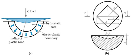
Figure 2.
The plastic zone under the indenter (a) and its sections (b).
According to the theory describing elastoplastic behavior during hardness testing (expansion of a spherical cavity caused by internal pressure), the relationship between radius b of the hemisphere, which is the boundary surface of elastic–plastic deformation zones, and the half-diagonal a of the Vickers indentation (a = d/2) is
where E is the elastic modulus (GPa), Hs is surface hardness (GPa), p is a constant between 2 and 3 (in this study, p = 3), and φ is the indenter semi-angle (148°/2 = 74°). Equation (1) is of paramount importance in practice because it describes the connection between indentation size and the radius of the plastic zone. Due to the geometrical connection between diagonal d and depth h of the indentation, b, the radius of the plastic zone can be interpreted directly as a function of h indentation depth (b = b(h)).
Burnett’s model was improved by Ichimura and applied to evaluate PVD layers of duplex-coated tool steels [31,32]. In order to take into account the effect of non-homogenous hardness distribution in the substrate, he divided the volume of the radius b hemisphere of the plastic zone into n + 1 spherical segments along planes parallel to the surface. Ichimura then calculated composite hardness in the following way:
where Vf and Hf are the volume and hardness of the surface film, respectively; Vi and Hi are the volume and characteristic hardness of the ith spherical segment under the surface, respectively; and V0 is the volume of the plastic zone of radius b. If the surface film is neglected, then Equation (2) can be written as Equation (3) based on the generalization shown in Figure 3. If the in-depth hardness distribution is appropriately known, the surface hardness belonging to an h indentation depth can be estimated with Equations (1) and (3).
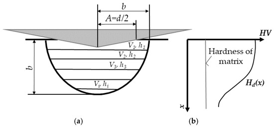
Figure 3.
Interpreting composite hardness (a) and the hardness distribution of the layer (b).
In Equation (3), i = 1 is the spherical segment in contact with the surface.
3. Connection between Surface and In-Depth Hardness Functions
The in-depth hardness distribution of surface-treated layers Hd(x) is usually monotonously decreasing from the surface. This is logical, since the goal of surface treatment (i.e., carburizing, surface hardening, or nitriding) is to increase hardness and wear-resistance. In some special cases, the maximum hardness is not on the surface (e.g., due to retained austenite or decarburization), but in most cases, there is little difference between surface hardness and maximum hardness and their location; therefore, a monotonously decreasing function can be assumed.
The hardness in the depth direction (from the surface to the base matrix) can be considered a continuous function in the case of hardening and surface hardening. The nitrided surface may also contain a very hard, thin compound layer with a sharp interface to the diffusion zone. In this case, the continuity of the hardness function can only be considered to be true for the diffusion range. In the case of a compound nitride layer or, e.g., PVD coating, assuming a stepwise function is reasonable. The methodology of the present study can be considered to be valid for surface treatment resulting in a continuous and monotonically decreasing in-depth hardness function (e.g., case hardening, surface hardening, or nitriding without a compound layer).
The best way to approximate in-depth hardness distribution is with a function, as this makes numerical calculations much easier. Based on preliminary calculations and the physical meaning of the parameters, the following sigmoid function was chosen to describe the in-depth hardness distribution:
where A1 is the upper and A2 is the lower bound of the hardness function; x0 is the x coordinate of the point of inflection; and dx is a time constant describing the stretching of the function along the x axis.
3.1. Calculating the Surface Hardness Function from the In-Depth Hardness Distribution
From the in-depth hardness distribution approximated with Equation (4), surface hardness can be determined by Equations (1) and (3) for predefined indentation depths. Let us suppose that the in-depth hardness function is known and hardness distribution is defined by the following parameters: A1 = 1100 HV, A2 = 500 HV, x0 = 100 μm, dx = 12.5 μm. The x0/dx ratio is 8. In this case, Figure 4 shows the sigmoid function.
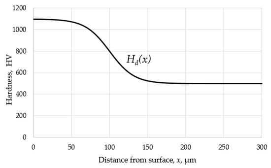
Figure 4.
The sigmoid function representing the Hd(x) in-depth hardness distribution.
Let us choose the h indentation depths for which surface hardness has to be determined. Let us define h as a function of indentation diagonal according to the table below (h~d/7 can be considered). The value of h has to fit both the indentation depth range of the Vickers hardness test and the expected layer thickness.
Considering that Equation (1) contains the surface hardness H, which has to be calculated, determining the b plastic zone radius function requires a multi-cycle recursive calculation with the following steps:
- Let us choose H0 as an initial estimated value of the Hs(h) surface hardness function for a given d and h.
- Let us determine b and Hs(h) for all selected h indentation depths. Then, we consider the surface hardness results as the initial values in the next computational cycle.
- If the cycle is repeated several times, the resultant values converge to the final result.
- We subtract the final value from the initial value for each h in the given cycle. If the differences are below a predefined error limit, the final values of the surface hardness series are obtained. Experience shows that a difference of less than 0.01 HV can be attained after 6–8 cycles.
For the sake of simplicity, let us choose an initial hardness of H0 = 500 HV for all indentation depths given in Table 1 and let the error level be 0.01 HV. Table 2 shows the calculated hardness values in the consecutive cycles. It can be seen that the input values (given in cycle 6) and the values calculated in cycle 7 are identical up to two decimal places.

Table 1.
The indentation properties selected for determining the surface hardness.
Table 2.
The results of the recursive calculation in every cycle, HV.
The results in the last column of the table show the surface hardness for the given h indentation depth. The required load can be calculated from the size of the indentation and the hardness, according to the definition of Vickers hardness. Table 3 contains the calculated loads.
Table 3.
Loads belonging to indentation depths.
Since the load can be set as predefined discreet values on hardness testers, it is recommended that the values in Table 3 are converted to common (standard) loads by linear interpolation or extrapolation.
The original (Table 3) and the interpolated indentation depth–hardness pairs (Table 4) are shown together in Figure 5.
Table 4.
Hardness and properties of indentation in the case of common loads.
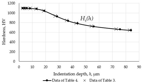
Figure 5.
Relationship of h indentation depth and surface hardness (Hs(h)).
Finally, Figure 6 summarizes the most important results. The starting point is the in-depth (or cross-sectional) hardness distribution. A thick line shows it as a function of x, the distance from the surface (identical to the function in Figure 4). The final result is the surface hardness series shown as a function of h indentation depth, represented by the thin line (same as the function in Figure 5). In the example, a surface indentation of 50 μm deep represents a hardness of 730 HV; that is, a surface hardness of 730 HV is obtained, with a load causing an indentation depth of 50 μm. Figure 6 also shows a function with a dashed line representing the b radius of the plastic zone that belongs to the given Hs(h) = Hs(b) surface hardness (and h). The individual values of surface hardness (thin line) were determined by the use of in-depth hardness values of the hemisphere whose radius is marked with the dashed line. For example, at a point belonging to 730 HV (where the surface hardness testing indentation depth is 50 μm), the radius of the plastic zone is about 370 μm. This means that this point of the surface hardness function was calculated with the use of the volume and hardness of a hemispherical plastic zone of a radius of 370 μm, according to Figure 3.
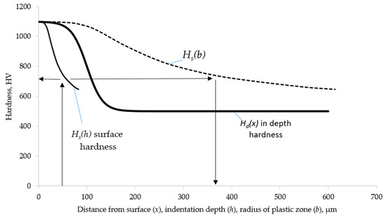
Figure 6.
In-depth and surface hardness function and the radius of the plastic zone.
3.2. Estimating the In-Depth Hardness Distribution from Surface Hardness Values
In this case, the input data series is the measured Hs(h) surface hardness, and the output, the result, is the Hd(x) function, which characterizes in-depth hardness distribution. The calculation of the in-depth hardness distribution from the surface hardness values can be traced back to the inverse calculation described in Section 3.1. In the inverse calculation, the parameters of the in-depth hardness objective function (sigmoid function) are varied in a reasonably chosen range. In each parameter combination, the difference in the calculated and measured value series, or the error function, can be determined (see Equation (5)). We are looking for the parameter combination of Equation (4), which belongs to the minimum value of surface hardness error function. These parameters will represent the Hd(x) in-depth hardness distribution, which approximates surface hardness values with the smallest error in the examined parameter range.
For an efficient solution of the inverse calculation, it is best to narrow down the parameter range. Since the parameters of Equation (4) have a physical meaning, the range to be examined can be specified fairly well if the material and the type of surface treatment are known. Parameter A1 is the maximum value of in-depth hardness distribution. Its expected range can be estimated accurately in the case of commonly used surface treatments. The hardness of the basic matrix, A2, is usually known; therefore, it can be considered a constant. x0 is the distance of the inflexion point of the curve from the surface. It is a free variable, and its range corresponds to the expected layer thickness. dx can be calculated from the x0/dx ratio; this ratio is usually between 2 and 40 for surface layers. The greater the x0/dx ratio is, the more sharply hardness changes in the vicinity of the inflexion point.
4. Materials
The relationship between surface hardness and the hardness distribution was studied on sections perpendicular to the surface of nitrocarburized hot working tool steel samples. The material of the samples was 1.2344 ESR/ESU electroslag remelted, high-purity hot working tool steel (C 0.39%, Cr 5.2%, Mo 1.4%, V 0.95%, Si 1.1%), with fine carbide distribution. This tool steel grade is used for the production of die casting tools, filling chambers, and injection molds for plastic.
The tool steel samples were heat treated according to the specifications of this quality as follows: austenitization in vacuum at 1050 °C; cooling in high-pressure nitrogen; and annealing in a nitrogen atmosphere three times at 530 °C, 600 °C, and 570 °C. After heat treatment, the average hardness of the samples was 50.6 HRc (521 HV). The specimens were nitrocarburized in a cyanide-free salt bath. After preheating at 380 °C for 60 min, the samples were nitrocarburized at 580 °C, for 60, 120, and 480 min for significantly different case depths. The target nitrided case depth was 0.08 mm (60 min), 0.1 mm (120 min), and 0.18 mm (480 min).
After heat treatment, the compound layer was removed chemically; accordingly, the continuous monotonic decreasing nature of the in-depth hardness function can be assumed.
In-depth hardness was measured on polished sections perpendicular to the surface, with a HV0.2 (1.962 N) load, with the Vickers method in steps of 50 μm. Surface hardness was also measured with the Vickers method, with increasing loads. For microhardness tests, loads of 0.2, 0.5, 1, and 2 kgf for macrohardness tests loads of 5, 10, 20, 30, 40, 60, 100, and 120 kgf were used. Hardness was tested with a Zwick 3212 (ZwickRoell GmbH & Co. KG, Ulm, Germany) and a conventional hardness tester. Three series of parallel measurements were performed.
5. Conversion of Surface and In-Depth Hardness for Nitrocarburized Layers
For nitrocarburized samples, we estimated the surface hardness using in-depth hardness as discussed in Section 3.1 and determined in-depth hardness from surface hardness as discussed in Section 3.2. Since in-depth hardness and surface hardness were both measured, the calculated and measured hardness data can be compared in both directions. We characterized the differences using Equation (5), where n is the number of measured and calculated data pairs).
5.1. Surface Hardness Estimated from In-Depth Hardness Distribution
After heat treatment, the compound layer was removed chemically by soaking the surface in deconex HT1218 10% solution containing phosphoric acid at 20 °C for 15 min. For cleaning the nitrided surface glass beads, treatment and polishing were applied. Accordingly, the continuous monotonic decreasing nature of the in-depth hardness function can be assumed.
The measured hardness values of the Hd in-depth hardness distribution as a function of the distance from the surface, x, and the fitted sigmoid functions can be seen in the diagrams on the left in Figure 7 for the nitrocarburized samples of all three case depths. Table 5 summarizes the fitting parameters of the sigmoid function. The surface hardness functions calculated according to Section 3.1 from the in-depth hardness distribution can be seen in the diagrams on the right in Figure 7. The measured surface hardnesses for each are displayed for comparison. Surface hardness was plotted as a function of indentation depth h, which was calculated from the diagonal of the indentation.
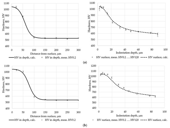
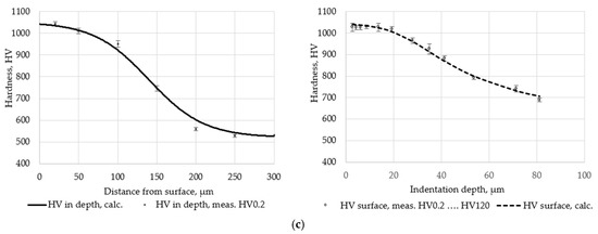
Figure 7.
In-depth hardness (left) and surface hardness calculated from this (right): (a) 60 min nitrocarburizing; (b) 120 min nitrocarburizing; (c) 480 min nitrocarburizing.
Table 5.
The parameters of the sigmoid curve according to Equation (4) for different nitrocarburizing times.
The standard deviation between the calculated and measured data in the diagrams of Figure 7 can be found in Table 6, in line “in-depth → surface” according to Equation (5).
Table 6.
Standard deviation between measured and calculated surface hardness values.
5.2. In-Depth Hardness Distribution Estimated from Surface Hardness
When calculating the Hd in-depth hardness distribution from the Hs surface hardness data with the inverse calculation (Section 3.2), the parameters of Equation (4) were varied between the limits below:
- A1 maximal (surface) hardness: between 1000 and 1100 HV, in steps of 10 HV;
- A2 minimal (basic) hardness: between 500 and 550 HV, in steps of 10 HV;
- x coordinate of the x0 inflexion point: between 30 and 200 μm, in steps of 1 μm;
- dx/x0 ratio: between 4 and 30, in steps of unity.
Each parameter combination or in-depth hardness distribution defines a surface hardness series, which can be determined according to Section 3.1. The parameter combination ensuring the best fit is the combination where the difference (standard deviation) between the measured and calculated data (Equation (5)) is minimal within the parameter range.
Figure 8 shows the results of the inverse calculation for all three nitrocarburizing technologies. The left diagrams show the surface hardness as a function of indentation depth measured with the loads defined in Section 4. These diagrams also show the Hs(h) functions determined according to the above. These Hs(h) functions fit the data series of the surface hardness tests with the lowest error. In the figures on the right, the diagram lines represent the Hd(x) in-depth hardness distribution that belongs to the best surface hardness fitting. The same diagram contains the measured in-depth hardness for each. The surface → in-depth row of Table 6 contains the difference and the standard deviation of measured and calculated results shown in the diagrams of Figure 8. The final result of the inverse calculation, that is, the parameters of the function describing the in-depth hardness distribution calculated from surface hardness, can be found in Table 7.
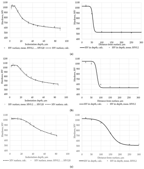
Figure 8.
Surface hardness (left) and the in-depth hardness distribution calculated from this (right): (a) 60 min nitrocarburizing; (b) 120 min nitrocarburizing; (c) 480 min nitrocarburizing.
Table 7.
The parameters of the in-depth hardness distribution function calculated from surface hardness for the three nitrocarburizing variations.
6. Discussion
In general, in the case of surface-treated products, the in-depth hardness distribution can be regarded as the quality parameter of the surface layer. The advantage of the new method presented in this study is that the relationship can be estimated by a non-destructive way, that is, by measuring the surface hardness under different loading conditions.
The core idea of the model is a volumetric approach of the indentation plastic zone (as Ichimura interpreted it [31,32]), which describes the relationship between the Hs(h) surface hardness and the Hd(x) in-depth hardness functions.
In theory, a given in-depth hardness distribution function can be converted into a corresponding surface hardness function, and a surface hardness function can be converted into a corresponding in-depth hardness distribution function.
A comparison of the parameters of the function fitted to the original in-depth hardness data (Table 5) and the function best fitting the surface hardness data (Table 7) indicates that the hardness of the surface (A1) and the basic matrix (A2) can be estimated with adequate accuracy. The location of the inflexion point (x0) can also be appropriately estimated; the maximum of the difference is around 6–7 μm.
The horizontal stretching of the hardness function, the x0/dx parameter, is typically higher in the surface → in-depth conversion (Table 7). This means that from the surface hardness data, a steeper hardness transition is calculated around the inflexion point than what could be concluded from the measured in-depth hardness data. It is clear that one of the factors contributing to the difference is when the hardness of the section perpendicular to the surface is tested, the hardness gradient is also influenced by the size of the indentation, and it is most characteristic around the inflexion point. For example, the HV0.2 indentation diagonal at 700 HV is 23 μm; therefore, there can be a 150–200 HV difference between the two ends of the diagonal in the hardness of the material under the indentation.
7. Conclusions
The mathematical model presented in this paper establishes a direct connection between cross-sectional in-depth hardness distribution and surface hardness data. The following conclusions can be drawn from the model and its adaptation:
- The practical applicability of the presented theoretical model was checked in three case studies (Section 5).
- The standard deviation between the measured and calculated values (Table 6) indicates the possible practical applicability of the model. In the examined cases, the in-depth hardness distribution could be estimated with sufficient accuracy from surface hardness.
- By setting appropriate parameters, the model can be applied to other monolayer cases.
In order to assess the limits of applicability of the presented procedure, a number of issues need further investigation. It should be examined, for example, how the accuracy of the estimation is affected by the well-known uncertainty or measurement error of hardness testing. Moreover, what modifications are necessary to adopt the calculation method for the large variety of surface layers (different types, structures, and thickness and hardness distributions)?
Author Contributions
Writing—original draft preparation, M.R.; conceptualization, M.R.; writing—review and editing, R.H.; investigation, A.S.; methodology, T.R.; validation, T.R., V.G.; formal analysis, V.G.; supervision, I.F. All authors have read and agreed to the published version of the manuscript.
Funding
This research was funded by the 1.3.1-VKE-2017-00025 project.
Institutional Review Board Statement
Not applicable.
Informed Consent Statement
Not applicable.
Data Availability Statement
The data presented in this study are available on request from the corresponding author.
Conflicts of Interest
The authors declare no conflict of interest. The funders had no role in the design of the study; in the collection, analyses, or interpretation of data; in the writing of the manuscript; or in the decision to publish the results.
References
- Westbrook, J.H. The Science of Hardness Testing and Its Research Applications; American Society for Metals: Metals Park, OH, USA, 1973; p. 453. [Google Scholar]
- Burnett, P.J.; Page, T.F. Surface softening in silicon by ion implantation. J. Mater. Sci. 1984, 19, 845–860. [Google Scholar] [CrossRef]
- Jönsson, B.; Hogmark, S. Hardness measurements of thin films. Thin Solid Films 1984, 114, 257–269. [Google Scholar] [CrossRef]
- Burnett, P.; Rickerby, D. The mechanical properties of wear-resistant coatings: I: Modelling of hardness behaviour. Thin Solid Films 1987, 148, 41–50. [Google Scholar] [CrossRef]
- Johnson, K. The correlation of indentation experiments. J. Mech. Phys. Solids 1970, 18, 115–126. [Google Scholar] [CrossRef]
- Marsh, D.M. Plastic flow in glass. Proc. R. Soc. London. Ser. A Math. Phys. Sci. 1964, 279, 420–435. [Google Scholar] [CrossRef]
- Tabor, D. The hardness of solids. Rev. Phys. Technol. 1970, 1, 145–179. [Google Scholar] [CrossRef]
- Tuck, J.; Korsunsky, A.; Davidson, R.; Bull, S.; Elliott, D. Modelling of the hardness of electroplated nickel coatings on copper substrates. Surf. Coat. Technol. 2000, 127, 1–8. [Google Scholar] [CrossRef]
- Tuck, J.R.; Korsunsky, A.M.; Bull, S.J.; Davidson, R.I. On the application of the work-of-indentation approach to depth-sensing indentation experiments in coated systems. Surf. Coat. Technol. 2001, 137, 217–224. [Google Scholar] [CrossRef]
- Puchi-Cabrera, E. A new model for the computation of the composite hardness of coated systems. Surf. Coat. Technol. 2002, 160, 177–186. [Google Scholar] [CrossRef]
- Iost, A.; Guillemot, G.; Rudermann, Y.; Bigerelle, M. A comparison of models for predicting the true hardness of thin films. Thin Solid Films 2012, 524, 229–237. [Google Scholar] [CrossRef]
- Coorevits, T.; Mejias, A.; Montagne, A.; Kossman, S.; Iost, A. An integral approach of indentation of Functionally Graded Materials. Surf. Coat. Technol. 2020, 381, 125176. [Google Scholar] [CrossRef]
- Khalaj, G. Artificial neural network to predict the effects of coating parameters on layer thickness of chromium carbonitride coating on pre-nitrided steels. Neural Comput. Appl. 2013, 23, 779–786. [Google Scholar] [CrossRef]
- Khalaj, G.; Pouraliakbar, H. Computer-aided modeling for predicting layer thickness of a duplex treated ceramic coating on tool steels. Ceram. Int. 2014, 40, 5515–5522. [Google Scholar] [CrossRef]
- Lawn, B.R.; Evans, A.G.; Marshall, D.B. Elastic/Plastic Indentation Damage in Ceramics: The Median/Radial Crack System. J. Am. Ceram. Soc. 1980, 63, 574–581. [Google Scholar] [CrossRef]
- Suresh, S.; Giannakopoulos, A. A new method for estimating residual stresses by instrumented sharp indentation. Acta Mater. 1998, 46, 5755–5767. [Google Scholar] [CrossRef]
- Giannakopoulos, A.; Suresh, S. Determination of elastoplastic properties by instrumented sharp indentation. Scr. Mater. 1999, 40, 1191–1198. [Google Scholar] [CrossRef]
- Nayebi, A.; El Abdi, R.; Bartier, O.; Mauvoisin, G. New procedure to determine steel mechanical parameters from the spherical indentation technique. Mech. Mater. 2002, 34, 243–254. [Google Scholar] [CrossRef]
- Nayebi, A.; El Abdi, R.; Bartier, O.; Mauvoisin, G. Hardness profile analysis of elasto-plastic heat-treated steels with a gradient in yield strength. Mater. Sci. Eng. A 2002, 333, 160–169. [Google Scholar] [CrossRef]
- Chen, J.; Bull, S. On the relationship between plastic zone radius and maximum depth during nanoindentation. Surf. Coat. Technol. 2006, 201, 4289–4293. [Google Scholar] [CrossRef]
- Klecka, M.A.; Subhash, G.; Arakere, N.K. Determination of Subsurface Hardness Gradients in Plastically Graded Materials via Surface Indentation. J. Tribol. 2011, 133, 031403. [Google Scholar] [CrossRef]
- Kuram, E. The effect of monolayer TiCN-, AlTiN-, TiAlN-and two layers TiCN + TiN- and AlTiN + TiN-coated cutting tools on tool wear, cutting force, surface roughness and chip morphology during high-speed milling of Ti6Al4V titanium alloy. Proc. Inst. Mech. Eng. Part B J. Eng. Manuf. 2016, 232, 1273–1286. [Google Scholar] [CrossRef]
- Wang, C.; Wang, X.; Sun, F. Tribological behavior and cutting performance of monolayer, bilayer and multilayer diamond coated milling tools in machining of zirconia ceramics. Surf. Coat. Technol. 2018, 353, 49–57. [Google Scholar] [CrossRef]
- Ahmed, Y.S.; Youssef, H.; El-Hofy, H.; Ahmed, M. Prediction and Optimization of Drilling Parameters in Drilling of AISI 304 and AISI 2205 Steels with PVD Monolayer and Multilayer Coated Drills. J. Manuf. Mater. Process. 2018, 2, 16. [Google Scholar] [CrossRef]
- Al-Tameemi, H.; Al-Dulaimi, T.; Awe, M.; Sharma, S.; Pimenov, D.; Koklu, U.; Giasin, K. Evaluation of Cutting-Tool Coating on the Surface Roughness and Hole Dimensional Tolerances during Drilling of Al6061-T651 Alloy. Materials 2021, 14, 1783. [Google Scholar] [CrossRef]
- Gharbi, A.; Bouhamla, K.; Ghelloudj, O.; Ramoul, C.E.; Berdjane, D.; Chettouh, S.; Remili, S. Heat Treatment Effect on the Microstructural, Hardness and Tribological Behavior of A105 Medium Carbon Steel. Defect Diffus. Forum 2021, 406, 419–429. [Google Scholar] [CrossRef]
- Li, Y.; He, Y.; Xiu, J.; Wang, W.; Zhu, Y.; Hu, B. Wear and corrosion properties of AISI 420 martensitic stainless steel treated by active screen plasma nitriding. Surf. Coat. Technol. 2017, 329, 184–192. [Google Scholar] [CrossRef]
- Biehler, J.; Hoche, H.; Oechsner, M. Nitriding behavior and corrosion properties of AISI 304L and 316L austenitic stainless steel with deformation-induced martensite. Surf. Coat. Technol. 2017, 324, 121–128. [Google Scholar] [CrossRef]
- Adachi, S.; Ueda, N. Wear and Corrosion Properties of Cold-Sprayed AISI 316L Coatings Treated by Combined Plasma Carburizing and Nitriding at Low Temperature. Coatings 2018, 8, 456. [Google Scholar] [CrossRef]
- Mata, M.; Casals, O.; Alcalá, J. The plastic zone size in indentation experiments: The analogy with the expansion of a spherical cavity. Int. J. Solids Struct. 2006, 43, 5994–6013. [Google Scholar] [CrossRef]
- Ichimura, H.; Rodriguez, F.; Rodrigo, A. The composite and film hardness of TiN coatings prepared by cathodic arc evaporation. Surf. Coat. Technol. 2000, 127, 138–143. [Google Scholar] [CrossRef]
- Ichimura, H.; Ishii, Y.; Rodrigo, A. Hardness analysis of duplex coating. Surf. Coat. Technol. 2003, 169-170, 735–738. [Google Scholar] [CrossRef]
Publisher’s Note: MDPI stays neutral with regard to jurisdictional claims in published maps and institutional affiliations. |
© 2021 by the authors. Licensee MDPI, Basel, Switzerland. This article is an open access article distributed under the terms and conditions of the Creative Commons Attribution (CC BY) license (https://creativecommons.org/licenses/by/4.0/).