Dealing with the Fracture Ductile-to-Brittle Transition Zone of Ferritic Steels Containing Notches: On the Applicability of the Master Curve

Abstract

Characterizing the fracture resistance of ferritic steels operating within their Ductile-to-Brittle Transition Zone (DBTZ) has been successfully addressed through the development of the well-known Master Curve (MC). This tool assumes that fracture, in the presence of crack-like defects, is controlled by weakest-link statistics and follows a three-parameter Weibull distribution. When dealing with notch-type defects, there is no standardized solution to predict the fracture resistance within the DBTZ, but the authors have published some works demonstrating that the MC can also be applied in different ways to characterize ferritic steels containing notches. One of these ways is the direct application of the MC methodology, providing a specific reference temperature (T₀^N) for each material and notch radius. This work reviews this initial attempt to apply the MC in notched conditions, assessing the validity of the main MC hypotheses (initially valid for cracked conditions) when analyzing notch-type defects and providing experimental validation on steels S275JR, S355J2, S460M and S690Q.

1. Introduction

The analysis of the ductile-to-brittle transition zone (DBTZ) of ferritic steels has been widely performed over the years. These steels generally have structural functions, and the presence of defects such as cracks or notches (often unavoidable) together with sufficiently low operating temperatures may jeopardize the corresponding structural integrity. In industrial or engineering practice, the main tool used to characterize the material fracture toughness within the DBTZ is the master curve (MC) (e.g., [1,2,3,4,5]), which, based on weakest-link statistics and assuming a three-parameter Weibull distribution, defines the whole DBTZ through the material reference temperature, T₀.

The MC has been derived and defined to be applied in cracked conditions; however, the defects found in ferritic steels may have a certain finite radius on their tip. These defects are generally referred to as notches and have also been the subject of abundant research in the last few decades [6]. Notches generate less demanding stress fields than cracks, and this may be coupled with changes in fracture micromechanisms [7,8]. As a result, the apparent fracture toughness of ferritic steels containing notches can be much higher than the fracture toughness developed in cracked conditions, and the corresponding load-bearing capacity of the structural components may also be considerably larger. The sensitivity of a particular material to this notch effect is not evident beforehand, with materials developing intense notch effects from very small notch radii (e.g., [9,10]), and materials with negligible notch effects (i.e., notches behaving like cracks) even for significant notch radii (e.g., [11,12]). In any case, assuming that the fracture behavior of ferritic steels containing notches and operating within the DBTZ is the same as that developed in cracked conditions is generally an over-conservative practice, and a specific tool is required for a better definition of a material’s fracture behavior under such circumstances.

In this sense, the authors have previously published some literature with a view to addressing this issue [13,14,15], with two main alternatives. The first one (referred to as the notch master curve, NMC) consists of defining T₀ for cracked conditions and applying a subsequent notch correction through (for example) the Theory of Critical Distances (TCD). The second one consists of the direct application of the MC to the notched material, deriving the corresponding notch (or apparent) Reference Temperature (T₀^N), which depends on the material being analyzed and the notch radius being considered. This second option does not require any additional notch correction.

This paper is focused on the second methodology (the reasons being explained below), providing a review of the different hypotheses that are implicitly being assumed and analyzing their validity, and including additional validation supporting the use of the MC in the characterization of the DBTZ of ferritic steels containing notches. The empirical nature of the approach makes it necessary to limit its validity to the materials covered here. Any generalized use, with predictive purposes, would require a much more extensive validation program.

In summary, Section 2 provides an overview of the MC, and Section 3 gathers a description of the two methodologies developed by the authors to analyze the DBTZ of ferritic steels, with particular emphasis on the direct application of the MC. Section 4 provides insights and discussion about the hypotheses sustaining this practice, together with the provision of experimental validation by using fracture results on steels S275JR, S355J2, S460M and S690Q. Finally, Section 5 presents the main conclusions.

2. The Master Curve: Brief Overview

The master curve (MC) [1,2,3,4,5] is a fracture characterization methodology for ferritic steels containing crack-like defects and working within their ductile-to-brittle transition zone (DBTZ). The MC is based on statistical assumptions associated with the distribution of cleavage-promoting particles around the crack tip and considers that cleavage fracture is triggered by the existence of such particles. Consequently, fracture is essentially an initiation-dependent process that is presumed to be dominated by weakest-link statistics and follows a three-parameter Weibull distribution. As a result, and within the scope of small-scale yielding conditions, the cumulative failure probability (P_f) on which the MC is based follows Equation (1):

P_f = 1 − e^{(B/B₀)·{(K_Jc − K_min)/(K₀ − K_min)}b}

(1)

where K_Jc is the fracture toughness for a given probability of failure (P_f), B is the component thickness, B₀ is the reference thickness, and K₀ is the Weibull scale parameter located at the 63.2% cumulative probability of failure. K_min and b are the other two parameters of the Weibull distribution and, based on experimental fittings, they are assumed to take constant values for all ferritic steels: K_min (location parameter) is fixed at 20 MPam^1/2 and b (shape parameter) is set equal to 4, respectively [1,2,3,4]. The fracture characterization is thus performed by using K_Jc, an elastic–plastic equivalent stress intensity factor derived from the J-integral at the onset of cleavage fracture, J_c.

Under cleavage fracture conditions, K₀ depends on the temperature following Equation (2) [1,2,3,4]:

K₀ = 31 + 77e^{0.019·(T − T₀)}

(2)

where T is the working temperature and T₀ is the reference temperature, a material property defined as the temperature where the mean (median) fracture toughness for a 25 mm thick (1T) specimen is 100 MPam^1/2. This equation was experimentally fitted from a wide database of fracture toughness results obtained in reactor pressure vessel steels and weldments [16], although, in the case of the 0.019 factor, it has been found that it may actually have some dependence on the material yield strength (σ_ys) and T₀ [17]. Therefore, and provided that K_min and b are considered to be fixed at certain values (20 MPam^1/2 and 4, respectively), the only parameter required to define the temperature dependence of K_Jc is T₀. For any ferritic steel (with a yield strength ranging from 275 to 825 MPa [5]), combining Equations (1) and (2), and assuming the fixed values of b and K_min, it is possible to express the MC for a given probability of failure (P_f):

K_Jc,Pf = 20 + (−ln(1 − P_f))^0.25(11 + 77e^{0.019·(T − T}₀⁾)

(3)

As an example, the curves associated with probabilities of failure of 95, 50 and 5% are provided in Equations (4)–(6), respectively:

K_Jc,0.95 = 34.5 + 101.3e^{0.019·(T − T₀)}

(4)

K_Jc,0.50 = 30.0 + 70.0e^{0.019·(T − T₀)}

(5)

K_Jc,0.05 = 25.2 + 36.6e^{0.019·(T − T₀)}

(6)

The procedure that allows T₀ to be determined has been standardized since 1997 [18], and it is widely accepted in industry. The latest version is ASTM E1921-20 [5]. Details on how T₀ is calculated from fracture toughness test results obtained in cracked specimens may be found in this standard and are not a subject of discussion here.

Equation (3) (as well as Equations (4)–(6)) also assumes that the fracture toughness is being estimated for a thickness equal to that used in the determination of T₀ (i.e., B = B₀).

In the case of ASTM E1921, the reference thickness is 25 mm (B₀ = 25 mm, also referred to as 1T). Furthermore, when the thickness of the component being analyzed is not 25 mm (1T), the authors of [5] provide Equation (7) to derive the fracture toughness value for a given thickness (B_x) from the fracture toughness value for a 25-mm-thick specimen (which follows Equation (3)):

K_Jc(x) = 20 + (K_Jc(0) − 20)(B₀/B_x)^0.25

(7)

where K_Jc(x) is the fracture toughness for a component size B_x, and K_Jc(0) is the fracture toughness for the reference thickness (B₀ = 1 T = 25 mm).

Here, it should be noted that the MC addresses the main issues related to the fracture behavior of ferritic steels within their DBTZ: the temperature dependence of the fracture toughness (see Equation (3)), the specimen thickness dependence (Equation (7)), and the great scatter observed in the experimental results (Equations (3)–(6)).

The standardized procedure [5] also provides a censoring methodology ensuring that the data used in the estimation of T₀ are within the scope of the MC, fulfilling the different hypotheses sustaining this methodology (e.g., high constraint, small-scale yielding, cleavage fracture). More precisely, the remaining specimen ligament, b₀, must have a sufficient size to maintain a condition of high crack-front constraint at fracture and small-scale yielding conditions. This is accomplished by censoring all K_Jc data exceeding the limit established by Equation (8):

K_Jc,limit = {(Eb₀σ_ys)/(30(1 − υ²))}^0.5

(8)

b₀ being the initial ligament length, σ_ys being the material yield strength at the testing temperature, E being the material elastic modulus and υ being the Poisson’s ratio. Another limit, K_JcΔa, is established to censor tests that finish in cleavage after a slow stable crack growth that exceeds a certain limit: the smaller of either 0.05 (W − a₀) or 1 mm, with W being the specimen width and a₀ being the initial crack length. As explained in [5], the resulting censored data are used in the evaluation of T₀, as they contain valuable information: K_Jc data exceeding K_Jc,limit are replaced by K_Jc,limit, whereas if K_JcΔa is violated, data shall be replaced with K_JcΔa. Those data exceeding K_Jc,limit and K_JcΔa shall be replaced by the lower value of the two. For all data, the censoring parameter δ_i is 1 for uncensored and 0 for censored data [4,5]. Finally, any test finished without cleavage fracture, and with a fracture toughness value not exceeding any of the two mentioned limits, will be discarded.

Finally, it is worth mentioning that there have been other attempts to characterize the fracture behavior of ferritic steels within the DBTZ. For example, refined models may be found in [19,20,21,22], generally based on the statistical nature of K_Jc, providing important insights into the phenomenon being studied, but with significant difficulties for their industrial practice. Other proposals attempt to develop a simpler application but provide less mechanistic understanding [23].

3. The Ductile-to-Brittle Transition Zone in Notched Conditions

The MC methodology described above assumes that the defect causing the (cleavage) fracture process is a crack (i.e., a sharp defect with parallel faces and a radius on the tip that tends to zero). However, in industrial practice, the defects that may cause the failure of a particular structural component are not necessarily crack-like defects and may have a finite radius on their tip. Such defects are here referred to as notches. In such cases, the stress field becomes more relaxed, the material may develop a higher fracture resistance (usually referred to as the apparent fracture toughness) and, consequently, the load-bearing capacity of the corresponding structural component may also be larger. The concept of apparent fracture toughness has important implications: experimentally, it is obtained in notched specimens, generating the corresponding load–displacement curves, and subsequently obviating that the defect is actually a notch, applying the corresponding standard formulation (e.g., [24]) proposed for cracked specimens. In other words, the real notched situation is assumed to be a cracked situation on which the material develops higher fracture resistance (the apparent fracture toughness).

The scientific literature provides a number of documents and substantial evidence revealing how the introduction of a finite radius on the defect tip causes a significant increase in the fracture resistance of different materials (e.g., [6,7,8,9,10,25,26,27,28,29,30,31,32,33,34]). Thus, it is necessary to define methodologies to assess components containing notches. The case of ferritic steels operating within the DBTZ constitutes a particular case in which the fracture toughness in cracked conditions may be analyzed within a significant range of temperatures by using one single tool, the MC. In the case of ferritic steels containing notches, it would be of great interest to have an analogous tool defining the apparent fracture toughness throughout the corresponding DBTZ.

The first obvious option is to treat notches as if they were cracks, considering that the DBTZ is the same for cracks and notches. If applying the MC, this implies using the same reference temperature (T₀) for cracks and notches, as well as the same equations (Equations (3)–(6)). T₀ would be obtained in cracked specimens and subsequently applied to both cracks and notches regardless of the notch radius. Obviously, this is generally an overconservative practice, and it is not an acceptable approach from both the scientific and engineering points of view.

To the knowledge of the authors, the different models dealing with the notch effect within the DBTZ are those proposed by Schindler et al. [35], Cicero et al. [13,14] and García and Cicero [15].

Schindler et al. [35] combine the MC with an expression to account for the notch effect (i.e., notch effect correction) in the apparent fracture toughness expression. They conclude that the shape of the transition curve is affected by the notch radius, which generates a bump on the median curve. The magnitude of this bump depends on the notch radius and on material properties but, in any case, impedes using the MC methodology prescribed by ASTM E1921 [5]. Thus, when applying the MC methodology, T₀ has to be estimated from tests performed on sharply notched specimens, either by an adjusted reference level of K_ref^N (instead of 100 MPa·m^0.5) or by a shift in the apparent reference temperature T₀^N. Another interesting point of this research is that it also found that the 0.019 coefficient included in the different MC equations may be a reasonable value when analyzing notches. The reader is referred to the original source [35] for further details.

Cicero et al. [13,14] proposed the use of the notch master curve. This methodology consists of defining the MC (and T₀) from cracked specimens, as per ASTM E1921 [5], and multiplying the corresponding equation by a notch correction factor. More precisely, the authors proposed the use of the notch correction derived from the combination of the Line Method (Theory of Critical Distances, TCD) [6] and the Creager–Paris stress distribution [36] ahead of a notch tip.

K_Jc,Pf = {20 + (−ln(1 − P_f))^0.25(11 + 77e0.019 (T − T₀))}·(1 + (0.25 ρ/L))^0.5

(9)

The notch correction depends on the notch radius (ρ) being analyzed and the material critical distance (L), which was shown to vary with temperature within the DBTZ [13,14]. In spite of such variation, it was also shown that using an average value of L for the whole DBTZ generated good predictions of the apparent fracture toughness within the temperature range of T₀ ± 50 °C, which is the validity range of the MC itself. From the mathematical expression shown in Equation (9), it is straightforward to verify that the shape of the NMC differs from the shape of the MC.

In any case, the NMC only applies one of the notch corrections provided by the TCD to the fracture toughness obtained in cracked conditions, with the particularity of using the MC for the estimation of the fracture toughness. Given that the validity of the MC (e.g., [1,2,3,4,16,17]) and the TCD corrections (e.g., [6,7,8,9,10,11,12,13,14,15]) is widely reported in the literature, there are no major theoretical issues when applying this methodology. Its main difficulty is the amount of experimental work required for a complete description of the NMC, as this requires defining not only T₀, but also the values of L throughout the DBTZ. Effectively, and as well as having to obtain T₀, the definition of L requires testing cracked and notched specimens with different notch radii. Moreover, because of the inherent scatter of fracture results within the DBTZ, several tests must be completed per notch radius. Thus, the combination of different temperatures, notch radii and test repetitions requires significant experimental work (see [6,7,8,9,10,11,12,13] for details about the calibration process of L).

With all this, from this point, this work will be focused on the direct application of the MC by testing specimens with the notch radius of interest, following the experimental procedure and the formulation included in ASTM 1921 [5]. The resulting parameter will not be T₀ (as is the case in cracked specimens), but a new parameter referred to as the notch (or apparent) reference temperature (T₀^N). Finally, T₀^N is included in the MC formulation substituting T₀. The resulting equations are:

K^N_Jc,Pf = 20 + (−ln(1 − P_f))^0.25(11 + 77e^{0.019·(T − T₀N)})

(10)

K^N_Jc,0.95 = 34.5 + 101.3e^{0.019·(T − T₀N)}

(11)

K^N_Jc,0.50 = 30.0 + 70.0e^{0.019·(T − T₀N)}

(12)

K^N_Jc,0.05 = 25.2 + 36.6e^{0.019·(T − T₀N)}

(13)

K^N_Jc being the apparent fracture toughness for the notch radius analyzed. Equations (11)–(13) are associated with probabilities of failure of 95, 50 and 5%, respectively. This formulation was applied in [15] to steels S275JR and S355J2, providing satisfactory predictions of the apparent fracture toughness within the range T₀^N ± 50 °C. However, in order to generally apply the MC to notched ferritic steels, it is necessary to justify that the different hypotheses sustaining the MC in cracked conditions are also valid when analyzing notches (this was not done in [15]), and also to validate the methodology by using a wider experimental program. These two needs are addressed in Section 4.

Finally, alternative approaches to analyze the notch effect within the DBTZ could be derived from other well-established theories, such as the SED criterion [25,26,27,28,29] or notch fracture mechanics [37,38].

4. On the Applicability of the MC in Notched Conditions: Hypotheses and Validation

As mentioned above, the application of the MC in notched conditions requires justifying that the different hypotheses sustaining the use of the MC when analyzing ferritic steels containing crack-like defects are also valid when the defects being analyzed are notches. These hypotheses are gathered and discussed below, with the corresponding justification of their use in notched conditions. The experimental values used in this section are gathered in Appendix A, which comprises previous fracture tests developed by the authors on cracked and notched specimens made of steels S275JR [13,15], S355J2 [13,15], S460M [14] and S690Q [14]. Appendix A also shows the resulting reference temperatures (T₀) or apparent reference temperatures (T₀^N) per combination of material and defect radius. These temperatures are obtained by directly applying the MC methodology [5], regardless of the type of defect (crack or notch) being analyzed and following multi-temperature formulation [5].

The different hypotheses sustaining the MC in cracked conditions, and the discussion about their applicability to notched conditions, are the following:

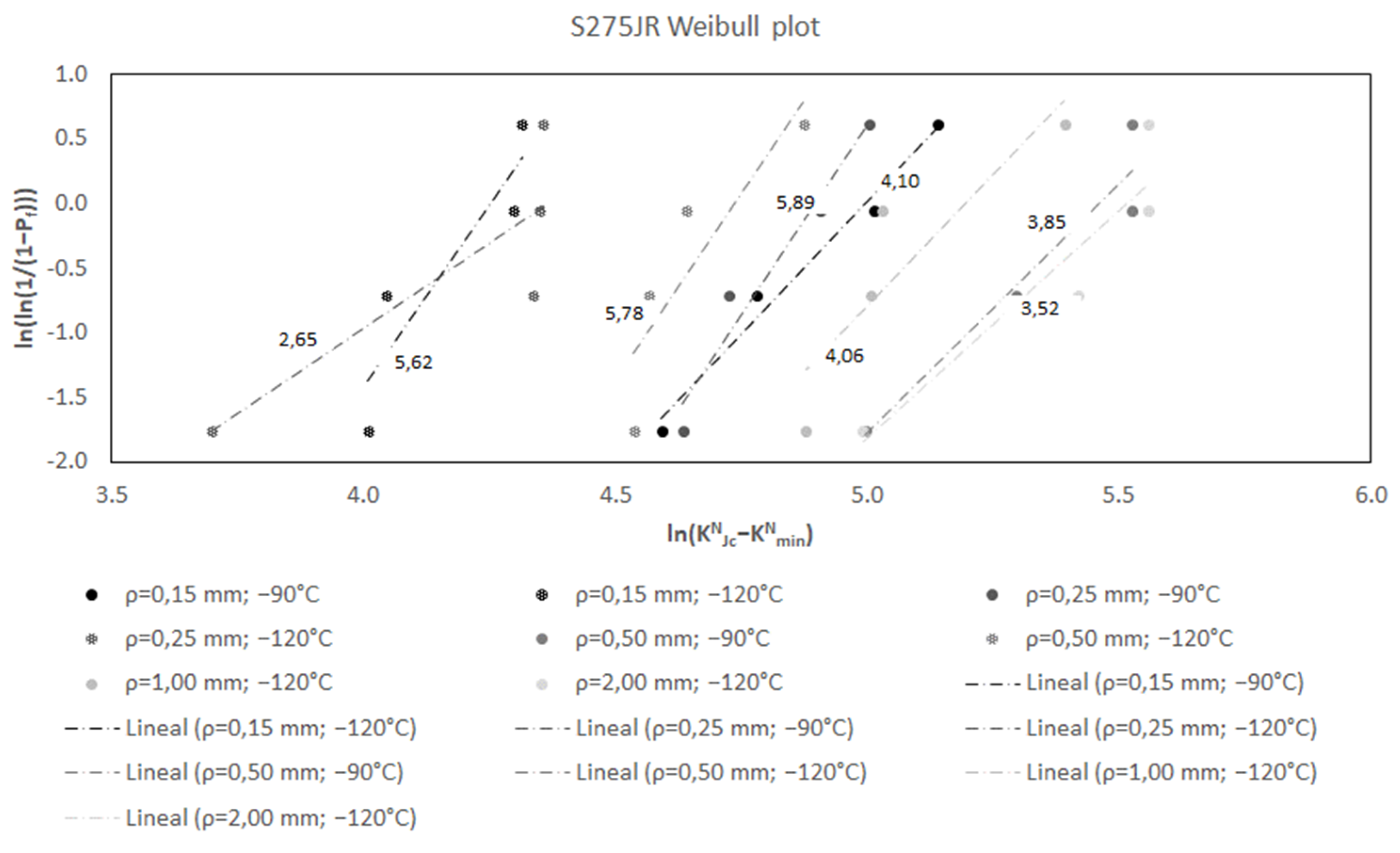
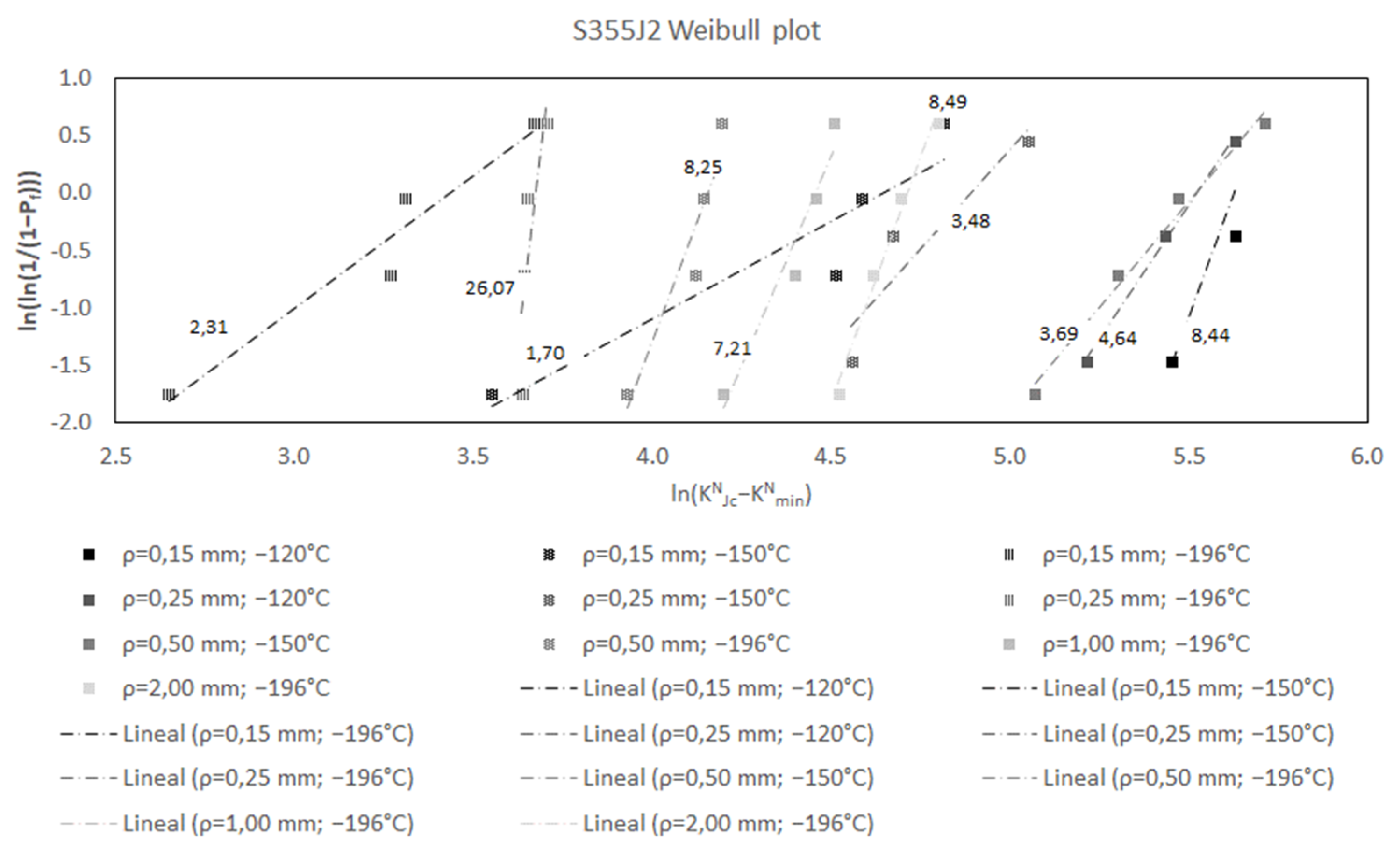
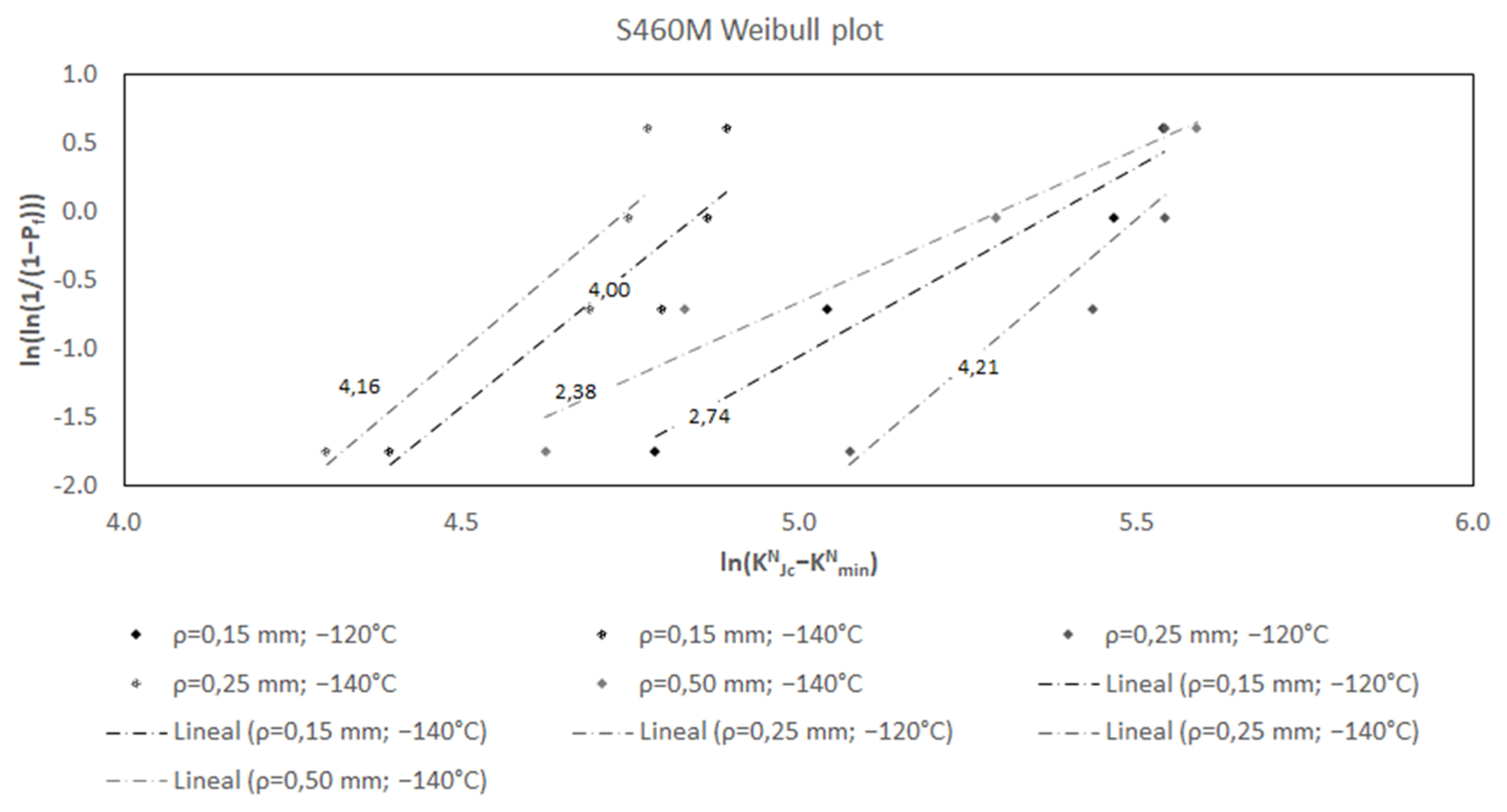
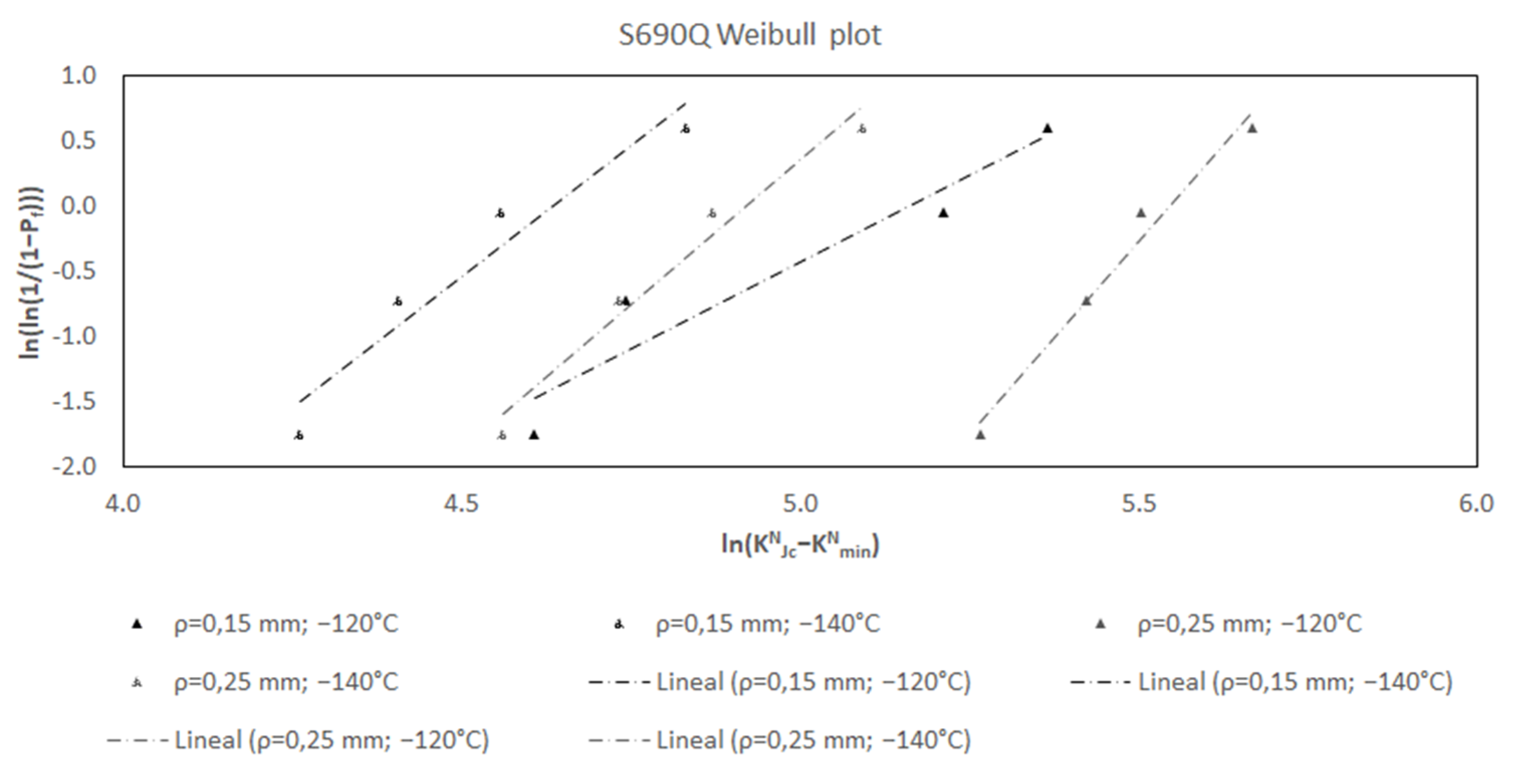
• Weibull distribution: when dealing with notch-type defects in ferritic steels within the corresponding DBTZ, the failure mechanism is also cleavage, and as it is assumed in cracked situations, the fracture process obeys weakest-link statistics. This kind of phenomenon, also presenting a minimum value of the fracture toughness below which there is no cleavage fracture, is conveniently described by a (three-parameter) Weibull distribution. In other words, given that the fracture processes in cracked and notched conditions, at their respective DBTZs, have the same fracture micromechanisms, an analogous Weibull distribution should also be suitable for the analysis of notches. The cumulative failure probability (P_f) follows Equation (14):

  P_f = 1 − e^{(B/B₀)·{(KN_Jc − KN_min)/(KN₀ − KN_min)}bN}

  (14)
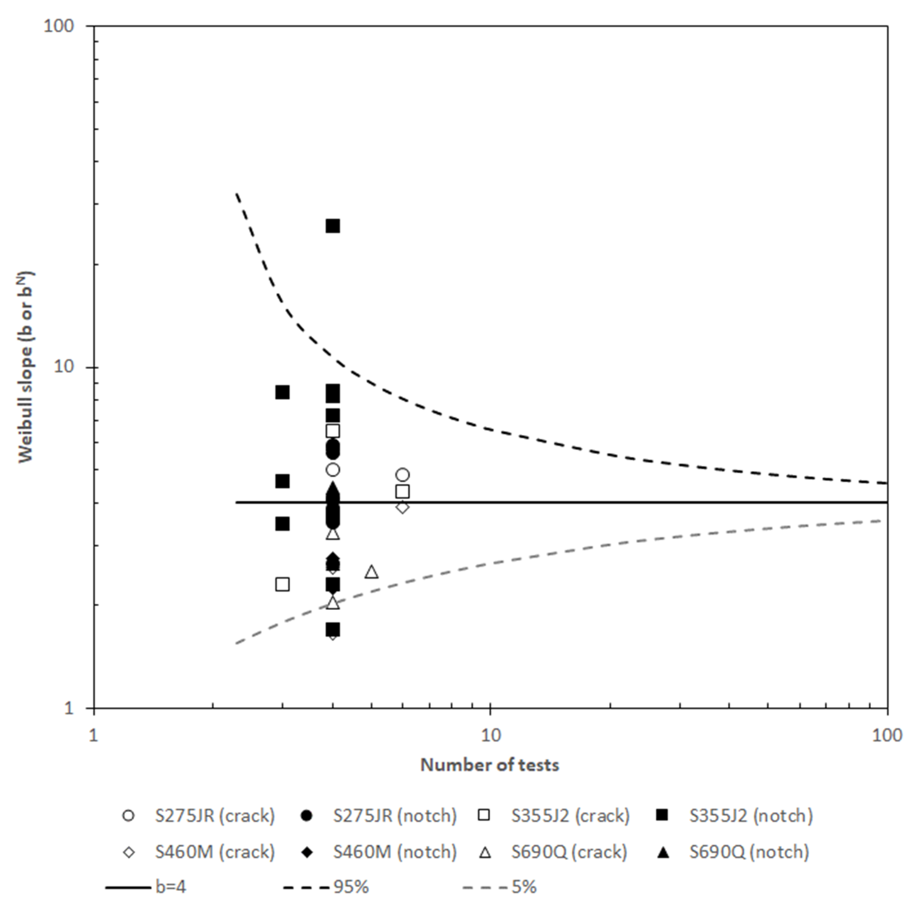
• b^N: the shape parameter of the Weibull distribution (Weibull slope) is assumed to be 4 in the MC, and statistical analyses [4] confirm that this value is adequate in cracked conditions. Following the same reasoning, Figure 1, Figure 2, Figure 3, Figure 4, show the different b^N values (slopes) obtained in a number of datasets developed by the authors (the complete list of experimental results is gathered in Appendix A), for different materials and notch radii (results in cracked conditions are also included). In the figures, K^N_min has been assumed to be equal to 20 MPam^1/2 (see discussion below). Each dataset includes at least three K^N_Jc values satisfying ASTM E1921 validity requirements [5] measured at a single temperature and a single loading rate using a single specimen size with a single notch radius. The K^N_Jc values are then rank ordered and assigned an estimate of the median rank probability (P_f) [39], which is given by:

  P_f = (i − 0.3)/(n + 0.4)

  (15)

  where i is the order of the K^N_Jc value and n is the total number of K^N_Jc values.

Figure 5 shows how the resulting values of b^N fit within the corresponding confidence bands (90% limits) used in the literature (e.g., [39,40]) to justify the value of b = 4 for cracked conditions. It can be observed how the values of b^N (bold symbols) fit well within the confidence bands (25 points out of 27), so it appears reasonable to use this value for notched conditions (b^N = b = 4). Figure 5 also includes the results obtained here in cracked conditions (open symbols) for the tests gathered in Appendix A, which also fit well (as expected) within the confidence bands (11 points out of 12).

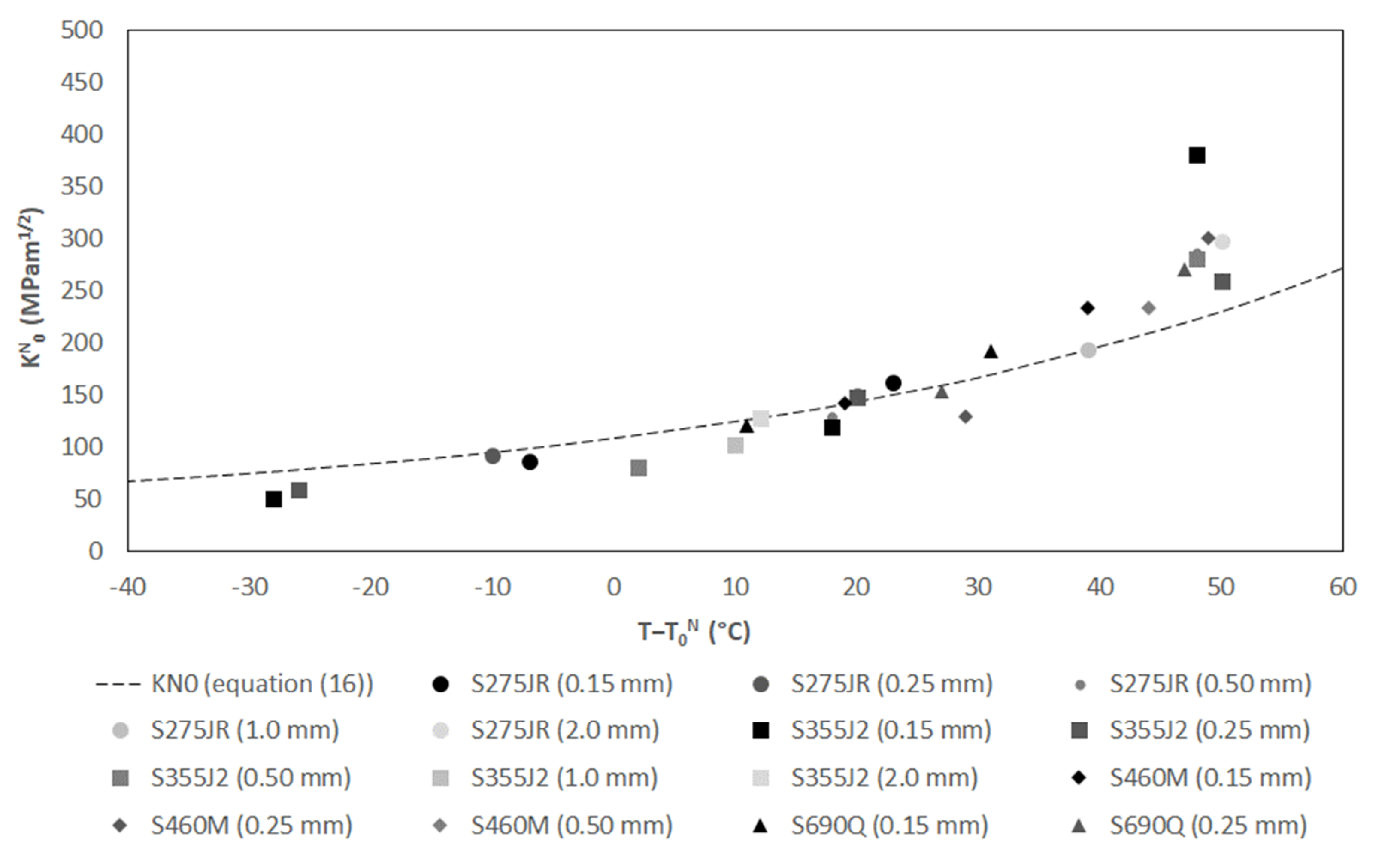
• K^N₀: the scale parameter of the Weibull distribution is the apparent fracture toughness corresponding to a failure probability of 63.2%. The definition of K₀ in cracked conditions (i.e., its temperature dependence) was empirically fitted from a wide set of experimental results [16], where it was shown that regardless of the ferritic steel and the irradiation damage, all K₀ − T tests had the same shape. The fitting curve is shown in Equation (2) [16], which, in Figure 6, is represented in terms of K^N₀ − (T − T₀^N) for the different test results and datasets gathered in Appendix A. Each dataset (i.e., each point of the curve) corresponds to a combination of material, temperature and notch radius, with K^N₀ being obtained by using the maximum likelihood method [5]:

  K^N₀ = [Σⁿ_{i = 1} (K^N_Jc,i − 20)⁴/r]^0.25 + 20

  (16)

  where n is the total number of data (censored and uncensored), and r is the number of uncensored data. Again, Equation (16) assumes that K^N_min is equal to 20 MPam^1/2 (see discussion below). The results shown in Figure 6 suggest that K^N₀ may be slightly underestimated for T − T₀^N values between 0 and −50 °C, and also that it could be overestimated for T − T₀^N values close to +50 °C. In any case, it can be observed that the datasets of notched specimens follow reasonably well the fitting equation. Thus, analogously to Equation (2) in cracked conditions, it appears reasonable to use Equation (17) for notched conditions:

  K^N₀ = 31 + 77e^{0.019·(T − T}₀^N)

  (17)
• K^N_min: the location parameter of the Weibull distribution is also necessary in notched conditions, as cleavage requires a minimum stress intensity factor to occur. Thus, a three-parameter Weibull distribution is also required when analyzing notches (with K^N_min being the third parameter). Concerning the value of K^N_min, it is proposed to use the same one used for cracks, which is K_min = 20 MPam^1/2. Here, one could argue that in notched conditions, the apparent fracture toughness observed in notched conditions should be higher than 20 MPam^1/2 when this precise value is observed in cracked conditions. This is true, if both fracture toughness and apparent fracture toughness are compared at a given temperature, but it is necessary to consider that K^N_min would not be achieved at the same temperature as K_min, given that the curve obtained in notched conditions is shifted to lower temperatures. Therefore, the hypothesis of considering 20 MPam^1/2 as the minimum value below which cleavage is impossible is also reasonable in notched conditions, even more so if it is considered (again) that in both situations (cracked and notched), fracture is caused by the same micromechanisms. Finally, in any case, considering 20 MPam^1/2 as K^N_min in notched conditions could be argued to be a conservative assumption, whose consequences in the final apparent fracture toughness predictions will be shown below.
• K^N_Jc,limit: the censoring criterion in cracked conditions is established by Equation (8), which is applied to meet small-scale yielding conditions and, thus, to guarantee that the stress fields at fracture are not influenced by the finite size of the fracture specimens being used [39]. Equation (8) is based on different works [41,42] which, based on FE modeling, derived an expression ensuring that the crack-tip stress fields in a finite size specimen do not deviate significantly from the crack-tip stress fields characteristic of an infinite body [39]. A given K_Jc,limit corresponds to a given applied external load and certain size of the plastic zone. K^N_Jc,limit follows the same equations as K_Jc,limit (here, it is important to remember the concept of apparent fracture toughness), so the same values of K_Jc,limit and K^N_Jc,limit correspond to basically the same applied external load. However, physically, when applying the same load to a cracked and a notched specimen, the latter develops a smaller plastic zone. In other words, if Equation (8) guarantees small-scale yielding conditions in cracked conditions, such conditions are surely met in notched conditions. Thus, here, it is proposed to use the same censoring criterion for notches as that used for cracks:

  K^N_Jc,limit = {(Eb₀σ_ys)/(30(1 − υ²))}^0.5

  (18)

This censoring criterion is more severe and conservative when applied to notches. The definition of a notch-specific expression, following analogous reasoning as that gathered in [41,42], is not covered in this work and may be a matter for future research. The results shown below will reveal the degree of conservatism derived from Equation (1).

Once the different hypotheses have been justified, it is concluded that the MC methodology should be applicable to notched conditions, with this application providing the values of apparent reference temperatures (T₀^N) gathered in Appendix A and represented in Figure 7. It can be observed that the main part of the notch effect takes place when changing from cracked conditions to the immediate notch radius (ρ = 0.15 mm), after which the evolution of T₀^N becomes progressively less pronounced.

The validation of this statement is shown in Figure 8, where fracture results in notched specimens made of four different steels [13,14,15] are represented in a K^N_Jc − (T − T₀^N) diagram. It can be observed that the direct application of the MC on notched structural steels, now theoretically justified, provides good estimations of the apparent fracture toughness experimental results within the MC validity range (which, in this case, would be T₀^N ± 50 °C). Considering these results, the above-mentioned possible conservatism associated with the use of K^N_min and K^N_Jc,lim values equal to K_min and K_Jc,lim, respectively, does not seem to be significant. In total, 94 out of 105 experimental results lie within the 5 and 95% probability of failure curves, with three estimations being unsafe (the apparent fracture toughness prediction is larger than the corresponding experimental result), and eight estimations are above the 95% probability of failure curve (i.e., conservative results). Overall, 7 out of 8 of these estimations above the 95% curve correspond to censored results (Figure 8 includes both uncensored and censored results, the latter being shown in Appendix A).

5. Conclusions

This paper provides a review and some insights into the analysis of the apparent fracture toughness in ferritic steels operating within the Ductile-to-Brittle Transition Zone (DBTZ) and containing notches, focusing the study on the applicability of the Master Curve (MC) in notched conditions. The MC is a well-known, standardized methodology for the estimation of the fracture toughness of ferritic steels containing crack-like defects and operating within the DBTZ.

The reasoning of the research is twofold. Firstly, the different hypotheses sustaining the use of the MC in cracked conditions are analyzed, and their corresponding use in notched conditions is subsequently demonstrated or justified. Then, a number of experimental results in four different structural steels (S275JR, S355J2, S460M and S690Q) containing different notch radii (ranging from 0.15 to 2.0 mm) are compared with the resulting predictions of the MC. The results show that the application of the MC in notched conditions, now theoretically justified, provides good estimations of the apparent fracture toughness within the DBTZ of the four mentioned materials. Additional validation, in a wider range of structural steels, is required for generalized use of the approach.

References

1. Wallin, K. The scatter in KIc results. Eng. Fract. Mech. 1984, 19, 1085–1093. [Google Scholar] [CrossRef]
2. Wallin, K.; Saario, T.; Törrönen, K. Statistical model for carbide induced brittle fracture in steel. Metal Sci. 1984, 18, 13–16. [Google Scholar] [CrossRef]
3. Wallin, K. The size effect in KIC results. Eng. Fract. Mech. 1985, 22, 149–163. [Google Scholar] [CrossRef]
4. Wallin, K. Master Curve Analysis of Ductile to Brittle Transition Region Fracture Toughness Round Robin Data. The ‘‘EURO’’ Fracture Toughness Curve; VTT Publications 367; Julkaisija-Utgivare Publisher: Helsinki, Finland, 1998. [Google Scholar]
5. ASTM 1921-20. Standard Test Method for the Determination of Reference Temperature, T0, for Ferritic Steels in the Transition Range; American Society for Testing and Materials: Philadelphia, PA, USA, 2020. [Google Scholar]
6. Taylor, D. The Theory of Critical Distances: A New Perspective in Fracture Mechanics; Elsevier: Amsterdam, The Netherlands, 2007. [Google Scholar]
7. Cicero, S.; Madrazo, V.; García, T.; Cuervo, J.; Ruiz, E. On the notch effect in load bearing capacity, apparent fracture toughness and fracture mechanisms of polymer PMMA, aluminium alloy Al7075-T651 and structural steels S275JR and S355J2. Eng. Fail. Anal. 2013, 29, 108–121. [Google Scholar] [CrossRef]
8. Cicero, S.; Madrazo, V.; García, T. Analysis of notch effect in the apparent fracture toughness and the fracture micromechanisms of ferritic–pearlitic steels operating within their lower shelf. Eng. Fail. Anal. 2014, 36, 322–342. [Google Scholar] [CrossRef] [Green Version]
9. Cicero, S.; Madrazo, V.; Carrascal, I.A. Analysis of notch effect in PMMA by using the Theory of Critical Distances. Eng. Fract. Mech. 2012, 86, 56–72. [Google Scholar] [CrossRef]
10. Madrazo, V.; Cicero, S.; Carrascal, I.A. On the point method and the line method notch effect predictions in Al7075-T651. Eng. Fract. Mech. 2012, 79, 363–379. [Google Scholar] [CrossRef]
11. Cicero, S.; García, T.; Castro, J.; Madrazo, V.; Andrés, D. Analysis of notch effect on the fracture behaviour of granite and lime-stone: An approach from the Theory of Critical Distances. Eng. Geol. 2014, 177, 1–9. [Google Scholar] [CrossRef] [Green Version]
12. Justo, J.; Castro, J.; Cicero, S. Notch effect and fracture load pre-dictions of rock beams at different temperatures using the theory of critical distances. Int. J. Rock Mech. Min. Sci. 2020, 125, 104161. [Google Scholar] [CrossRef]
13. Cicero, S.; Madrazo, V.; García, T. The Notch Master Curve: A proposal of Master Curve for ferritic-pearlitic steels in notched conditions. Eng. Fail. Anal. 2014, 42, 178–196. [Google Scholar] [CrossRef] [Green Version]
14. Cicero, S.; García, T.; Madrazo, V. Application and validation of the notch master curve in medium and high strength structural steels. J. Mech. Sci. Technol. 2015, 29, 4129–4142. [Google Scholar] [CrossRef] [Green Version]
15. García, T.; Cicero, S. Application of the Master Curve to ferritic steels in notched conditions. Eng. Fail. Anal. 2015, 58, 149–164. [Google Scholar] [CrossRef]
16. Wallin, K. Irradiation damage effects on the fracture toughness transition curve shape for reactor pressure vessel steels. Int. J. Press Vessel. Pip. 1993, 55, 61–79. [Google Scholar] [CrossRef]
17. Wallin, K. Application of Master Curve to Highly Irradiated RPV Steels. In Proceedings of the LONGLIFE Final International Workshop: RPV steel embrittlement under long term operation conditions, Dresden, Germany, 15–16 January 2014. [Google Scholar]
18. ASTM 1921-97. Standard Test Method for the Determination of Reference Temperature, T0, for Ferritic Steels in the Transition Range; American Society for Testing and Materials: Philadelphia, PA, USA, 1997. [Google Scholar]
19. Beremin, F.M.; Pineau, A.; Mudry, F.; Devaux, J.C.; D’Escatha, Y.; Ledermann, P. A local criterion for cleavage fracture of a nuclear pressure vessel steel. Metall. Mater. Trans. A 1983, 14, 2277–2287. [Google Scholar] [CrossRef]
20. Mudry, F. A local approach to cleavage fracture. Nucl. Eng. Des. 1987, 105, 65–76. [Google Scholar] [CrossRef]
21. Pineau, A. Development of the local approach to fracture over the past 25 years: Theory and applications. Int. J. Fract. 2006, 138, 139–166. [Google Scholar] [CrossRef]
22. Ruggieri, C.; Dodds, R.H., Jr. An engineering methodology for constraint corrections of elastic–plastic fracture toughness—Part I: A review on probabilistic models and exploration of plastic strain effects. Eng. Fract. Mech. 2015, 134, 368–390. [Google Scholar] [CrossRef]
23. Meshii, T. Characterization of fracture toughness based on yield stress and successful application to construct a lower-bound fracture toughness master curve. Eng. Fail. Anal. 2020, 116, 104713. [Google Scholar] [CrossRef]
24. ASTM 1820-20b. Standard Test Method for Measurement of Fracture Toughness; American Society for Testing and Materials: Philadelphia, PA, USA, 2020. [Google Scholar]
25. Lazzarin, P.; Campagnolo, A.; Berto, F. A comparison among some recent energy-and stress-based criteria for the fracture assessment of sharp V-notched components under Mode I loading. Theor. Appl. Fract. Mech. 2014, 71, 21–30. [Google Scholar] [CrossRef]
26. Campagnolo, A.; Berto, F.; Leguillon, D. Fracture assessment of sharp V-notched components under Mode II loading: A comparison among some recent criteria. Theor. Appl. Fract. Mech. 2016, 85, 217–226. [Google Scholar] [CrossRef]
27. Berto, F.; Lazzarin, P. A review of the volume-based strain energy density approach applied to V-notches and welded structures. Theor. Appl. Fract. Mech. 2009, 52, 183–194. [Google Scholar] [CrossRef]
28. Berto, F.; Lazzarin, P. Recent developments in brittle and quasi-brittle failure assessment of engineeringmaterials by means of local approaches. Mater. Sci. Eng. R 2014, 75, 1–48. [Google Scholar] [CrossRef]
29. Lazzarin, P.; Berto, F. Some expressions for the strain energy in a finite volume surrounding the root of blunt V-notches. Int. J. Fract. 2005, 135, 161–185. [Google Scholar] [CrossRef]
30. Niu, L.S.; Chehimi, C.; Pluvinage, G. Stress field near a large blunted V notch and application of the concept of notch stress intensity factor to the fracture of very brittle materials. Eng. Fract. Mech. 1994, 49, 325–335. [Google Scholar]
31. Pluvinage, G. Fatigue and fracture emanating from notch; the use of the notch stress intensity factor. Nucl. Eng. Des. 1998, 185, 173–184. [Google Scholar] [CrossRef]
32. Torabi, A.R.; Berto, F.; Campagono, A. Elastic-plastic fracture analysis of notched Al 7075-T6 plates by means of the local energy combined with the equivalent material concept. Phys. Mesomech. 2016, 19, 204–214. [Google Scholar] [CrossRef]
33. Torabi, A.R. Estimation of tensile load-bearing capacity of ductile metallic materials weakened by a V-notch: The equivalent material concept. Mater. Sci. Eng. A 2012, 536, 249–255. [Google Scholar] [CrossRef]
34. Ibáñez-Gutiérrez, F.T.; Cicero, S.; Carrascal, I.A.; Procopio, I. Effect of fibre content and notch radius in the fracture behaviour of short glass fibre reinforced polyamide 6: An approach from the Theory of Critical Distances. Compos. Part B Eng. 2016, 94, 299–311. [Google Scholar] [CrossRef]
35. Schindler, H.J.; Kalkhof, D.; Viehrig, H.W. Effect of notch acuity on the apparent fracture toughness. Eng. Fract. Mech. 2014, 129, 26–37. [Google Scholar] [CrossRef]
36. Creager, M.; Paris, C. Elastic field equations for blunt cracks with reference to stress corrosion cracking. Int. J. Fract. 1967, 3, 247–252. [Google Scholar] [CrossRef]
37. Pluvinage, G.; Azari, Z.; Kadi, N.; Dlouhý, I.; Kozák, V. Effect of ferritic microstructure on local damage zone distance associated with fracture near notch. Theor. Appl. Fract. Mech. 1999, 31, 149–156. [Google Scholar] [CrossRef]
38. Pluvinage, G.; Capelle, J. On characteristic lengths used in notch fracture mechanics. Int. J. Fract. 2014, 187, 187–197. [Google Scholar] [CrossRef] [Green Version]
39. Kirk, M.T. The Technical Basis for Application of the Master Curve to the Assessment of Nuclear Reactor Pressure Vessel Integrity; Division of Engineering Office of Nuclear Regulatory Research; U.S. Nuclear Regulatory Commission: Washington, DC, USA, 2002. [Google Scholar]
40. Wallin, K. Optimized Estimations of the Weibull Distribution Parameters; Research Reports 604; VTT: Espoo, Finland, 1989. [Google Scholar]
41. Nevalainen, M.; Dodds, R.H. Numerical investigation on 3D constraint effects on brittle fracture in SE(B) and C(T) specimens. Int. J. Fract. 1995, 74, 131–161. [Google Scholar] [CrossRef] [Green Version]
42. Ruggieri, C.; Dodds, R.H.; Wallin, K. Constraint effects on Reference Temperature, to, for ferritic steels in the transition region. Eng. Fract. Mech. 1998, 60, 19–36. [Google Scholar] [CrossRef]
Figure 1. Statistical distribution of KNJc values determined from the three-parameter Weibull function for steel S275JR.
Metals 11 00691 g001
Figure 2. Statistical distribution of KNJc values determined from the three-parameter Weibull function for steel S355J2.
Metals 11 00691 g002
Figure 3. Statistical distribution of KNJc values determined from the three-parameter Weibull function for steel S460M.
Metals 11 00691 g003
Figure 4. Statistical distribution of KNJc values determined from the three-parameter Weibull function for steel S690Q.
Metals 11 00691 g004
Figure 5. Comparison of relative 90% confidence limits for estimates of the Weibull slope (bias-corrected maximum likelihood estimation method [40]).
Metals 11 00691 g005
Figure 6. Apparent fracture toughness transition curve shape for cleavage fracture in ferritic steels containing notches, and comparison with the fracture toughness transition curve (Equation (17)) assumed by the Master Curve [4,5].
Metals 11 00691 g006
Figure 7. Evolution of the apparent reference temperature (T0N) with the notch radius for the four structural steels being analyzed.
Metals 11 00691 g007
Figure 8. Comparison between apparent fracture toughness (KNJc) experimental results obtained in notched structural steels (S275JR, S355J2, S460M and S690Q) and master curve predictions.
Metals 11 00691 g008
Publisher’s Note: MDPI stays neutral with regard to jurisdictional claims in published maps and institutional affiliations.