Abstract
The main research purpose of this work was to study the elasto-plastic responses of some fundamental steel structural elements exhibiting stochastic volumetric microvoids. The constitutive model of the steel material was consistent with the deterministic Gurson–Tvergaard–Needleman (GTN) porous plasticity model, where some of the microvoids parameters have additionally been defined as Gaussian random variables. The iterative stochastic finite element method implemented based on the-tenth order stochastic perturbation technique was utilized in numerical experiments. An interoperability of the computer algebra system MAPLE 2019 and the finite element method system ABAQUS was employed to study the influence of the initial microvoids f0 with uncertainty in the structural steel on the statistical scattering of the resulting stresses and deformations. The basic probabilistic characteristics of the structural response were computed and contrasted with statistical estimators inherent in the Monte–Carlo simulation and also with the results obtained from the semi-analytical probabilistic method. Reliability indices according to the first-order reliability method (FORM) were also calculated. Two numerical illustrations included the (i) tension test of the round cylindrical steel rebar and the (ii) bending test of the steel I-beam restrained at both its ends. Expectations and coefficients of variation of the structural responses confirmed here the importance of the microvoids for the stochastic elasto-plastic behavior of some basic engineering structures, where tensile stress plays an important role in designing procedures.
1. Introduction
Microstructural defects can play remarkable roles during the deformation of homogeneous, heterogeneous, and, especially, composite materials. According to both experimentation [1] and engineering intuition, they need to have an uncertain nature concerning formation, nucleation, coalescence, and growth. A fundamental source of uncertainty in this model is the initial microvoids ratio f0, which is assumed to be normally distributed. The uncertainty in material imperfections is represented well by this parameter, while the impact of elastic modulus randomness has been studied before [2]. It means that it expresses a volume fraction of voids existing in the material. According to [3], this parameter can take values from f0 = 0.0000 to 0.0024 for carbon steel. It is difficult to predict where will they occur, at what analysis progress, and in what range. Various constitutive theories have been proposed to include such defects in material models [4], and one of the most popular was the Gurson model, the improved version of which, reported in the literature as the Gurson–Tvergaard–Needleman model [5], is frequently applied in modern computer analysis. It has been recently extended toward rate-dependent and temperature-dependent materials to model and to predict efficiently the shear fracture of such materials in various environments. A description of shear mechanisms can be found in [6]. In this paper, both simulations have been performed at room temperature. The models available in the literature are generally based on the assumption that micro-voids are spherical, where their diameter and volume fraction are very small with respect to the entire continuum of geometrical dimensions, but deterministic philosophy essentially prevails. However, it is clear that such microstructural defects may have stochastic aspects and nature, so the application of one of the existing models available in the literature [7] may be proposed. Stochastic computational mechanics offers a wide range of numerical techniques to resolve the problem by taking into account the randomness of the nucleation process, i.e., Monte–Carlo simulation, spectral analysis, Bayesian methods, neural networks, interval analysis fuzzy sets theory, and also the stochastic perturbation technique. An application of the Monte–Carlo simulation shows its complexity and computational effort. When the resulting probability density functions of the deformations and of the reduced von Mises stresses are the expected benefits of their application, MCSs are the most transparent. Thus, the second-order stochastic perturbation technique, known from [8], was initially suggested for computations of the nonlinear probabilistic structural response of such solids and structures, also including the impact of microstructural defects [9]. However, such an analysis does not allow for the determination of higher-order probabilistic characteristics (skewness and kurtosis), and it demonstrates insufficient accuracies for the coefficient of variation when the input statistical scattering is relatively large (i.e., larger than 10–15% of the corresponding expectation). Therefore, the iterative generalized stochastic perturbation method [10] implemented in conjunction with the FEM system ABAQUS is currently being employed to understand the impact of microdefects on the elasto-plastic behavior of structural carbon steel according to the Gurson–Tvergaard–Needleman (GTN) theory. The parameters in the GTN material model were experimentally calibrated in [11,12]. The results were compared with FEM simulations. The GTN material model was one of the damage models. Other known models include the Johnson–Cook damage model [13], Rice and Tracey model [14], and Gunawardana model [15]. The classical tension test of the macroscopically homogeneous cylindrical steel element [16] was chosen as the first numerical experiment for this purpose because of large and rich experimental evidence, as well as a number of both theoretical and numerical studies. The second test was provided for the classical steel I-beam fully restrained at both its ends (through the entire supporting cross-sections) and uploaded with constant pressure uniformly distributed on the upper flange. The first example is a strength test used to determine the elastic modulus and yield stress of the given steel type, while the second represents a fundamental design problem in civil engineering applications involving steel structures; the material uncertainties in both case studies have the same characteristics. These problems have been modeled using three different probabilistic computer techniques to avoid any accidental, numerical, or methodological errors and to investigate their coincidence during the solution of the deformation problem in the presence of the microdefects and with remarkable geometrical nonlinearity. These are, in turn, (i) the generalized stochastic perturbation method (abbreviated further as PM) based on Taylor expansion of the 10th order and least squares method (LSM) recovery of the local structural polynomial responses, (ii) the classical Monte–Carlo simulation technique (MCS), as well as (iii) the semi-analytical method (AM) based on symbolic integration of the structural responses together with the probability density function. The basic assumption of this model is that the initial micro-porosity (defined by the parameter f0) has Gaussian characteristics (due to the central limit theorem), and it is uniquely defined by the expectation and some relatively wide range of coefficient of variation fluctuations. The basic motivation to randomize a volume fraction of the voids existing in a given metallic material is that, according to the Eurocode statement, these voids may be taken from some wide range, which clearly indicates its statistical characteristics. It should be noted that the volume fraction of the micro-voids f0 existing in a given material is sometimes also determined by conducting microstructural studies [17]. This parameter is randomized here, because a number of experimental research studies have included statistical information on the initial voids for the entire material specimen (according to the engineering standards, too). It needs to be outlined that the Eurocode standards for steel structures provide precise constitutive relationships for material models and do not allow their randomness. The numerical analysis reported in this work includes the determination of the expected values, coefficients of variation, skewness, and kurtosis for the extreme displacements and reduced stresses, because they are of paramount importance in possible reliability analysis define the limit functions for serviceability and for ultimate limit states. It is demonstrated with the triple probabilistic numerical approach that the uncertainty in the micro-voids volumetric ratio remarkably affects the uncertainty in the extended material specimen. The hypothesis that the three concurrent numerical methods coincide very well while computing the first four probabilistic characteristics of the structural response in this case study has also been verified.
2. Theoretical Background
2.1. Governing Equations
The following boundary value problem is considered [18]:
for i, j, k, l = 1,2,3 with the following:
This problem is solved for the displacement vector , the strain tensor , and the stress tensor , fulfilling von Neumann and Dirichlet boundary conditions (4–5). The tensor Cklmn is known as the constitutive tensor, which can be adopted for the case of porous metal plasticity as well. A solution is constructed here using a functional of potential energy, its increments, and their minimization with respect to the displacement vector, as well as the classical FEM discretization scheme for nonlinear problems [19]. The constitutive behavior of the steel material has been modeled according to the extended Gurson model, including Tvergaard coefficients, where the yield surface allows for the failure analysis and may be given in the following form:
where is the reduced stress according to the Huber–Mises–Hencky hypothesis, is the yield stress, is the hydrostatic stress, represents the damage evolution caused by the microvoids, and f is the current voids volume fraction in the material calculated according to the following formula [20]:
where is the critical voids volume fraction corresponding to the onset of their coalescence, and is the critical void volume fraction corresponding to the material failure. The identification of the last two parameters was an objective of the experiment and computational test in [21]. According to the fact that f0 is assumed here as the input Gaussian random variable, the plastic surface given by Equation (14) is no longer an ellipsoid but is bounded by two ellipsoids obtained for the upper and lower bounds for the probability density function of the parameter . The uncertain characteristic of this parameter modifies the meaning of inequalities inherent in Equation (7), which needs to include upper and lower bounds of the micro-voids volume fraction. It should be further mentioned that the constants included in (6) have been initially proposed in [22]. It has a better agreement with the localized shear bands bifurcations than those predicted by the initial Gurson model. In general, specific values of these coefficients have been calibrated by the additional experiments and have been taken here as equal to , , and [20,23]. It is obvious that the microvoids spatial distribution is uniform throughout the cross-section. It should be noted that Equation (6) may represent either ordinary yield condition, where f* is replaced by the current volume fraction f.
2.2. The Generalized Stochastic Perturbation Technique
The widely known Gaussian random variable b and its Gaussian probability density function are needed to define its central probabilistic moments. The expected value of this variable b is traditionally defined as follows:
The mth-order central probabilistic moment of the variable b is given in the following way:
The main idea of this approach is to expand all input random variables and all the resulting state functions in the given boundary initial problem via a Taylor series of their expectations using perturbation parameter ε; its unit value has been adopted after the previous tests [24]. Higher-order probabilistic moments and characteristics are determined here analytically using the iterative scheme, where Taylor series expansions relevant to the expected value calculated in Equation (10) are substituted in Equation (11) to calculate central moments of higher order [6]. Contrary to the linearized version of high-order perturbation methods [25], it results in some negative contributions to Taylor series expansions and avoids any overestimation in higher-order statistics. Therefore, the expectation of, i.e., horizontal displacement, in the given specimen may be defined using the nth Taylor series expansion as:
The 10th-order approach has been adopted after the previous theoretical and numerical convergence studies performed by [25]. This definition can be extended toward higher-order central probabilistic moments of the mth order:
The coefficient of variation (CoV) of the resulting displacement function is determined as follows:
Skewness and kurtosis have been calculated to understand the asymmetry and concentration of the given state function distribution. The skewness is given as a ratio of the third central probabilistic moment and the third power of standard deviation as:
and kurtosis is calculated as:
Probabilistic characteristics of the strain and stress tensor components (and also of the reduced von Mises stresses) are calculated from similar formulas [25]. Final random characteristics of the structural responses are also verified with the use of Monte–Carlo simulation estimators and by using the semi-analytical method both implemented in the system MAPLE 2019. It should be mentioned that the semi-analytical method uses the same polynomial response functions as the perturbation technique, but probabilistic moments are calculated via the analytical integration of these bases with probability density kernels also programmed in MAPLE. The entire probabilistic approach is based on a deterministic series of solutions of the iterative deterministic FEM equation as [26]:
where K denotes the stiffness matrix, is the nodal loads increments vector, and is the displacements vector increments; m is the current FEM test number necessary for the response function method recovery. A solution of Equation (15) has been provided in the ABAQUS system using the full Newton technique for thirteen discrete realizations of each random variable uniformly partitioning the interval , where . The further determination of the probabilistic moments proceeds thanks to the symbolic derivation of all partial derivatives with respect to the given input random variable Using the computer algebra system MAPLE in all these calculations gave an opportunity to parameterize the resulting moments and probability coefficients with respect to the coefficient of variation of the input random variable. Finally, the reliability indices for the basis structural responses may be calculated using Equations (10)–(12) according to the first-order reliability method. They are studied in the second numerical example of this work as a ratio of the expectations of the given limit state function to its standard deviation. They have been calculated for two given limit state functions relating admissible displacements and stresses with their extreme counterparts.
3. Numerical Simulation of the Uniform Tension of the Steel Cylinder
A traditional deterministic computer simulation of quasi-static extension was carried out first to verify the impact of the initial microdefects volumetric ratio on the steel specimen behavior incremental response. The research question concerns the modeling error coming from neglecting the presence, coalescence, and growth of imperfections. These phenomena may remarkably affect the behavior of many steel structures under relatively large tensile stresses. The mean diameter of these microdefects is on a smaller scale than that of the openings applied in steel structures; nevertheless, the total number of defects and their increase in size and number during extension may finally lead to similar effects. Due to axial symmetry of the computational domain (see Figure 1), only a quarter of the steel cylindrical bar has been modeled. Geometrical dimensions have been taken as and , and the ratio has been assumed after some previous numerical experiments [16]. A small cut at the bottom surface in point A has been provided to ensure the expected necking in the middle of the bar. Its dimension is Typical S235JR construction carbon steel, often used in structural engineering, has been used for this analysis. The steel specimen was divided into two regions. Part I, where the necking is expected, has been discretized with 2548 CAX3 finite elements (three-node linear axisymmetric triangular elements). These elements have been used to mesh this region as a geometrically invariant type, and the edge of a single triangle equals 0.2 mm. Further, 2156 CAX4R FEM elements have been used for the meshing of part II, which are standard four-node quadrilateral elements with the reduced integration. The dimensions of these elements vary in the interval of 0.2–2.0 mm and are generally larger close to the top of the specimen. The usage of two types of discretization has been considered because of expected larger deformations and stresses close to point A (Figure 1). A symmetry of the specimen is modeled using kinematic boundary conditions on the left vertical edge, while a condition has been applied at the bottom edge. The kinematic forced displacement of the top edge equaling 4.0 mm (see Figure 2) has been used to ensure elongation of the specimen.
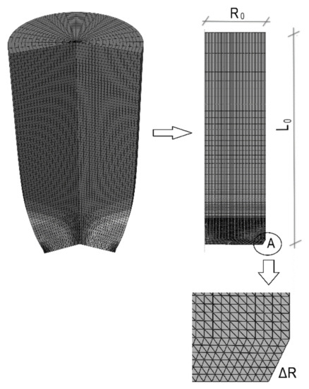
Figure 1.
General geometry and meshing in the first numerical study.
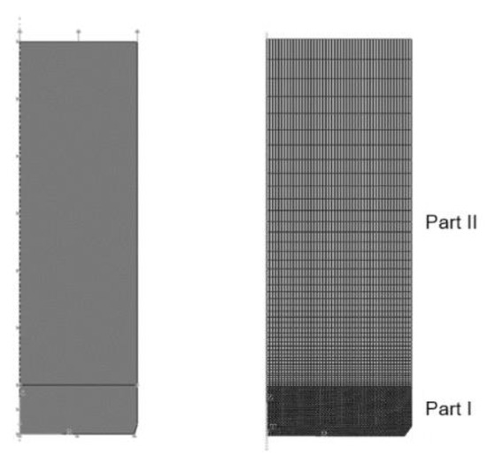
Figure 2.
Kinematic boundary conditions (left) and discretization scheme (right).
In both models, a Young’s modulus of E = 210 GPa, a Poisson’s ratio of ν = 0.3, and a yield point of σpl = 235 MPa have been used [27]. Moreover, the Tvergaard coefficients are considered as equal to , , and . The volume fraction of nucleated voids here is , while the average nucleation strain is assumed as , and the standard deviation of the nucleation strain is [28]. It is known that the Tvergaard coefficients mainly depend on elastic and plastic material properties like the Young’s modulus and yield stress [29]. Figure 3 shows a schematic of the uniaxial behavior of a porous metal (perfectly plastic matrix material with initial volume fraction of voids = f0). The volume fraction of voids existing in the material f0, which is one of the most important parameters in this paper, has been taken as a Gaussian random variable with dispersions of 0.0000–0.0024 and a step size equal to 0.0002. Therefore, in Figure 4, the reduced von Mises stresses obtained for the same global domain with different initial microdefects have been shown. As can be seen, these microdefects affect the overall deformation of the entire specimen to a low degree. This is the reason why their shapes are similar. On the other hand, we can observe that the stress distribution is not equal for all values of f0. The largest values of stress can be observed in total absence of the initial defects (f0 = 0.0). The reduced von Mises stresses are almost constant and equal to the plastic limit before the nucleation phenomenon, whereas they exhibit large variations throughout the values slightly below the yield strength when affected by the micropores. Further computational experiments concerned stochastic analysis and they began with the description of polynomial bases representing local response functions, and this was performed for the extreme horizontal displacements and for von Mises reduced stress localized in the necking area. Maxwell–Huber–Hencky–von Mises theory has been mentioned as being used for von Mises reduced stress. The statistically optimized unweighted least squares method [30] has been used for the determination of these polynomials, precisely at each 10% of the incrementing process expansion. Statistical optimization of the given polynomial basis order means the (i) maximization of the correlation coefficient of the designed polynomial to 13 trial points obtained with the FEM studies obtained for varying values of the randomized parameter about its mean value, and the (ii) minimization of the variance and error of this fitting. This procedure has been carried out using the Taylor–Newton–Gauss algorithm, whose results are given in Table 1 below; it is clear that the eight-order polynomial bases give the most optimal approximation.
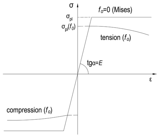
Figure 3.
Schematic of uniaxial behavior of a porous metal (perfectly plastic matrix material with initial volume fraction of voids = f0).
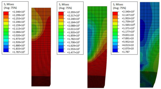
Figure 4.
Reduced von Mises stress distribution (MPa) for f0 = 0.0000, 0.0012, and 0.0024.

Table 1.
Correlation index and RMS error.
The final optimization of these local polynomial response functions are very sensitive to the efficient discretization of the whole domain. As is known from previous simulations, the FEM discretization has a negligible effect on the initial deformations in this necking bar, but on the other hand, a significant effect on the final configuration and possible damage of the extended specimen [20]. The influence of this discretization on the reduced von Mises stresses for various volume fractions of the initial micro-pores has been demonstrated in Figure 4. It is confirmed that these microdefects even with a relatively small volume ratio significantly affect the extreme stresses at the end of the deformation process. Figure 5 shows polynomial response functions for the extreme horizontal displacements as a function of the volume fraction of the voids existing in the material. Some response polynomials for reduced stress are given in Figure 6, and the numerical analysis progress in % is given in the legends of the figures. Such a presentation of the resulting polynomials with parameter f0 given in the X-axis is represented by some variations in the specimen initial voids, which is important in the further stochastic analysis based on partial derivatives with respect to the design input random parameter inherent in Taylor series expansions.
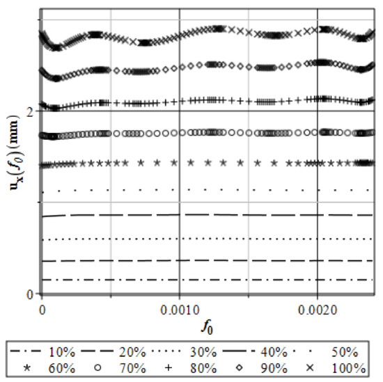
Figure 5.
Response function polynomials of displacements as a function of f0.
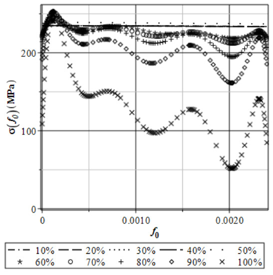
Figure 6.
Response function polynomials for stress as a function of f0.
As can be seen in Figure 5, horizontal displacements ux are almost independent of the void volume fraction f0 variations in a wide range about its given mean value. A confirmation of this fact can be found in numerical values of displacements obtained for the material without the microdefects (f0 = 0.0000), whose values are similar to these computed for extreme voids fraction f0 = 0.0024 in the ABAQUS model. As it can be seen, the model shows a larger sensitivity to initial voids in case of the reduced stress distribution (Figure 6). Starting from these polynomial responses, the first four probabilistic moments of extreme horizontal displacement have been calculated using three concurrent probabilistic numerical techniques—a statistical Monte-Carlo simulation (with 1,000,000 random samples), the nonstatistical generalized perturbation method displayed before, and the semi-analytical method based on integral definitions of the moments and symbolic calculus. All implementations have been provided assuming that the random input is distributed according to the Gaussian probability distribution. These three computer methods have been used for validation and verification of their coincidence (or its lack thereof) for various probabilistic characteristics and for various input uncertainty levels. A computer algebra system MAPLE was used for the implementation of the mentioned methods. The expected values, coefficients of variation, skewness, and kurtosis of the investigated extreme displacements and reduced stress have been computed while randomizing the parameter that specifies the volume of the voids existing in the material f0. Probabilistic moments and characteristics are consecutively determined and plotted for four values of the input coefficient of variation α = [0.05, 0.10, 0.15, 0.20] additionally with the progress of the functions of the FEM incrementing analysis (after each 10% of progress up to its end).
The numerical results section is divided into two parts; first, horizontal displacements are discussed from the statistical point of view, and then the stress analyzed. The expected values of extreme horizontal displacements ux are shown in Figure 7. Through the entire deformation process, displacements monotonously and almost linearly increase. All probabilistic methods coincide perfectly so that these expectations seem to be totally insensitive to the input coefficient of variation. Figure 8 shows the dependence between the input and output coefficient of variation of horizontal displacements in point A. It can be seen that the curves for all probabilistic methods are the same. At an analysis progress of 20%, a local extreme can be observed. The CoV takes values close to zero, which allows us to declare a Gaussian distribution of the deflection state function. Moreover, all output coefficients are about 10 times smaller than the corresponding input one. This confirms the expectations that are strongly concentrated around their means. It can be observed that the imperfect agreement between the statistical and nonstatistical approaches here is the most in the period after 80% of the analysis progress. This situation occurs for the largest input coefficient of variation α = 0.20, which causes some limitation on the perturbation technique here to not be larger than 0.10 when the expectations need to be precisely calculated. The skewness of horizontal displacements (Figure 9) maintain negative values during whole analysis. They are close to zero only if we input a narrow CoV α ≤ 0.05. This assumption is correct for all three conducted methods. For α > 0.05, the skewness tells us about the left-skewed distribution for this state function. Kurtosis of the extreme horizontal displacements of the specimen as a function of the parameter f0 takes both positive and negative values. The biggest negative values kurtosis (Figure 10) takes for perturbation and the Monte–Carlo technique is in the case where α = 0.20. This evidences the flat distribution of displacements in this range. For other values of the input coefficient of variation, all three methods give a kurtosis close to zero. If one bounds an input CoV with α ≤ 0.05, then we can approximate the distribution of this parameter as the Gaussian one.
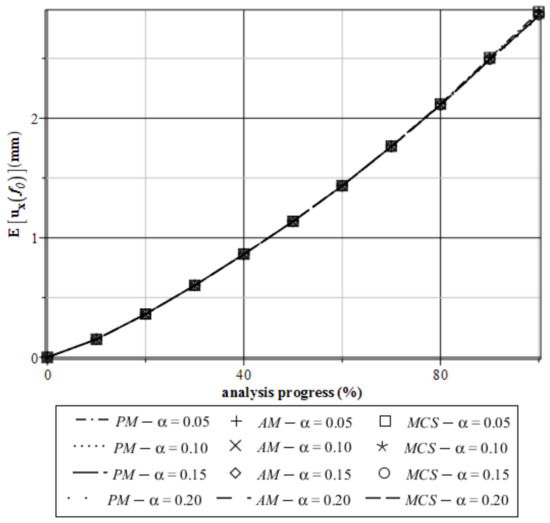
Figure 7.
Expectations of the extreme horizontal displacements E[ux(f0)] for the specimen.
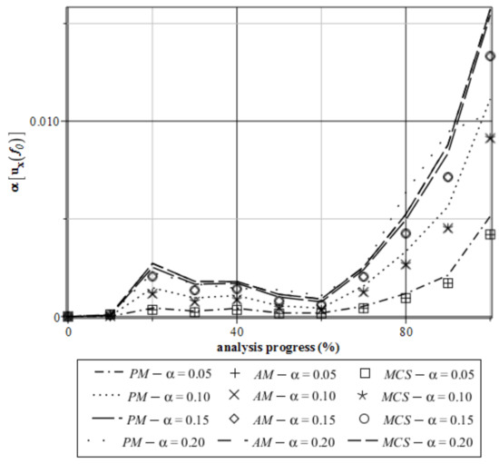
Figure 8.
Coefficient of variation of the extreme horizontal displacements α[ux(f0)] for the specimen.
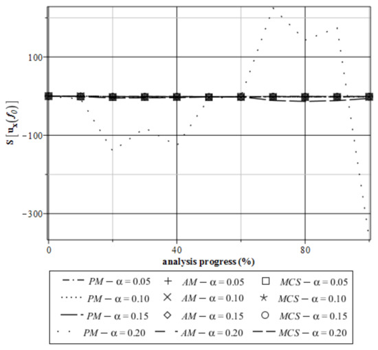
Figure 9.
Skewness of the extreme horizontal displacements S[ux(f0)] for the specimen.
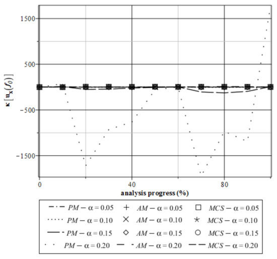
Figure 10.
Kurtosis of the extreme horizontal displacements κ[ux(f0)] for the specimen.
The second part of the computations involves the analysis of the distribution of the reduced von Mises stress. Expectations as a function of the volume fraction of voids existing in the material f0 are shown in Figure 11. Similar displacements for the stress analysis convergence of all three probabilistic methods can be observed. Moreover, we can say that the expectations are completely independent of the input CoV during most of the time of the analysis. After an analysis progress of 80%, small dispersions can be observed. The output coefficient of variation (Figure 12) of the extreme von Mises stress is independent of the used method and input CoV before half of the analysis. At the end of the analysis, the biggest impact of the input CoV can be seen; nevertheless, numerical values of the α[σ(f0)] are always smaller than input one. It tells us about the extreme concentration of expectations around its mean values.
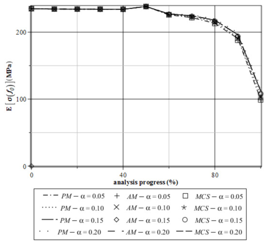
Figure 11.
Expectations of the extreme von Mises stress E[σ(f0)] for the specimen.
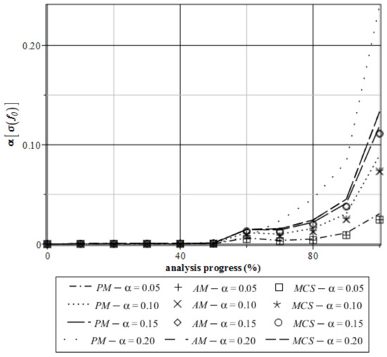
Figure 12.
Coefficient of variation of the extreme von Mises stress α[σ(f0)] for the specimen.
Taking into account the skewness distribution of the stress state function (Figure 13) we can observe a large fluctuation in the Monte–Carlo simulation and α = 0.20. In this case, the skewness reaches values over 60. This means that the range of the input coefficients of variation should be narrowed. The randomization of the initial voids existing in the material has not so large an influence on the skewness for all three methods before half of the analysis. After that, the skewness increases and always takes positive values. Therefore, the stress distribution can be defined as left-modal. Kurtosis of the reduced von Mises stress (Figure 14) shows analogous properties as the skewness. It generally demonstrates large fluctuations from 0 if α = 0.20 for the MCS and AM, but they have different characteristics for various random input variables. The random characteristics of the parameter f0 are best at the end of the analysis. Kurtosis κ[σ(f0)] takes positive and negative values for all three methods. Some fluctuations can be seen at the end of the analysis, but kurtosis is still close to zero. This indicates that expectations are concentrated about the mean values (Figure 11). SFEM analysis of the material with a randomness of its volume fraction of voids f0 also causes different results, so these models can be equivalent in some way, in addition to the correct prediction of the kurtosis of the examined extreme state functions. Analogously to the skewness, a satisfactory agreement of all three probabilistic methods is given if the input coefficient of variation is .
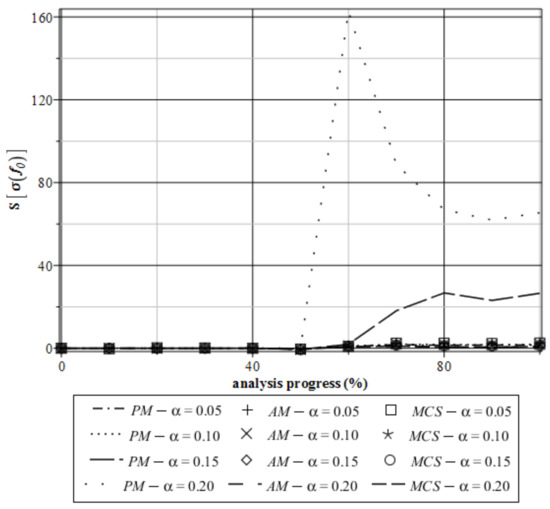
Figure 13.
Skewness of the extreme von Mises stress S[σ(f0)] for the specimen.
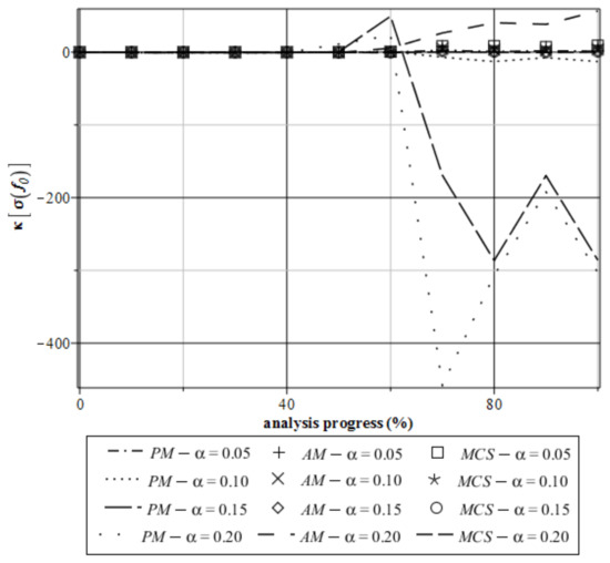
Figure 14.
Kurtosis of the extreme von Mises stress E[σ(f0)] for the specimen.
4. Computer Analysis of Bending Process for the Restrained Steel I-Beam
The subject of the second numerical experiment was a 4 m-long steel I-beam restrained at both its ends with a cross-section shown in the left diagram of Figure 15. Its FEM discretization in the system ABAQUS was completed using 38,000 brick C3D8R finite elements (with reduced integration and hourglass control). This beam was uploaded at its upper flange with a constant pressure equal to 7 kN/m2. The full Newton incremental procedure was applied with the following parameters: initial increment size of 0.0001, minimum set to 0.1, and maximum set as 1.0. The random variable of the problem, initial porosity f0, was defined as the Gaussian variable using its expected value E[f0] = 0.0012, while its CoV belonged to the interval [0.00,0.20]; its range was set to [0.00,0.0024]. The Tvergaard coefficients were adopted here after the first case study as equal to q1 = 1.5, q2 = 1, and q3 = 2.25. Here, the volume fraction of nucleated voids was , while the average nucleation strain was assumed as , and the standard deviation of the nucleation strain was [25]. A Young’s modulus of E = 210 GPa, a Poisson’s ratio of ν = 0.3, and a yield point of σpl = 235 MPa were used in the porous metal plasticity model in ABAQUS. The maps of reduced von Mises stresses, vertical displacements, and void volume fractions computed for the mean value of the initial microvoids ratio are all plotted in Figure 16, Figure 17 and Figure 18, correspondingly. The deformed shape of the given beam is its final configuration after the last increment in this FEM analysis. As one could expect, the largest reduced stresses are obtained in the clamping area, while the extreme displacements are noticed in the middle of the span. The curvature of the deformed shape is not so uniform as for the homogeneous continuous beam, and it is almost negligible in the middle part of this structure. Extreme deformations are observed almost at the restrained ends, and the highest microvoids volume fractions are also noticed in the same location, so that limit state analysis (fundamental for the reliability study) should be based upon static failure scheme with two plastic hinges. One may conclude that the presence of microvoids close to the beams supports may be dangerous for their safety and durability, so the ribs attached to the I-beams at the supports may also reduce the material imperfections.
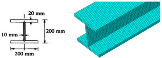
Figure 15.
Cross-sectional dimensions and mesh of the beam.
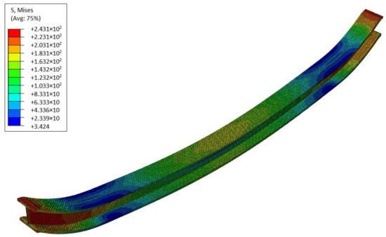
Figure 16.
The reduced von Mises stresses map for the steel beam at the end of the deformation process.
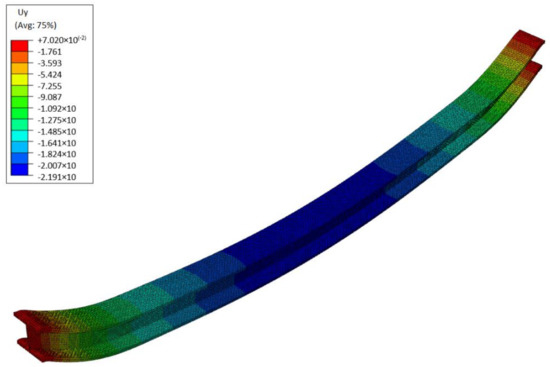
Figure 17.
Vertical displacements map for the steel beam at the end of the deformation process.
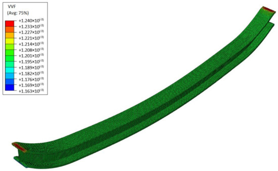
Figure 18.
Void volume fraction map for the steel beam at the end of the deformation process.
The most important part in this test was the determination of the basic probabilistic characteristics of extreme vertical displacements and of the reduced von Mises stresses as a basis for the reliability analysis according to the serviceability and ultimate limit states. This has been provided using three concurrent probabilistic techniques based on the same series of the FEM experiments. These were the Monte–Carlo simulation (abbreviated with MCS below), semi-analytical probabilistic technique (AM), and the generalized stochastic perturbation method (PM). The expected values, coefficients of variation, skewness, and kurtosis of extreme displacements have been collected in Figure 19, Figure 20, Figure 21 and Figure 22, while analogous probabilistic information concerning reduced stresses have been included in Figure 23, Figure 24, Figure 25 and Figure 26. These probabilistic characteristics have been computed for four different statistical scatterings of the input metal porosity α(f0) = 0.05, 0.10, 0.15, 0.20 to demonstrate the influence of the material imperfections uncertainty in this problem. The probabilistic characteristics of interest have all been plotted as functions of the analysis progress varying from 0 to 100% and observed for each 10%.
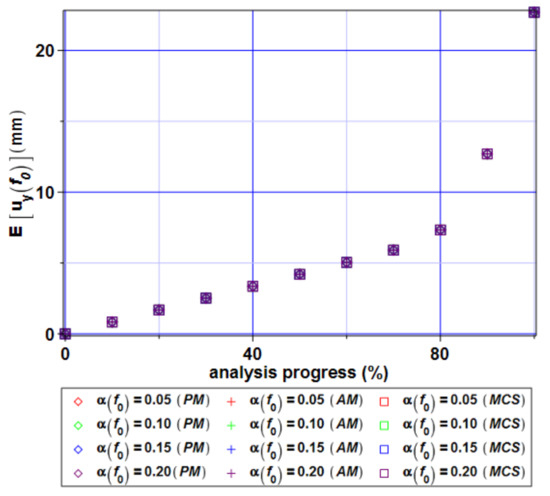
Figure 19.
Expectations of the extreme vertical displacements E[uy(f0)] for the beam.
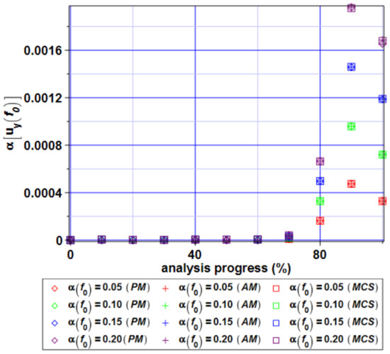
Figure 20.
Coefficient of variation of the extreme vertical displacements α[uy(f0)] for the beam.
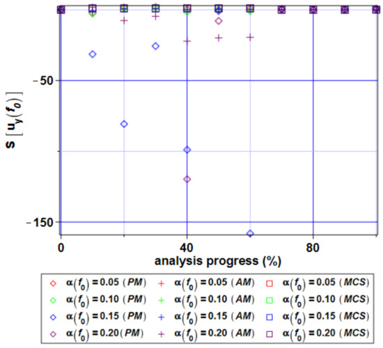
Figure 21.
Skewness of the extreme vertical displacements S[uy(f0)] for the beam.
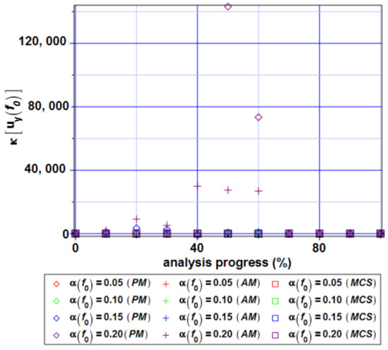
Figure 22.
Kurtosis of the extreme vertical displacements κ[uy(f0)] for the beam.
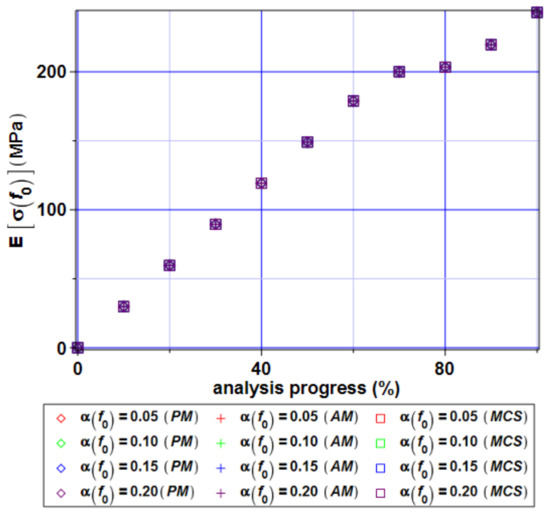
Figure 23.
Expectations of the extreme von Mises stress E[σ(f0)] for the beam.
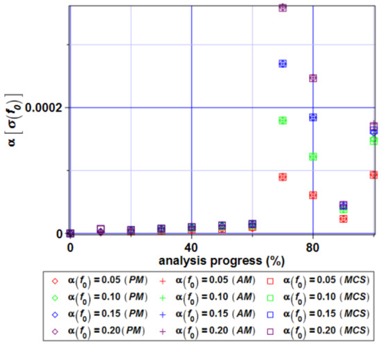
Figure 24.
Coefficient of variation of the extreme von Mises stress α[σ(f0)] for the beam.
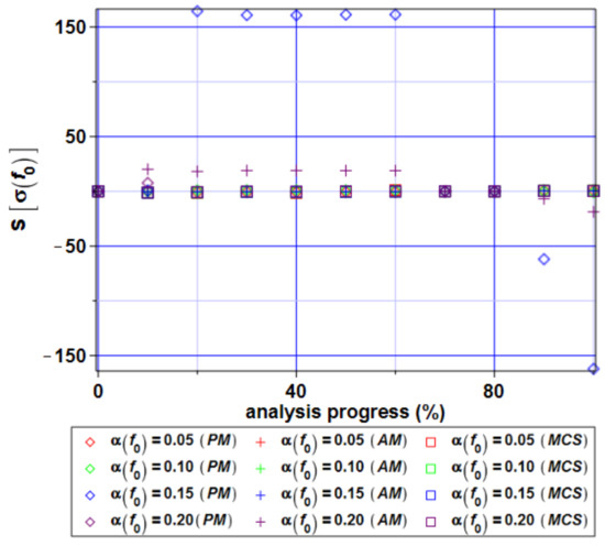
Figure 25.
Skewness of the extreme von Mises stress S[σ(f0)] for the beam.
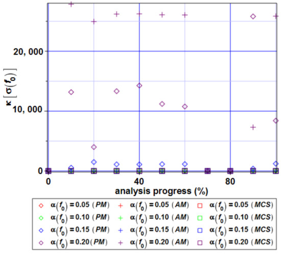
Figure 26.
Kurtosis of the extreme von Mises stress κ[σ(f0)] for the beam.
It can be noticed that the expected values of both displacements and reduced stresses systematically increase throughout the uploading process. Large variations are observed in the case of the displacements at the end of this process, where the reduced stresses exhibit some fluctuations. All three probabilistic numerical techniques coincide perfectly in the case of the expectations independent of the nonlinear analysis stage. Additionally, the input scattering level has practically no impact on the resulting expected values.
Almost the same perfect coincidence is obtained for the output CoV, whose values in both structural responses (cf. Figure 20 and Figure 24) are marginal. Nevertheless, an input uncertainty level starts to remarkably affect the resulting coefficients of variation when the analysis progress reaches 60–70%.
Higher-order statistics do not show a good coincidence, especially in-between the stochastic perturbation method and the remaining two reference numerical techniques. Both the skewness and kurtosis of extreme displacements estimated with the use of the Monte–Carlo simulation technique stay very close to 0, which means that the resulting probability distribution is similar to the Gaussian one; these obtained with the PM approach may take huge negative and positive values, respectively, and do not indicate the same conclusion. It is important to mention that the largest absolute values of kurtosis for both displacements and stresses are obtained with α(f0) = 0.05, which may be a result of some numerical discrepancies appearing at very small uncertainty levels. The skewness exhibits some variations independently of this level and very frequently shows the lack of coincidence of different probabilistic numerical methods. One can generally notice here that the uncertainty in the microvoids plays a secondary role here; more important is the deterministic fact of their presence, especially close to the supports of this beam.
Probabilistic moments of the first and the second order have been combined into the reliability indices for the serviceability limit state (Figure 27) and, independently, for the ultimate limit state (Figure 28). They have been plotted in the same manner as above— for different uncertainty levels of the microvoids (α(f0) = 0.05, 0.10, 0.15, 0.20)—and also as a function of nonlinear deformation progress. The reference value depicted in Eurocode 0 has been inserted in both figures to determine the critical analysis level, where this structure can be qualified as unreliable. In both cases, the reliability indices decrease very fast together with the advancement of the uploading process in an exponential way in the case of the reduced stresses and with some initial variations, when the SLS is analyzed. Contrary to the previous diagrams, the influence of the material microvoids uncertainty is remarkable and some differences in-between the resulting indices β computed for various values of α(f0) are noticeable. It is seen that the critical state is the SLS here, where minimum admissible values of the reliability index is reached just before 40% of nonlinear analysis progress, while the ULS indicates a slightly larger steel I-beam capacity here. It should be underlined that the FORM reliability assessment usually brings more optimistic results than the SORM or higher-order methods [31], so the realistically admissible uploading level may be even smaller; however, the FORM approach has been applied and discussed here as the one included in the Eurocode 0 designing demands.
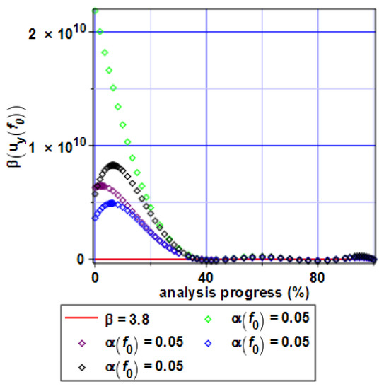
Figure 27.
Reliability index for the serviceability limit state (extreme vertical displacement) for the beam.
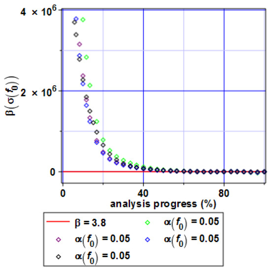
Figure 28.
Reliability index of the ultimate limit state (extreme von Mises stress) for the beam.
5. Conclusions
The iterative generalized stochastic perturbation approach has been applied in this paper for the numerical simulation of an elasto-plastic material with stochastic microvoids. It has been implemented as the 10th-order stochastic finite element method to compute the first four probabilistic characteristics of the structural response thanks to the interoperability of the FEM system ABAQUS and computer algebra system MAPLE 2019. The constitutive model for structural carbon steel adopted here was the Gurson–Tvergaard–Needleman metal plasticity [32], where a volume fraction of the initial microvoids existing in the material f0 was randomized in both case studies according to the Gaussian distribution with a fixed expected value and with some variability in the coefficient of variation. A comparison of the fundamental probabilistic characteristics with these estimated via the Monte–Carlo simulation and, independently, with these integrated using the semi-analytical approach has been included. The numerical results obtained in this work generally confirm the usage of a higher-order stochastic perturbation technique to model elasto-plastic phenomena with large deformations and stochastic structural micro-defects. The computer simulation based on the Taylor series stochastic perturbation technique can be a very efficient alternative for the well-known Monte–Carlo simulation for the entire deformation processes of steel materials and structures in the case of the expected values and variances of structural responses. A reliable determination of the first two probabilistic moments also needs some bounds on the input coefficient of variation of uncertain parameters, and it can be proposed here as set to α ≤ 0.10; the efficient determination of higher probabilistic characteristics (as skewness or kurtosis) may demand larger restrictions in this context, like α ≤ 0.05. Further SFEM analyses may be extended on the post-necking strain hardening behavior of the steel elements with microstructure uncertainty. However, the extension of the presented study to include more advanced constitutive models (Johnson–Cook, Ramberg–Osgood, or Hill material constitutive model), symmetric but non-Gaussian probability distributions (like triangular or uniform), as well as the usage of nonsymmetric probability distributions (log-normal, Gumbel, Weibull) and the straightforward application of the generalized stochastic perturbation method could be interesting analyses in the future.
Author Contributions
M.K.; conceived and designed the experiments, M.S.; performed the experiments and analyzed the data, M.K. and M.S.; contributed the materials and analysis tools, M.K. and M.S.; both wrote the entire paper. All authors have read and agreed to the published version of the manuscript.
Funding
Not applicable.
Institutional Review Board Statement
Not applicable.
Informed Consent Statement
Not applicable.
Data Availability Statement
Not applicable.
Conflicts of Interest
The authors declare no conflict of interest.
References
- Rahimidehgolan, F.; Majzoobi, G.; Alinejad, F.; Sola, J.F. Determination of the Constants of GTN Damage Model Using Experiment, Polynomial regression and Kriging Methods. Appl. Sci. 2017, 7, 11. [Google Scholar] [CrossRef]
- Strąkowski, M.; Kamiński, M. Stochastic Finite Element Method elasto-plastic analysis of the necking bar with material microdefects. ASCE ASME J. Risk Uncert. Eng. Sys. Part B Mech. Eng. 2019, 5, 030908. [Google Scholar] [CrossRef]
- Franklin, A.G. Comparison between a Quantitative Microscope and Chemical Methods for Assessment of Non-Metallic Inclusions. J. Iron Steel Inst. 1969, 207, 181–186. [Google Scholar]
- Dormieux, L.; Kondo, D. An extension of Gurson model incorporating interface stresses effects. Int. J. Eng. Sc. 2010, 48, 575–581. [Google Scholar] [CrossRef]
- Tvergaard, V.; Needleman, A. Analysis of the cup-cone fracture in a round tensile bar. Act. Metall. 1984, 32, 157–169. [Google Scholar] [CrossRef]
- Malcher, L.; Reis, F.J.P.; Andrade Pires, F.M.; César de Sá, J.M.A. Evaluation of shear mechanisms and influence of the calibration point on the numerical results of the GTN model. Int. J. Mech. Sci. 2013, 75, 407–422. [Google Scholar] [CrossRef]
- Buryachenko, V. Elastic-plastic behavior of elastically homogeneous materials with a random field of inclusions. Int. J. Plast. 1999, 15, 687–720. [Google Scholar] [CrossRef]
- Kleiber, M.; Hien, T.D. The Stochastic Finite Element Method: Basic Perturbation Technique and Computational Implementation; Wiley: Chichester, UK, 1992. [Google Scholar]
- Kamiński, M. Probabilistic characterization of porous plasticity in solids. Mech. Res. Comm. 1999, 26, 99–106. [Google Scholar] [CrossRef]
- Kamiński, M. On the dual Iterative Stochastic perturbation-based Finite Element Method in solid mechanics with Gaussian uncertainties. Int. J. Num. Meth. Eng. 2015, 104, 1038–1060. [Google Scholar] [CrossRef]
- Oh, C.K.; Kim, Y.J.; Baek, J.H.; Kim, Y.P.; Kim, W. A phenomenological model of ductile fracture for API X65 steel. Int. J. Mech. Sci. 2007, 49, 1399–1412. [Google Scholar] [CrossRef]
- Kossakowski, P. Analysis of the void volume fraction for S235JR steel at failure for low initial stress triaxiality. Arch. Civ. Eng. 2018, 64, 101–115. [Google Scholar] [CrossRef]
- Johnson, G.R.; Cook, W.H. Fracture characteristics of three metals subjected to various strains, strain rates, temperatures and pressures. Eng. Fract. Mech. 1985, 21, 31–48. [Google Scholar] [CrossRef]
- Boyer, J.C.; Vidal-Salle, E.; Staub, C. A shear stress dependent ductile damage models. Int. J. Mater. Process. Technol. 2003, 121, 87–93. [Google Scholar] [CrossRef]
- Weck, A.; Seguarado, J.; Lorca, J.L.; Wilkinson, D. Numerical simulations of void linkage in model materials using a nonlocal ductile damage approximation. Int. J. Fract. 2007, 148, 205–219. [Google Scholar] [CrossRef][Green Version]
- Aravas, N. On the numerical integration of a class of pressure-dependent plasticity models. Int. J. Num. Meth. Eng. 1987, 24, 1395–1416. [Google Scholar] [CrossRef]
- Morin, L.; Kondo, D.; Leblond, J.-B. Numerical assessment, implementation and application of an extended Gurson model accounting for void size effects. Euro. J. Mech. Sol. 2015, 51, 183–192. [Google Scholar] [CrossRef]
- Kleiber, M.; Woźniak, C. Nonlinear Mechanics of Structures; Kluwer Academic Publishers: Dordrecht, The Netherlands, 1991. [Google Scholar]
- Oden, J.T. Finite Elements of Nonlinear Continua; McGraw-Hill: New York, NY, USA, 1972. [Google Scholar]
- Kossakowski, P. The numerical modeling of failure of 235JR steel using Gurson-Tvergaard-Needleman material model. Roads Bridges 2012, 11, 295–310. [Google Scholar]
- Ockewitz, A.; Sun, D.-Z. Damage modeling of automobile components of aluminum materials under crash loading. In Proceedings of the LS-DYNA Anwenderforum, Ulm, Germany, 12–13 October 2006. [Google Scholar]
- Tvergaard, V. Influence of voids on shear band instabilities under plane strain conditions. Int. J. Frac. 1981, 17, 389–407. [Google Scholar] [CrossRef]
- Zhou, J.; Gao, X.; Sobotka, J.C.; Webler, B.A.; Cockerman, B.V. On the extension of the Gurson-type porous plasticity models for prediction of ductile fracture under shear-dominated conditions. Int. J. Sol. Struct. 2014, 51, 3273–3291. [Google Scholar] [CrossRef]
- Kamiński, M.; Świta, P. Generalized stochastic finite element method in elastic stability problems. Comp. Struc. 2011, 89, 1241–1252. [Google Scholar] [CrossRef]
- Kamiński, M. The Stochastic Perturbation Method for Computational Mechanics; Wiley: Chichester, UK, 2013. [Google Scholar]
- Zienkiewicz, O.C.; Taylor, R.C. The Finite Element Method, 4th ed.; McGraw Hill: New York, NY, USA, 1989. [Google Scholar]
- EN 1993-1-1:2005. Eurocode 3: Design of Steel Structures-Part 1-1: General Rules and Rules for Buildings; CEN/European Committee for Standardization: Brussels, Belgium, 2005.
- Oh, Y.R.; Kim, J.S.; Kim, Y.-J. Determination Damage Parameters for Application to Pipe Ductile Fracture Simulation. Proc. Eng. 2015, 130, 845–852. [Google Scholar] [CrossRef][Green Version]
- Wciślik, W. Experimental determination of critical void volume fraction fF for the Gurson Tvergaard Needleman (GTN) model. Proc. Struct. Integ. 2016, 2, 1676–1683. [Google Scholar] [CrossRef]
- Bjorck, A. Numerical Methods for Least Squares Problems; SIAM: Philadelphia, PA, USA, 1996. [Google Scholar]
- Melchers, R.E. Structural Reliability Analysis and Prediction; Wiley: Chichester, UK, 2002. [Google Scholar]
- Leblond, J.-B.; Morin, L.; Cazacu, O. An improved description of spherical void growth in plastic porous materials with finite porosities. Proc. Mat. Sc. 2014, 3, 1232–1237. [Google Scholar] [CrossRef]


Publisher’s Note: MDPI stays neutral with regard to jurisdictional claims in published maps and institutional affiliations. |
© 2021 by the authors. Licensee MDPI, Basel, Switzerland. This article is an open access article distributed under the terms and conditions of the Creative Commons Attribution (CC BY) license (https://creativecommons.org/licenses/by/4.0/).