
Adaptive First Principles Model for the CAS-OB Process for Real-Time Applications


Abstract
:1. Introduction
2. Materials and Methods
2.1. Control Volumes and State-Space Variables
2.1.1. Liquid Steel Phases
2.1.2. Slag Phase
2.1.3. Gas Phase
2.1.4. Ladle
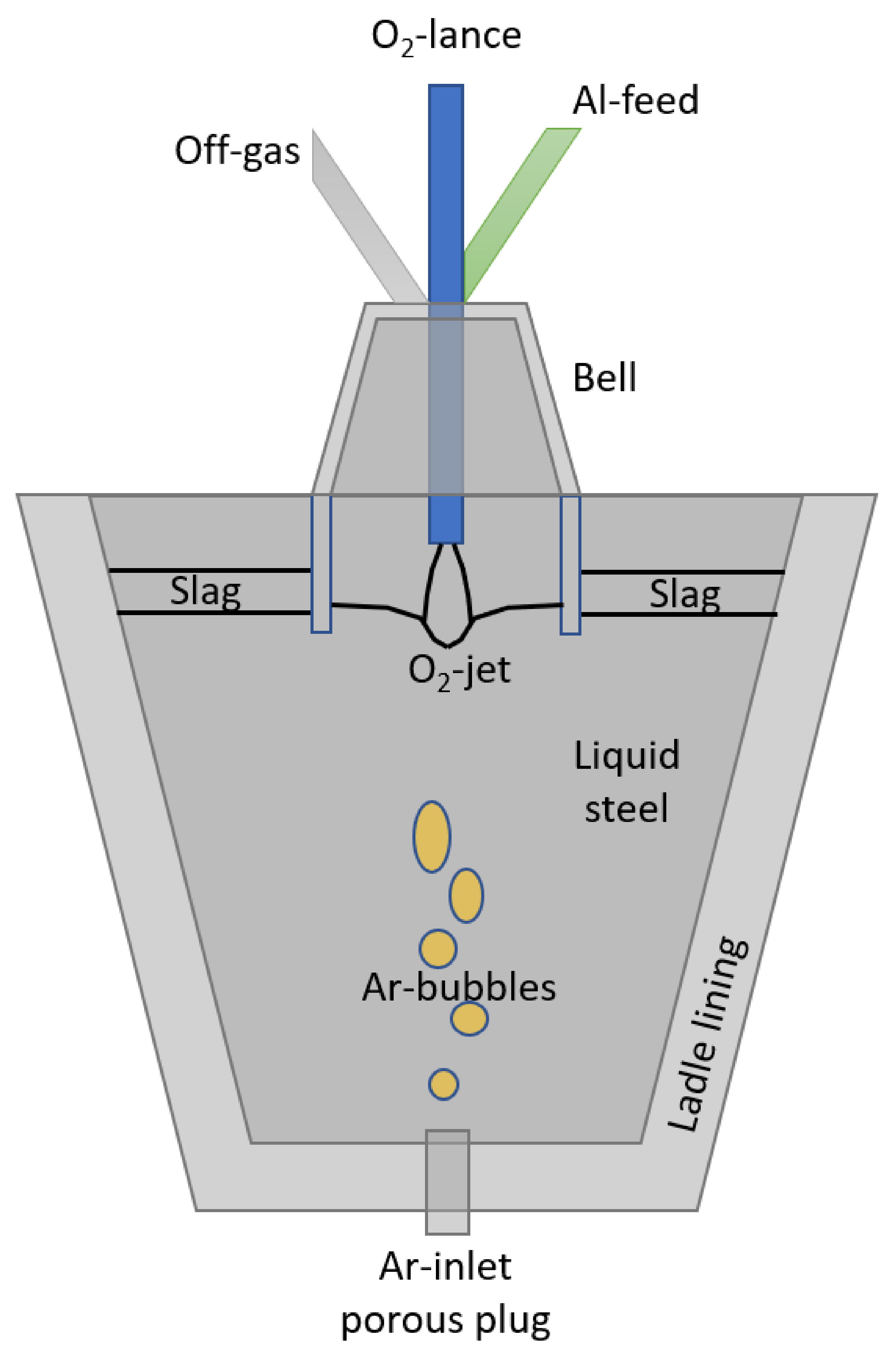
2.1.5. Bell
2.2. Chemical Reactions
2.2.1. Dissolution of Added Material
2.2.2. Free Surface Reactions
2.2.3. Slag-Metal Interface Reactions
2.3. Heat Transfer
2.4. Mass and Energy Balances
2.4.1. Free Surface
2.4.2. Liquid Steel
2.4.3. Gas Phase
2.4.4. Model Summary
2.5. Recursive Parameter and State Estimation
2.6. Real-Time Optimization

3. Results
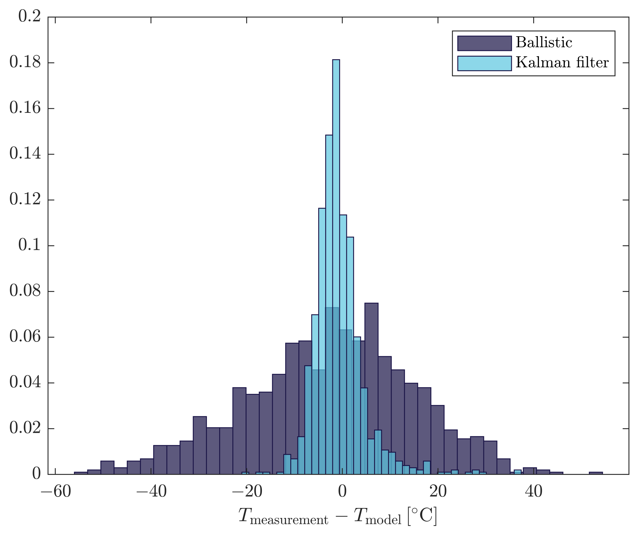
3.1. Model Agreement with Process Data
3.2. Recursive Estimation
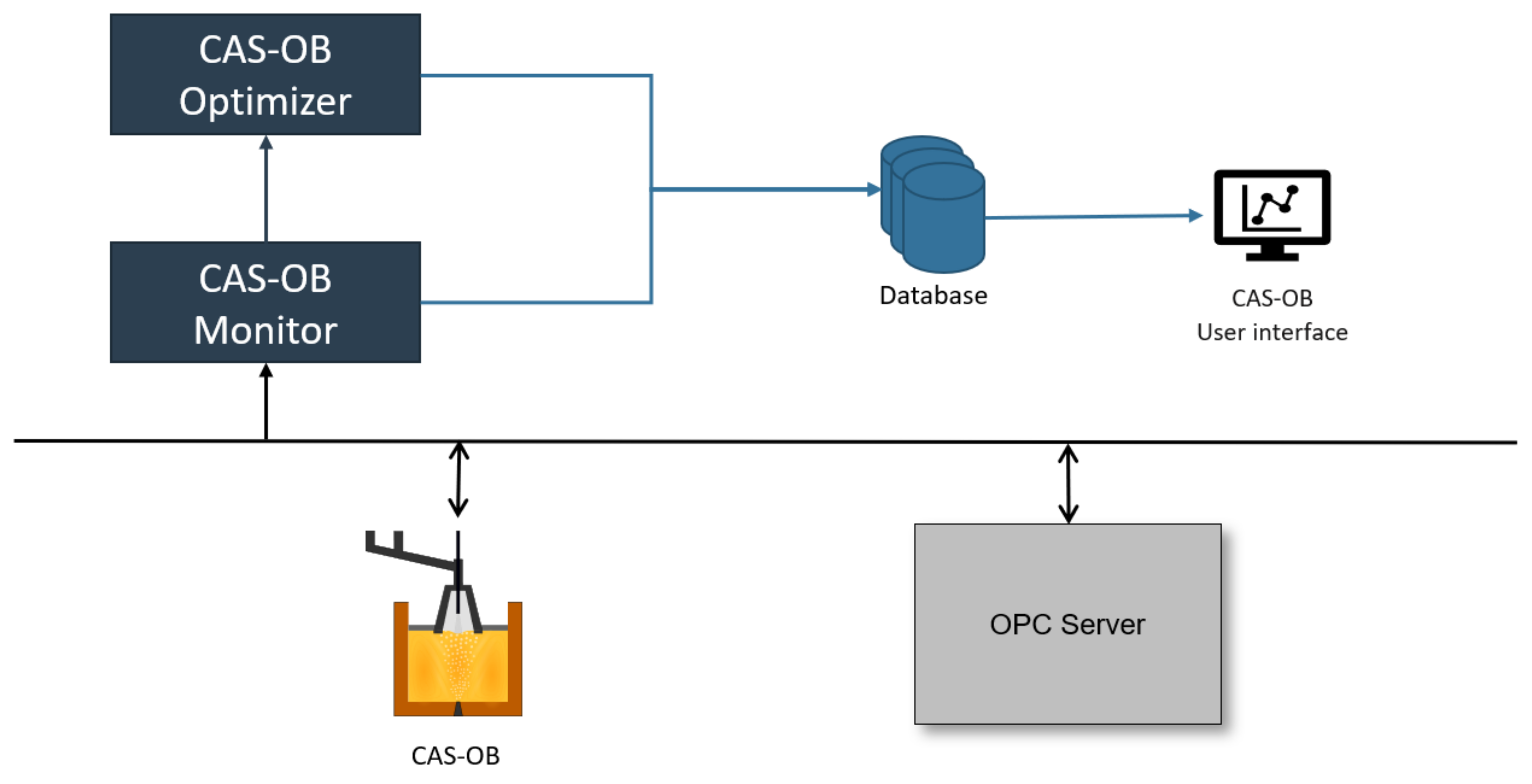
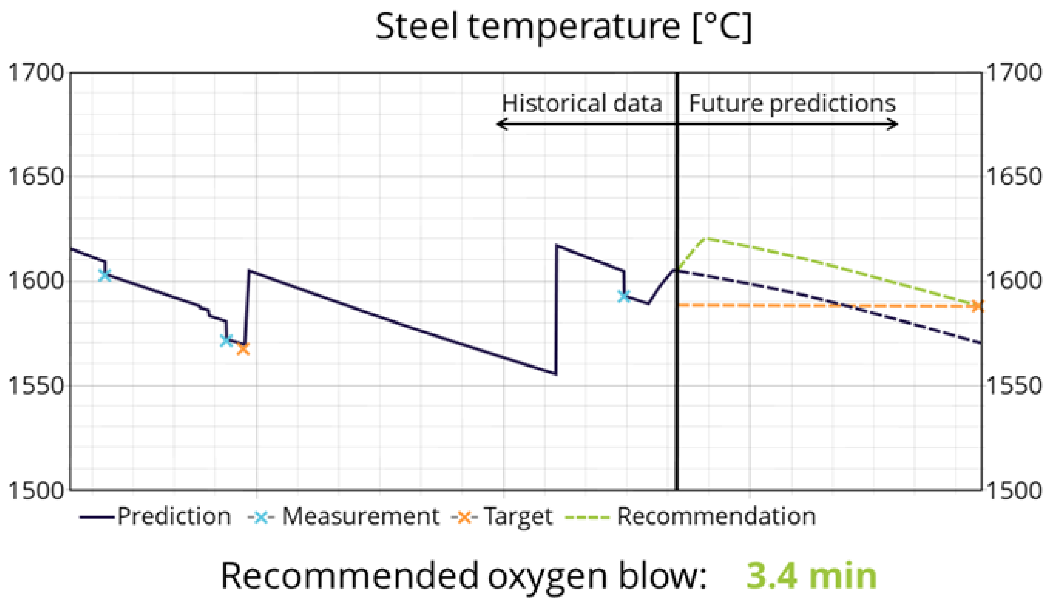
3.3. Industrial Use and Application
4. Conclusions
Author Contributions
Funding
Institutional Review Board Statement
Informed Consent Statement
Acknowledgments
Conflicts of Interest
Abbreviations
| BOF | Basic Oxygen Furnace | |
| CAS-OB | Composition Adjustment by Sealed | |
| argon-bubbling with Oxygen Blowing | ||
| CFD | Computational Fluid Dynamics | |
| MPC | Model Predictive Control | |
| NMPC | Nonlinear Model Predictive Control | |
| Symbol | Description | Unit |
| Mass of component i | kg | |
| Concentration of component i | mass fraction | |
| Specific molar mass of component i | kg/kmol | |
| Mass flow of component i | kg/s | |
| Reaction rate of reaction j | kmol/s | |
| Temperature of control volume k | K | |
| Heat transfer between control volumes k and l | W | |
| Heat capacity of component or control volume | J/(kg K) | |
| Surface area of k | m | |
| Heat transfer coefficient for k | W/(m K) | |
| Subscript notation | ||
| f | Free surface control volume | |
| L | Liquid control volume | |
| Inner section of Ladle control volume | ||
| Inner section of Bell control volume | ||
| s | Slag control volume | |
| f–L | From Free surface to Liquid control volumes | |
| L–f | From Liquid to Free surface control volumes | |
| Material addition |
References
- Ollila, S.; Syrjänen, A.; Robey, R. Commissioning and Initial Results from New Twin CAS-OB Plant at Ruukki, Raahe Steel Works. In Proceedings of the 6th European Oxygen Steelmaking Conference (EOSC), Stockholm, Sweden, 7–9 September 2011; pp. 170–183. [Google Scholar]
- Järvinen, M.; Kärnä, A.; Ollila, S.; Fabritius, T. A novel approach for numerical modeling of the CAS-OB process. In Proceedings of the Scanmet IV, Luleå, Sweden, 10–13 June 2012; pp. 79–88. [Google Scholar]
- Fruehan, R.J. (Ed.) The Making, Shaping and Treating of Steel; The AISE Steel Foundation: Pittsburgh, PA, USA, 1998; ISBN 0-930767-02-0. [Google Scholar]
- Ghosh, A. Secondary Steelmaking, Principles and Applications; CRC Press: Boca Raton, FL, USA, 2001; ISBN 978-0-849-30264-0. [Google Scholar]
- Rotevatn, T.; Wasbø, S.; Järvinen, M.; Fabritius, T.; Ollila, S.; Hammervold, A.; Blasio, C.D. A Model of the CAS-OB Process for Online Applications. In Proceedings of the Preprints of the IFAC 4th Workshop on Mining, Minerals and Metal Processing, Oulu, Finland; 2015. [Google Scholar]
- Sulasalmi, P.; Visuri, V.V.; Kärnä, A.; Järvinen, M.; Ollila, S.; Fabritius, T. A Mathematical Model for the Reduction Stage of the CAS-OB Process. Metall. Trans. B 2016, 47, 3544–3556. [Google Scholar] [CrossRef]
- Visuri, V.V.; Järvinen, M.; Pääskylä, K.; Kärnä, A.; Sulasalmi, P.; DeBlasio, C.; Ollila, S.; Fabritius, T. Preliminary Validation of a Numerical Model for the CAS-OB Process. In Proceedings of the 7th European Oxygen Steelmaking Conference (EOSC), Třinec, Czech Republic, 9–11 September 2014. [Google Scholar]
- Kärnä, A.; Järvinen, M.; Sulasalmi, P.; Visuri, V.V.; Ollila, S.; Fabritius, T. An Improved Model for the Heat-Up Stage of the CAS-OB Process: Development and Validation. Steel Res. Int. 2018, 89, 1800141-16. [Google Scholar] [CrossRef]
- Schei, T.S. On-line estimation for process control and optimization applications. J. Process. Control 2008, 18, 821–828. [Google Scholar] [CrossRef]
- Simon, D. Optimal State Estimation: Kalman, H Infinity, and Nonlinear Approaches; Wiley: Hoboken, NJ, USA, 2006; ISBN 978-0-471-70858-2. [Google Scholar]
- Maciejowski, J.M. Predictive Control With Constraints; Prentice Hall: Boston, MA, USA, 2002; ISBN 978-0-201-39823-6. [Google Scholar]


Publisher’s Note: MDPI stays neutral with regard to jurisdictional claims in published maps and institutional affiliations. |
© 2021 by the authors. Licensee MDPI, Basel, Switzerland. This article is an open access article distributed under the terms and conditions of the Creative Commons Attribution (CC BY) license (https://creativecommons.org/licenses/by/4.0/).
Share and Cite
Linnestad, K.; Ollila, S.; Wasbø, S.O.; Bogdanoff, A.; Rotevatn, T. Adaptive First Principles Model for the CAS-OB Process for Real-Time Applications. Metals 2021, 11, 1554. https://doi.org/10.3390/met11101554
Linnestad K, Ollila S, Wasbø SO, Bogdanoff A, Rotevatn T. Adaptive First Principles Model for the CAS-OB Process for Real-Time Applications. Metals. 2021; 11(10):1554. https://doi.org/10.3390/met11101554
Chicago/Turabian StyleLinnestad, Kasper, Seppo Ollila, Stein O. Wasbø, Agne Bogdanoff, and Torstein Rotevatn. 2021. "Adaptive First Principles Model for the CAS-OB Process for Real-Time Applications" Metals 11, no. 10: 1554. https://doi.org/10.3390/met11101554
APA StyleLinnestad, K., Ollila, S., Wasbø, S. O., Bogdanoff, A., & Rotevatn, T. (2021). Adaptive First Principles Model for the CAS-OB Process for Real-Time Applications. Metals, 11(10), 1554. https://doi.org/10.3390/met11101554