Elastoplastic Fracture Analysis of the P91 Steel Welded Joint under Repair Welding Thermal Shock Based on XFEM

Abstract

P91 steel is a typical steel used in the manufacture of boilers in ultra-supercritical power plants and heat exchangers in nuclear power plants. For the long-term serviced P91 steel pressurized structures, the main failure mode is the welded joint failure, especially the heat affected zone (HAZ) failure. Repair welding technique is an effective method for repairing such local defects. However, the thermal shock composed of high temperature and thermal stress in the repair welding process will pose a critical loading condition for the existing defects near the heat source which cannot be detected by conventional means. So, the evaluation of structural integrity for the welded joint in the thermal-mechanical coupling field is necessary. In this work, the crack propagation law in the HAZ for the P91 steel welded joint was investigated under repair welding thermal loads. The weld repair model of the P91 steel welded joint was established by ABAQUS. The transient temperature field and stress field in repair welding process were calculated by relevant user subroutines and sequential coupling simulation method. The residual stress was determined by the impact indentation strain method to verify the feasibility of the finite element (FE) model and simulation method. In order to obtain the crack propagation path, the elastoplastic fracture analysis of the welded joint with initial crack was performed based on the extended finite element method (XFEM). The influence of different welding linear energy on the crack propagation was analyzed. The results show that the cracks in the HAZ propagate perpendicular to the surface and tend to deflect to the welding seam under repair welding thermal loads. The crack propagation occurs in the early stage of cooling. Higher welding linear energy leads to larger HAZ and higher overall temperature. With the increase of welding linear energy, the length and critical distance of the crack propagation increase. Therefore, low welding linear energy can effectively inhibit the crack propagation in the HAZ. The above calculation and analysis provide a reference for the thermal shock damage analysis of repair welding process, which is of great significance to improving the safety and reliability of weld repaired components.

1. Introduction

P91 steel is widely used in boiler components of ultra-supercritical power plants due to its excellent creep strength and steam corrosion resistance at high temperature [1]. It is also one of the common choices of steel pipe material for heat exchangers in nuclear power plants [2]. In practical application, P91 steel is usually connected by welding to form the pressure equipment components. During long-term service, local defects will occur inevitably in pressure equipment due to the effect of harsh service environment or improper operation procedure, especially in vulnerable parts, such as welded joints [3,4]. As a Cr-Mo heat-resistant steel, the main failure mode of the P91 steel welded joints is the type IV cracking near the fine-grained zone (FGHAZ) (shown in Figure 1), which will result in the degradation of structural safety [5]. An efficient and economic method to repair the cracking region is to remove the area with local defects and then refill it with welding rods by repair welding technique [6,7], which greatly extends the service life of pressure equipment. However, conventional defect detection means, including radiographic testing, ultrasonic testing, magnetic particle testing, penetrant testing and eddy current testing, have a corresponding detection sensitivity. This will result in undetected defects existing in the structure.

Repair welding is a rapid welding heat transfer process, and the arc temperature during welding process may reach thousands of degrees centigrade [8]. The welding heat source loads a large amount of heat flow into the welding seam and nearby area in a short time. The high temperature and the unsteady thermal stress act on the weldment in the form of thermal shock. On the one hand, it will cause the formation of hot cracks in the welding seam; on the other hand, the interaction between existing cracks and thermal-mechanical coupling field will lead to the crack propagation and even the failure of the whole component. In order to ameliorate the quality of weldments and weld repaired components, it is necessary to study the effect of the welding process on the cracking behavior. Alvarez et al. [9] compared the hot cracking sensitivity of tungsten inert gas welding (TIG) and laser beam welding (LBW) by analyzing the microstructure and chemical composition of the welding seam of 718 alloy. Chelladurai et al. [10] studied the solidification cracking behavior of 316 stainless steel under different energy transfer modes by adjusting the pulse parameters in pulsed laser welding (PLW). Hosseini et al. [11] investigated the effect of heat input and welding speed in electron beam welding (EBW) on the hot cracking sensitivity of AA2024-T351 alloy experimentally. Coniglio et al. [12] explored the initiation mechanism of solidification crack in the arc welding seam for 6060 aluminum alloy theoretically and numerically. Wei et al. [13] developed a software which can automatically plot the driving force and resistance curves of solidification cracks according to the numerical and experimental results. Bordreuil et al. [14] established a solidification cracking model which can predict microstructure and pore nucleation in the welding seam by combining cellular automata model with intergranular fluid flow model. Agarwal et al. [15] analyzed the influence of metallurgical factors and molten pool shape on the solidification cracking in laser beam welding of advanced high strength steels numerically and experimentally. Jiang et al. [16] researched the effect of repair width on residual stress for the composite plate to reduce the probability of interface cracking. Hyde et al. [17] studied the creep crack propagation behavior of P91 steel weldment under constant loads by both experimental method and finite element (FE) method. Pandey et al. [18] investigated experimentally the effect of different diffusible hydrogen concentrations in weld metal on hydrogen-induced cracking features of P91 steel. Zhang et al. [19] applied the high energy spark deposition (HESD) method to weld repair and tested the fracture properties of the repair welding seam. He et al. [20] performed the elastic fracture analysis of cracked aluminum alloy plate during metal inert gas welding (MIG) and cooling processes.

According to the existing literature, a lot of theoretical and experimental studies have been carried out on the hot cracks in welding processes. Almost all the current numerical simulations of cracking behavior for welding focus on the structure without crack or with stationary crack. The thermal effect of welding, especially repair welding, will make the existing cracks which are neglected by conventional detection methods further extend and even penetrate through the whole structure. However, there is little research on the crack propagation behavior under repair welding thermal shock. Therefore, it is necessary to analyze the structural integrity of weldments under repair welding thermal loads.

Combined with the specific damage model, the extended finite element method (XFEM) can simulate the ductile crack growth behavior accurately [21]. Belytschko [22] first proposed the embryonic form of the XEFM. It was independent of mesh generation and enhanced the finite element approximation by adding discontinuous enrichment functions to the displacement field near the crack tip. Moës et al. [23] introduced the step function and crack tip asymptotic function to describe the crack surface and crack tip, respectively, making it successfully used in the analysis of fracture mechanics, and called this technique “extended finite element method”. Daux et al. [24] added several different asymptotic functions and step functions to the crack tip and crack surface to simulate the crack branching. Chessa et al. [25] improved the convergence of the blending element in the XFEM (shown in Figure 2) by utilizing the extended strain method. Stolarska et al. [26] used the level set method to locate the crack location, which further improved the theory of the XFEM. For completing the modelling of dynamic crack, Song et al. [27] applied the phantom node method to the XFEM, which implemented the definition of the crack propagation behavior within the framework of the conventional finite element method. Until now, FE software such as ABAQUS, ANSYS and LS-DYNA have implemented the XFEM program into the function module of fracture analysis. This paper uses the XFEM to predict how the repair welding thermal shock affects the cracking behavior of the heat affected zone (HAZ) in a P91 steel welded joint. The influence of welding linear energy on the cracking features has been studied, which provides a reference for repair welding of structures containing defects. This study has guiding significance for the life extension of pressure equipment under long-term service or extended service.

2. FE Model and Simulation Method

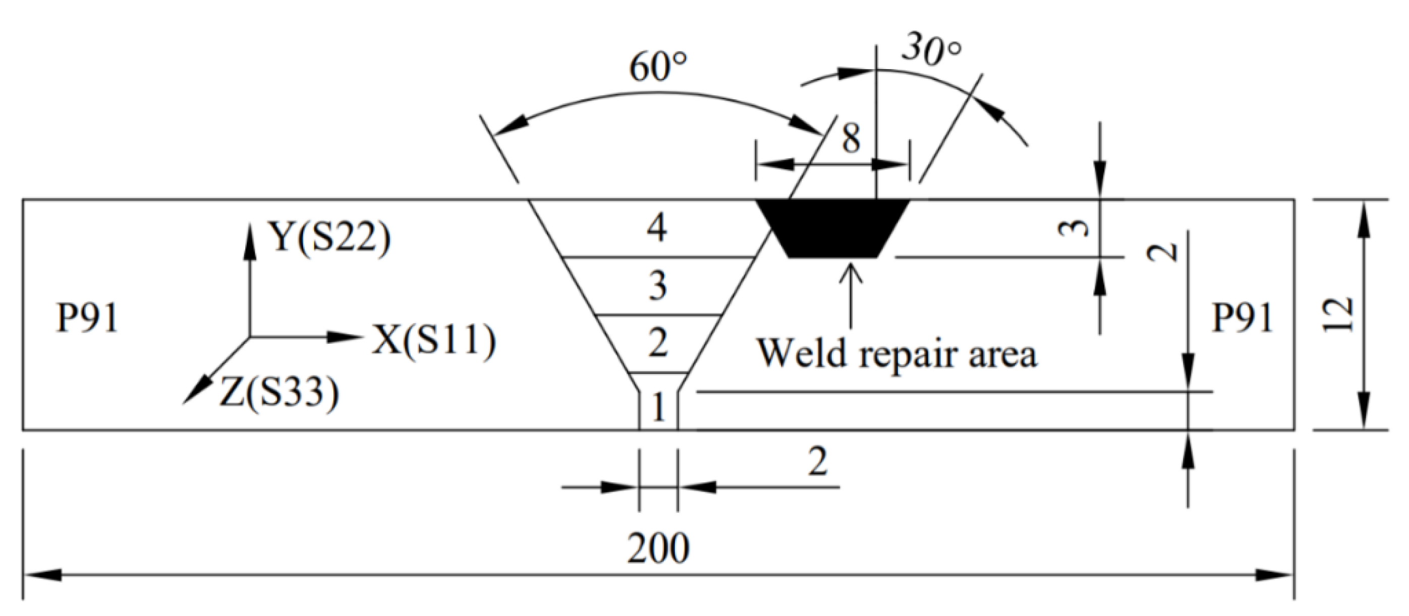
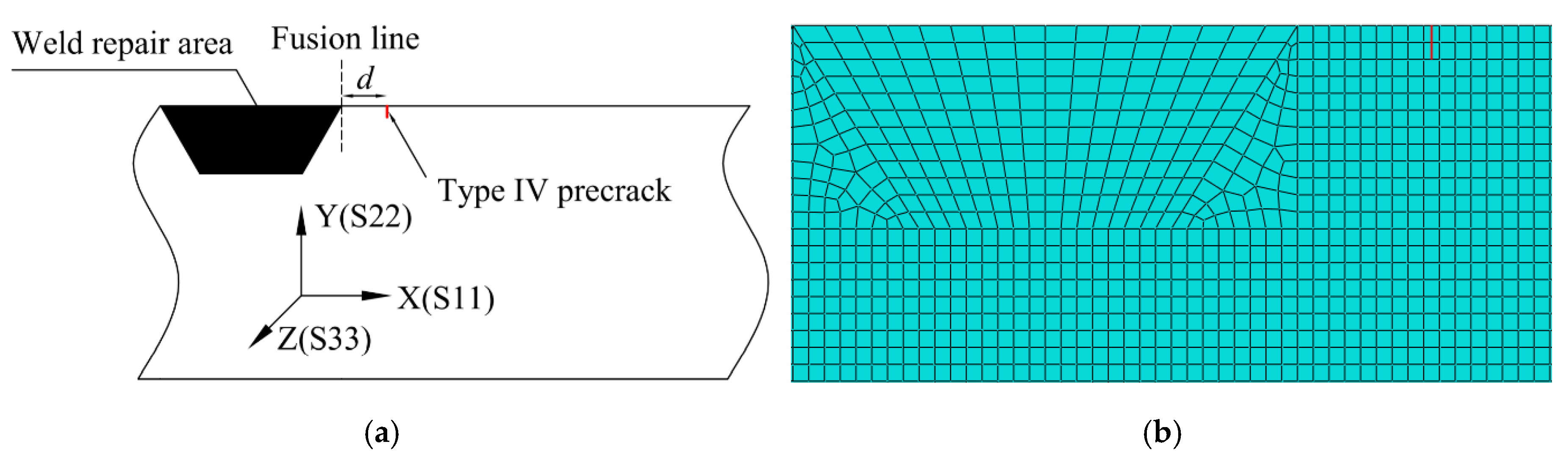
2.1. Model Geometry

Two P91 steel plates with a size of 200 mm × 100 mm × 12 mm (length, width and thickness, respectively) are butt welded with four welding layers, including two layers of root welding (welding layers 1 to 2), one layer of filler welding (welding layer 3) and one layer of cover welding (welding layer 4). The selection of the form and size of welding groove is based on the criteria of Yang et al. [28]. A V-shaped groove is adopted, the root gap and blunt edge are both 2 mm, the groove angle is 60°. The area containing a type IV crack in the HAZ will be removed and then refilled by repair welding. The size of weld repair area is 80 mm × 8 mm × 3 mm (length, width and thickness, respectively), and the angle of groove surface for repair welding is 30°. Figure 3 shows the schematic drawing of the model geometric dimensions.

The finite element modelling tool of thermal-mechanical coupling process and fracture behavior is ABAQUS 6.14-5 (Dassault Systemes, Paris, France). In order to save the calculating work and avoid the convergence problem in 3-D computational fracture mechanics, a 2-D plane strain analysis model is set up. The plane studied in this paper is the middle cross section of the plate, as shown in Figure 4. Mesh refinement is carried out in the welding seam and HAZ, where exist high heat flux loading, to overcome the mesh-sensitivity problem. The area far away from the welding seam and HAZ is coarsened appropriately to reduce the calculation time. The transitional mesh is adopted between the refined mesh and the coarsened mesh. The FE model and meshing are shown in Figure 5. A total of 9063 elements and 9322 nodes are meshed. The element edge size for the refined mesh is 0.25 mm, and that for the coarsened mesh is 2 mm.

The sequential coupling method is used in the thermal-mechanical coupling simulation. Firstly, the thermal analysis is performed, and then the temperature field results are applied to the nodes of the mechanical model to carry out the mechanical analysis. The removal and deposition of the metal are implemented by the method of Birth and Death Element. A 4-node linear heat transfer quadrilateral (DC2D4) element is adopted for the thermal analysis, and a 4-node bilinear plane strain quadrilateral reduced-integration (CPE4R) element is adopted for the mechanical analysis. The topological relationship for meshing between the thermal model and the mechanical model is consistent.

2.2. Material Properties and Heat Source Model

2.2.1. Material Property

Temperature-dependent nonlinear features are considered for the thermal physical properties and mechanical properties of P91 steel, as shown in Figure 6. The thermal physical properties include thermal conductivity, specific heat and thermal expansion coefficient, while the mechanical properties include Young’s modulus, Poisson’s ratio and yield strength. The density of P91 steel is assumed to be constant at a value of 7780 kg/m³. The material properties of the weld metal are also considered in the FE simulation for obtaining higher accuracy. The solidus and liquidus temperatures of both base metal and weld metal are set at 1420 °C and 1500 °C, respectively. The melting heat and solidification heat of the material are both set at 260 kJ/kg.

2.2.2. Heat Source Definition

The heat source loads should reflect the actual temperature change during welding as accurately as possible. The distributed heat flux (DFLUX) has been widely used because of its mature theory. Among the distributed heat flux, Gaussian heat flux distribution, uniform body heat flux distribution and double ellipsoidal heat flux distribution are commonly used [30].

The thermal exchange during welding is mainly the thermal conduction inside the weldment, which follows Fourier’s law (Equation (1)), and the governing equation of temperature field (Equation (2)) follows the law of conservation of energy.

$$R=-\lambda \times \frac{\partial T}{\partial x}$$

(1)

$$\rho c\times \frac{\partial T}{\partial t}=\frac{\partial }{\partial x}\times \left(\lambda \times \frac{\partial T}{\partial x}\right)+\frac{\partial }{\partial y}\times \left(\lambda \times \frac{\partial T}{\partial y}\right)+\frac{\partial }{\partial z}\times \left(\lambda \times \frac{\partial T}{\partial z}\right)+Q$$

(2)

where:

• R is the heat flux (W/m²);
• λ is the thermal conductivity (W/m·k);
• T is the distribution function of temperature field (K);
• ρ is the density (kg/m³);
• c is the specific heat (J/kg·K);
• t is the transient time (s);
• Q is the intensity of thermal energy (W), including the thermal energy generated by the heat source and the thermal energy generated by the solid-liquid phase change.

The conventional uniform body heat flux distribution is defined by Equation (3) [29].

$$q=\frac{\eta \times U\times I}{V_{act}}$$

(3)

where q is the heat generation rate by heat source; η is the arc efficiency factor; U is the arc voltage; I is the welding current; V_act is the action volume of the heat source.

The conventional uniform body heat flux distribution adopts amplitude curves to control the piecewise changes of the heat generation rate with time. The forms of the changes are linear in each time segment, which cannot reflect the real situation of the heat source passing through the plane. In addition, the value of V_act needs to be estimated first and then calibrated according to the experimental results. Continuous adjustment must be made until the simulated results are consistent with the experimental results.

An improved uniform body heat flux distribution is used to simulate the welding process. The action volume of the heat source is calculated according to the groove size and welding process parameters. As shown in Figure 7, assuming that all thermal energy is concentrated in the filler metal, V_act is determined by the product of the cross-sectional area of the welding layer (A) and the action length of the heat source (C). C is estimated by Equation (4) [31].

$$C=\tau \times U\times I$$

(4)

where τ is the coefficient determined by the welding method and welding process parameters, and in this paper τ = 3 mm·kW⁻¹.

Therefore, the total action time of the heat source is obtained by Equation (5).

$$t_{act}=\frac{C}{v}=\frac{\tau \times U\times I}{v}$$

(5)

where v is the welding speed.

Considering the effect of the heat source approaching and leaving the studied cross section during the welding process, the improved uniform body heat flux distribution changes with time instantaneously. The distributed heat flux is calculated by Equation (6) [32].

$$q=\frac{\eta \times U\times I}{V_{act}}\exp \left\{\frac{-12\times {\left[v\times \left(t-t_0\right)\right]}^2}{C^2}\right\}$$

(6)

where t is the transient loading time; t₀ is the time taken for the center of the heat source to move to the studied cross section, equal to half of t_act.

The modelling of the improved uniform body heat flux distribution is done by FORTRAN language written in DFLUX, one of user subroutines in ABAQUS. The arc efficiency factor is assumed to be 0.8 for the shielded metal arc welding (SMAW), and 0.6 for the gas tungsten arc welding (GTAW).

2.3. Boundary Conditions

The ambient temperature is assumed as 20 °C. The convection heat transfer exists between air and weldment surface during welding due to the temperature difference. Additionally, the temperature difference between weldment surface and surrounding environment will result in continuous radiation heat transfer. The convection heat transfer follows Newton’s law of cooling (Equation (7)).

$$q_c={\alpha }_c\times \Delta T$$

(7)

where q_c is the heat flux of convection heat transfer; α_c is the convection heat transfer coefficient; ΔT is the value of temperature difference between air and weldment surface.

The convection heat transfer coefficient is calculated by Equation (8), which is introduced into the FE model by the user subroutine FILM in ABAQUS 6.14-5.

$${\alpha }_c=\{\begin{array}{cc}0.0668\times T\hfill & 0<T\le 500{}^{°}\mathrm{C}\\ 0.231T-82.1\hfill & T>500{}^{°}\mathrm{C}\end{array}$$

(8)

where T is the transient temperature of the weldment surface.

The heat flux radiated outward by weldment follows the Stefan–Boltzmann law (Equation (9)).

$$q=\epsilon \times \sigma \times T^4$$

(9)

where ε is the emissivity, assumed as 0.85; σ is the Stefan-Boltzmann constant with the value of 5.67 × 10⁻⁸ W/m²·K⁴. T is the temperature of the weldment surface.

The radiation heat transfer between weldment surface and surrounding environment is calculated by Equations (10) and (11).

$$q_r={\alpha }_r\times \left(T-T_f\right)$$

(10)

$${\alpha }_r=\epsilon \times \sigma \times \frac{{\left(\frac{T+273}{100}\right)}^3-{\left(\frac{T+273}{100}\right)}^4}{T-T_f}$$

(11)

where q_r is the heat flux of radiation heat transfer; α_r is the radiation heat transfer coefficient; T_f is the ambient temperature.

During the mechanical analysis, degrees of freedom for node A and node B at two ends of the bottom surface of the FE model (shown in Figure 5) are constrained in the X direction and Y direction to prevent the rigid body displacement.

2.4. Thermal Loading Patterns

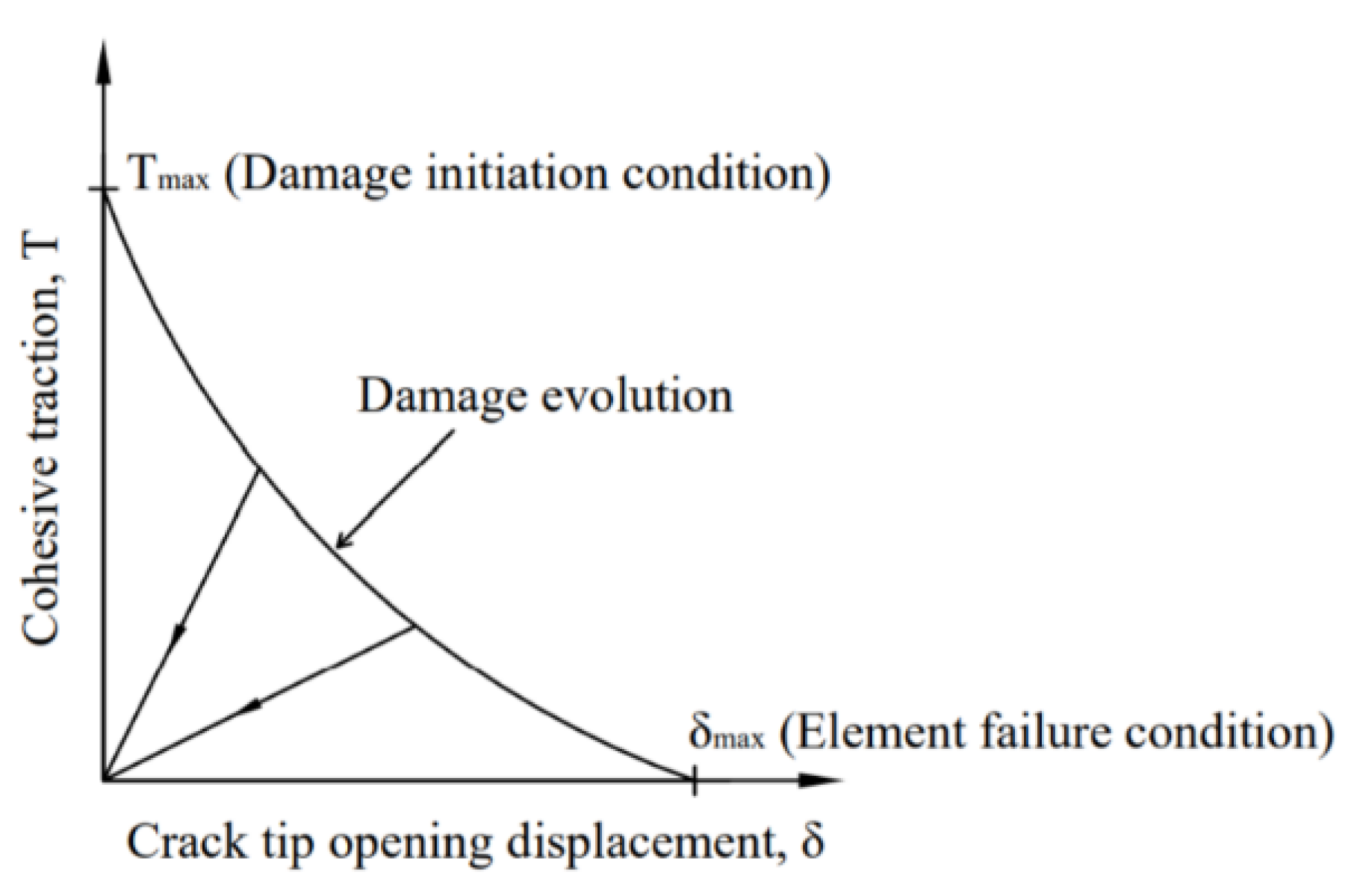
Welding linear energy is the heat energy input by welding heat source to unit length welding seam, which influences the surface forming of welding seam and the formation of welding defects. The magnitude of welding linear energy is calculated by Equation (12).

$$Q=\frac{\eta \times U\times I}{v}$$

(12)

Three different repair welding linear energy levels will be considered in the fracture analysis. The values of three selected linear energies are 10 kJ/cm, 16 kJ/cm and 25 kJ/cm, respectively. According to the heat flux distribution defined by Equation (6), the time distribution curves of heat generation rate in the weld repair area under three different linear energy rates is plotted in Figure 8. The heat generation rate presents a Gaussian profile with time, which can reflect the moving features of the heat source. With the increase of linear energy, both the duration of the thermal loading and the generated total heat energy increase. The duration of the thermal loading is 3.96 s for the linear energy of 10 kJ/cm, 6.34 s for the linear energy of 16 kJ/cm and 9.90 s for the linear energy of 25 kJ/cm. All three thermal loading patterns have the same peak heat generation rate in the intermediate instant of the corresponding loading time, which is 14.8 GW/m³. The intermediate instant is the time when the center of the heat source passes through the studied cross section.

2.5. Damage Model

The XFEM used in this paper is based on the cohesive crack model [33]. The damage response of a crack takes the traction–separation law as the constitutive relation. As shown in Figure 9, the damage development includes three stages: damage initiation, damage evolution and element failure.

The damage initiation of a crack is the starting point at which the cohesive stiffness between the crack surfaces begins to degrade. It occurs when the stress or strain of the element reaches a critical value. Here, the maximum principal stress (MPS) criterion is used to judge whether a crack reaches the damage initiation condition. Meanwhile, the crack propagation direction is also controlled by the MPS criterion. The cohesive crack will propagate along the direction of maximum principal stress. The damage initiation criterion satisfies Equation (13).

$$1\le f=\frac{\langle {\sigma }_{\max }\rangle }{{\sigma }_{\max }^0}\le 1+f_{\mathrm{tol}}$$

(13)

where < σ_max > is the actual maximum principal stress of the element, the symbol “< >“ means the damage initiation does not exist in a pure compression state; ${\sigma }_{\max }^0$ is the allowable maximum principal stress defined; f_tol is the tolerance with a value of 0.05, which is a default value recommended by ABAQUS.

The damage evolution defines the degradation patterns of cohesive stiffness after damage initiation. The nonlinear exponential softening response is adopted to describe the degradation of cohesive stiffness for the analysis of elastoplastic fracture mechanics (EPFM). As the fracture energy is one of the fracture properties of materials, the evolution law based on energy method is selected. Once the crack propagation driving force exceeds the equivalent critical energy release rate (equivalent to fracture energy), the crack will extend. The equivalent critical energy release rate is calculated by the Benzeggagh–Kenane law (Equation (14)) [34].

$$G_{eqC}=\left(G_{IIC}-G_{IC}\right)\times {\left(\frac{G_{II}+G_{III}}{G_I+G_{II}+G_{III}}\right)}^{\eta }+G_{IC}$$

(14)

where G_eqC is the equivalent critical energy release rate; G_I, G_II and G_III are the energy release rates of mode I, II and III cracks, respectively; G_IC and G_IIC are the critical energy release rates of mode I and II cracks, respectively; η is the exponent, to which the response is insensitive for isotropic failure.

Fracture toughness is an index to measure the capacity of materials to prevent crack propagation, which is one of the inherent properties of materials. It can be expressed by a single parameter such as energy release rate G, stress intensity factor K, crack tip opening displacement CTOD and J-integral. The critical energy release rate is used as the fracture toughness here. The fracture failure mode is assumed to be isotropic, so G_IC = G_IIC. The fracture energy in the process of damage evolution is calculated on the basis of the fracture toughness of P91 steel. The tensile strength of P91 steel is taken as an approximation for the MPS. For both fracture toughness and tensile strength, temperature-dependent data are used to simulate the actual fracture behavior. The fracture parameters under high temperature are extrapolated by a linear interpolation method. The fracture properties of P91 steel are shown in Figure 10.

With the development of damage evolution, the cohesive traction between crack surfaces decreases. When the cohesive traction is reduced to zero, the element fails, which means that the crack surfaces have been completely opened.

The fracture problems with damage definition have strong nonlinearity and discontinuity, which makes numerical solutions difficult to converge. ABAQUS provides a viscous regularization method to solve this problem. By setting an appropriate small viscosity coefficient, the convergence of the fracture model will be significantly improved. Here, the viscosity coefficient is set to be 1.0 × 10⁻⁵.

The type IV crack with a size of 0.5 mm perpendicular to the surface is prefabricated in the HAZ of repair welding, as shown in Figure 11a. d is the distance between the crack and the fusion line. The initial crack is introduced into the FE model by the XFEM technique, and the contact attributes between the crack surfaces are set as frictionless for tangential behavior and “hard” contact for normal behavior, as shown in Figure 11b.

3. Weld Repair Experiments

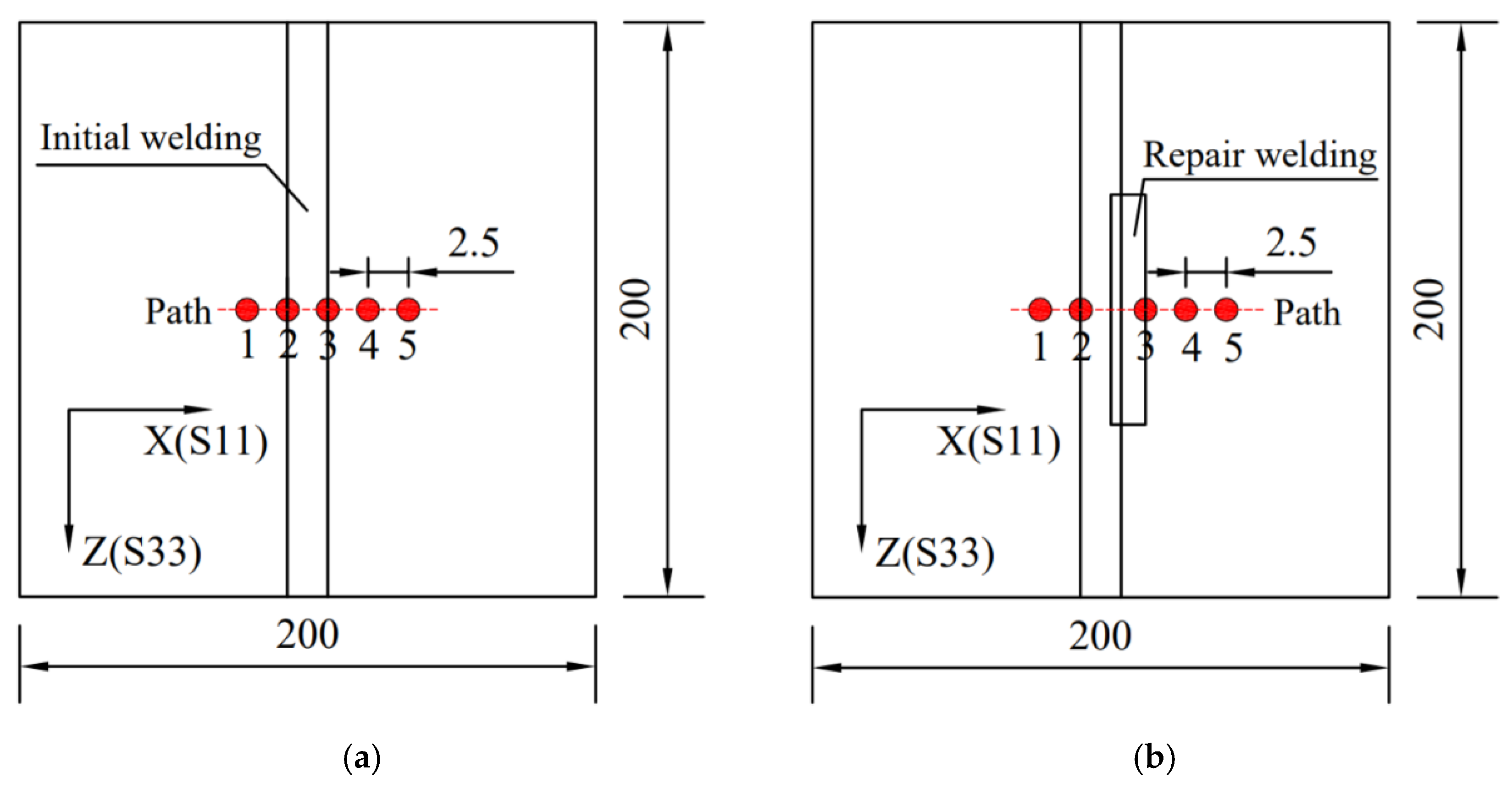
3.1. Weld Repair Specimens

Weld repair experiments of the P91 steel welded joint were carried out to verify the feasibility of the FE model. The size of the specimens was the same as that of the FE model. The chemical composition of experimental base metal is shown in

Table 1. Chemical composition of P91 steel (wt. %).

C	Si	Mn	S	P	Cr	Ni	Mo	V	Nb	N	Al
0.08	0.27	0.6	0.006	0.007	8.86	0.38	0.98	0.19	0.06	0.06	0.04

, which measures up to ASME BPVC.II.A-2019 [37]. The selected weld metal was particularly suited for matching P91 steel. ER90S-B9 welding rod was used as a filler metal for GTAW, while E9015-B9 stick electrode was used as a filler metal for SMAW. The chemical composition of the weld metal is shown in

Table 2. Chemical composition of the weld metal (wt. %).

Material Grade	C	Si	Mn	Cr	Ni	Mo	V	Nb
ER90S-B9	0.1	0.3	0.5	9.0	0.7	1.0	0.2	0.06
E9015-B9	0.09	0.2	0.6	9.0	0.8	1.1	0.2	0.05

, which measures up to ASME BPVC.II.C-2019 [38].

Firstly, the base metal plates were connected by multilayer welding. GTAW was used for root welding, followed by SMAW used for filler welding and cover welding. The shielding gas for GTAW was argon. Then the welded joint was air-cooled to the ambient temperature. The metal near the FGHAZ of the welded joint, where it was prone to IV type cracking, was removed. Finally, repair welding technique was utilized to refill it by SMAW with the welding linear energy of 10 kJ/cm. The specific welding parameters for each layer and weld repair are shown in

Table 3. Specific welding parameters for each layer and weld repair.

Layer Number	Welding Method	Electrode Grade	Electrode Diameter (mm)	Welding Current (A)	Arc Voltage (V)	Welding Speed (cm/min)
1	GTAW	ER90S-B9	2.4	100	12	6
2	GTAW	ER90S-B9	2.4	110	14	6
3	SMAW	E9015-B9	3.2	110	20	12
4	SMAW	E9015-B9	3.2	120	22	12
Repair	SMAW	E9015-B9	3.2	120	22	12

. The interlayer temperature was maintained at 200–300 °C during welding. The morphology of welding seams after initial welding and repair welding is shown in Figure 12.

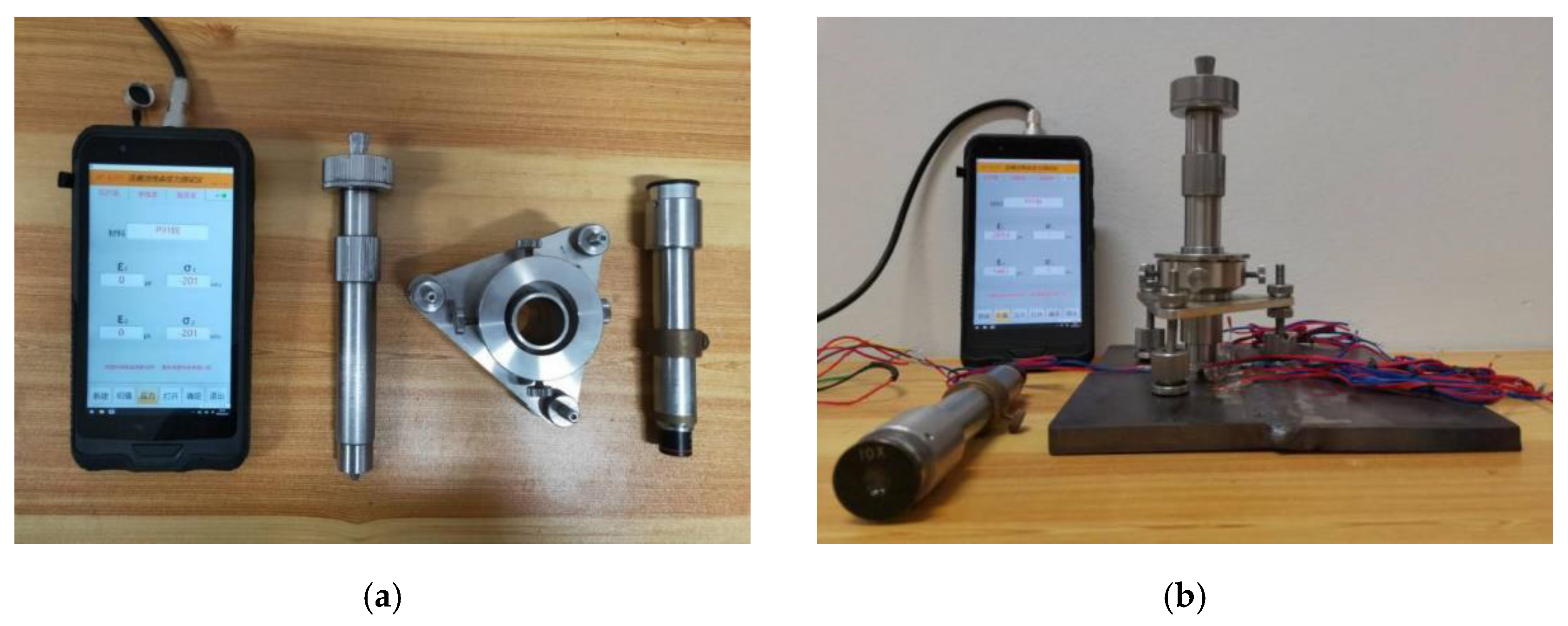
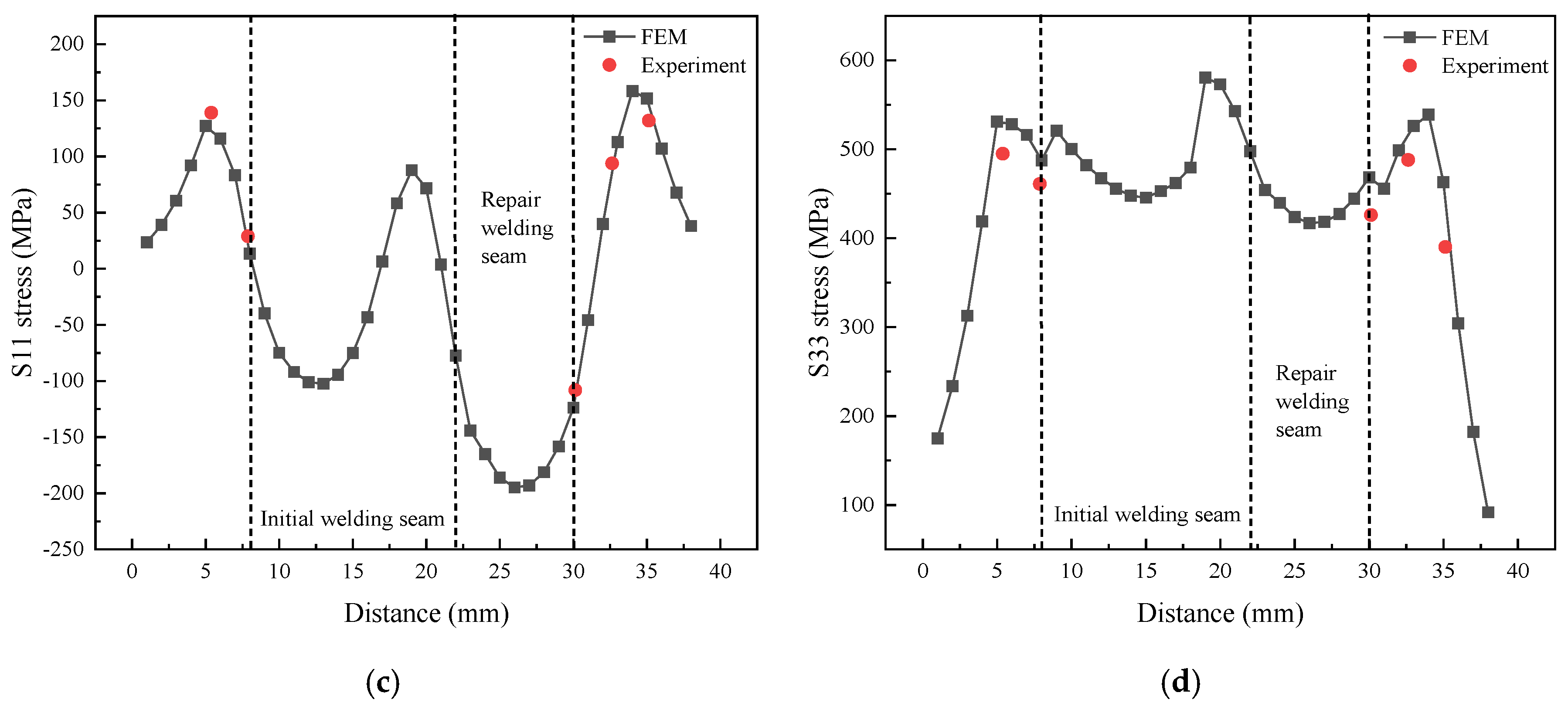
3.2. Verification of the FE Model

After the fabrication of weld repair specimens, the impact indentation strain method [39] was used to measure the residual stress. A spherical indenter was used to generate indentations in the form of impact loads at the location of measuring points. On the one hand, the impact action makes the material appear to have plastic flow deformation. On the other hand, the elastoplastic deformation caused by indentations itself changes under the action of residual stress. The total deformation after superposition of the two kinds of deformation is called strain increment. The relationship between the strain increment generated by the impact indentation strain method and elastic strain satisfies Equation (15).

$$\Delta \epsilon =a_1\times {\epsilon }_e+a_2\times {\epsilon }_e{}^2+a_3\times {\epsilon }_e{}^3+B$$

(15)

where Δε is the strain increment; ε_e is the elastic strain; a₁, a₂, a₃ are the coefficients obtained from the calibration curve; B is the strain increment in a zero-stress state.

The biaxial resistance strain gauge containing two sensing grid elements with different axial directions, namely X-axis direction and Z-axis direction, was used to measure residual strain. A certain size of indentation was produced at the midpoint of the grid axis by the impact load. The value of strain increment was recorded by the strain recording instrument. The value of residual strain was determined according to the relationship between the calibrated elastic strain and the strain increment. The value of residual stress was calculated by Hooke’s law.

The surface residual stress of specimens after both initial welding and repair welding was measured. Five measuring points were taken from each specimen, and the distance between adjacent measuring points on each side of the welding seam was 2.5 mm. The specific position of each measuring point is shown in Figure 13. The measurement of surface residual stress was finished by the KJS-3\4 indentation stress measurement system (Developed by Institute of Metal Research, Chinese Academy of Sciences, Shenyang, China). Before measurements, the accuracy of the indentation stress measurement system was calibrated with conventional residual stress measurement methods, such as X-ray diffraction, which measures up to GB/T 24179-2009. As shown in Figure 14a, the measurement system consists of two parts: portable intelligent stress tester and indentation generating device. The indentation generating device includes a striking rod (for generating indentation), a permanent magnet fixed base (for restricting the displacement of the measurement device) and a centering microscope (for centering the grid axis of strain gauge). The residual stress on-site measuring is shown in Figure 14b.

Figure 15 presents a comparison of the residual stress within and around the welding seam zone obtained from experiments and FE simulations. It is shown that the simulated results are in good agreement with the experimental results. The maximum difference between the simulated value and the experimental value is less than 10%. Therefore, the FE model and program developed in this paper are suitable for the thermal-mechanical coupled simulation of repair welding process for the welded joint. The reason for the existing difference between the simulated results and the experimental results is that the 2-D numerical model is a simplification of the 3-D experimental model. The 2-D plane in the FE simulations actually corresponds to the middle plane of an infinite plate. Thus, only when the size of specimens in the length direction is infinitely large, the simulated results may be very close to the experimental results.

4. Results and Discussion

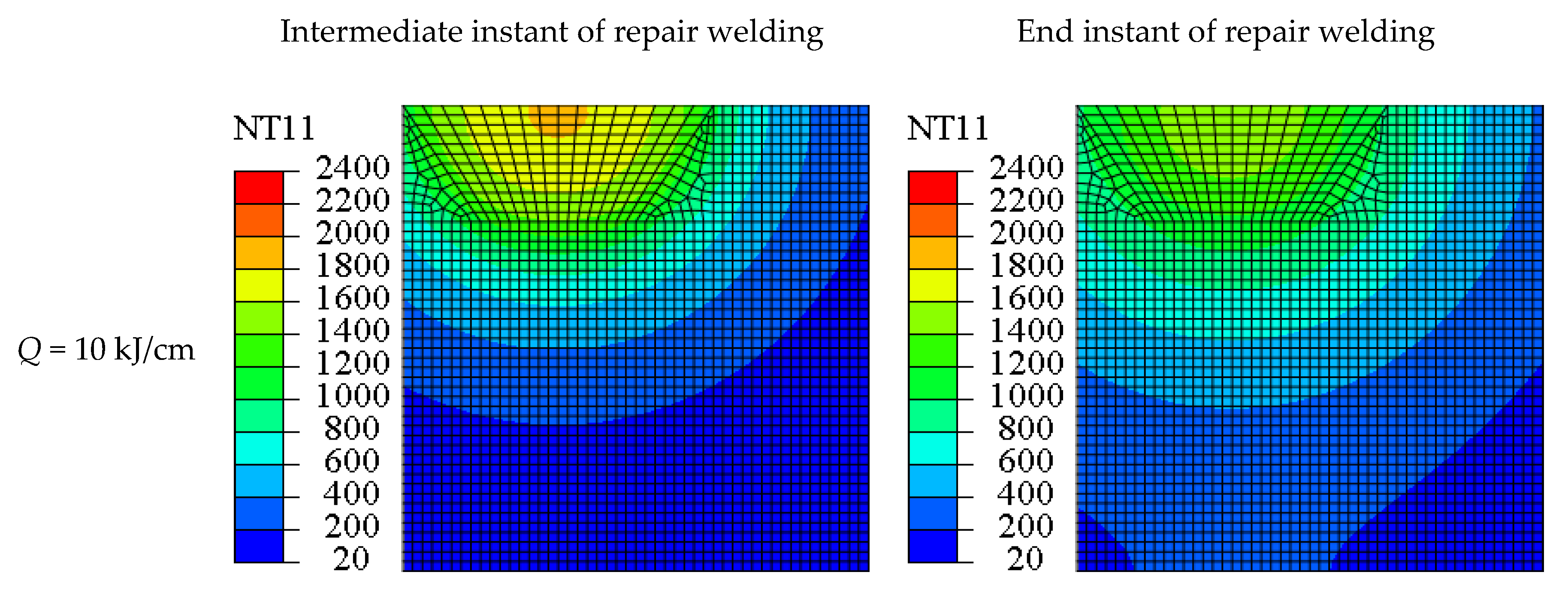
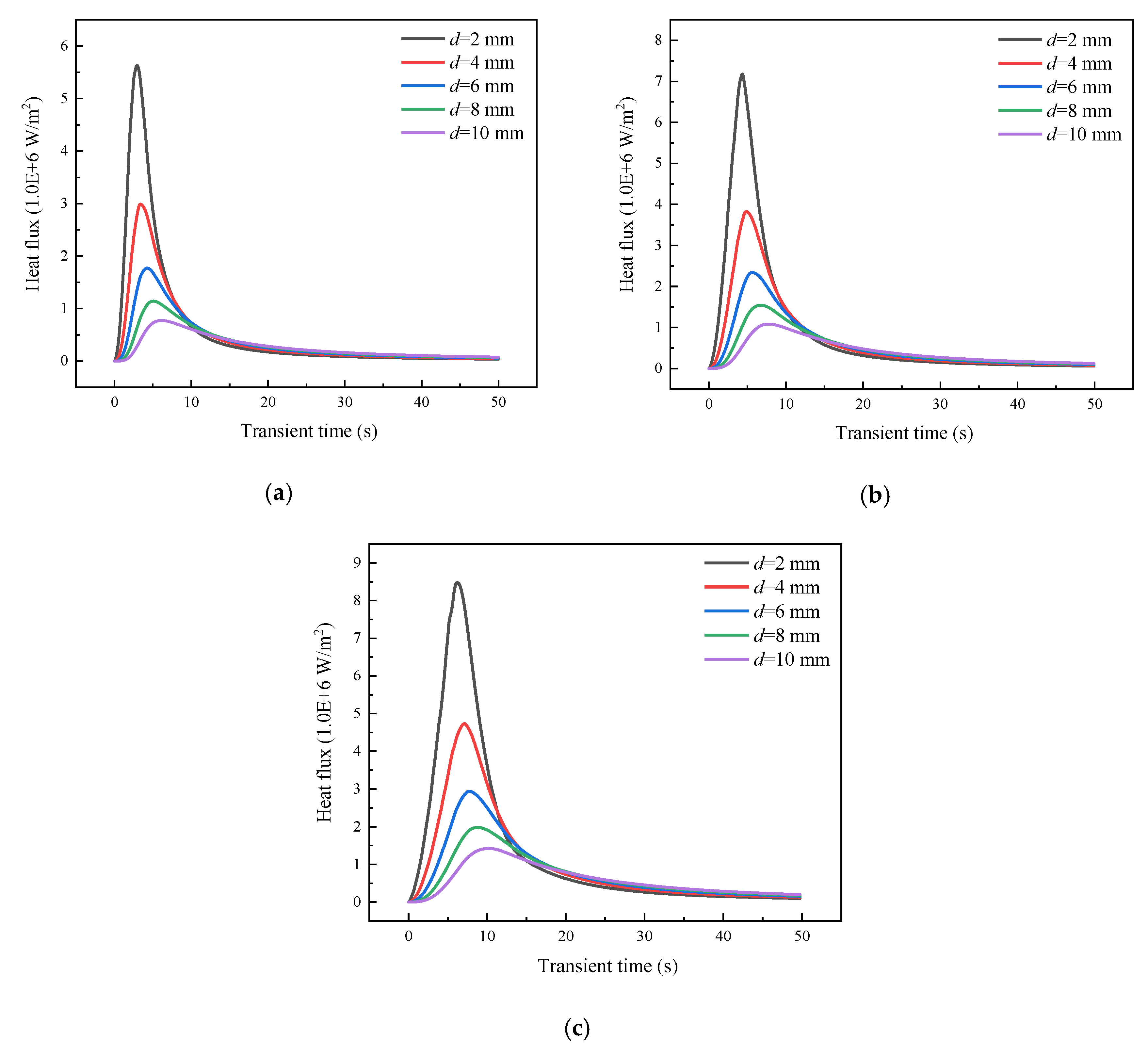
4.1. Thermal Analysis

The transient temperature contours at the intermediate instant and the end instant of repair welding for different linear energy are shown in Figure 16. The variation of linear energy has a significant influence on the temperature profile of the welding seam and HAZ. With the increase of linear energy, the peak temperature at the intermediate instant of repair welding increases. The peak temperature is 1819 °C for the linear energy of 10 kJ/cm, 2088 °C for the linear energy of 16 kJ/cm and 2320 °C for the linear energy of 25 kJ/cm. This is because higher linear energy involves longer loading times, thus more thermal energy is poured into the bulk metal during repair welding. After the intermediate instant of repair welding, due to the fact that the heat source starts to depart from the cross section, the heat generation rate decreases continuously. At the end instant of repair welding, the peak temperature for different linear energy has no obvious difference, all are around 1500 °C. In addition, with the increase of repair welding linear energy, the range of the HAZ expands. The higher linear energy brings higher overall temperature of the HAZ and poorer fracture properties.

Figure 17 shows the temperature distribution at a depth of 0.5 mm in the HAZ at the end instant of repair welding for different linear energy. The overall temperature in the HAZ increases with the increment of linear energy. The peak temperature of the HAZ is 961 °C for the linear energy of 10 kJ/cm, 1130 °C for the linear energy of 16 kJ/cm and 1258 °C for the linear energy of 25 kJ/cm. The temperature distribution of the HAZ is gentler for high linear energy.

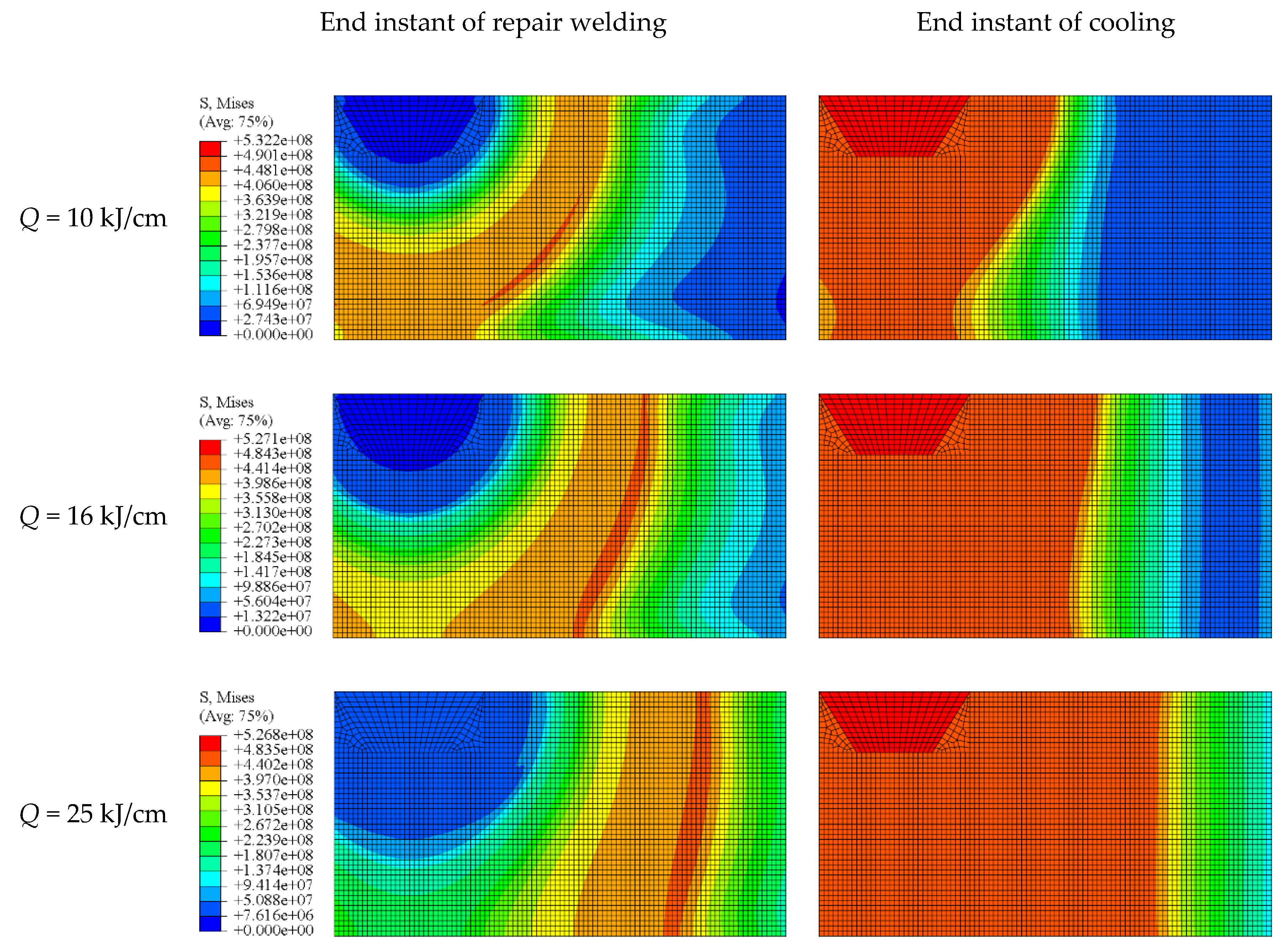
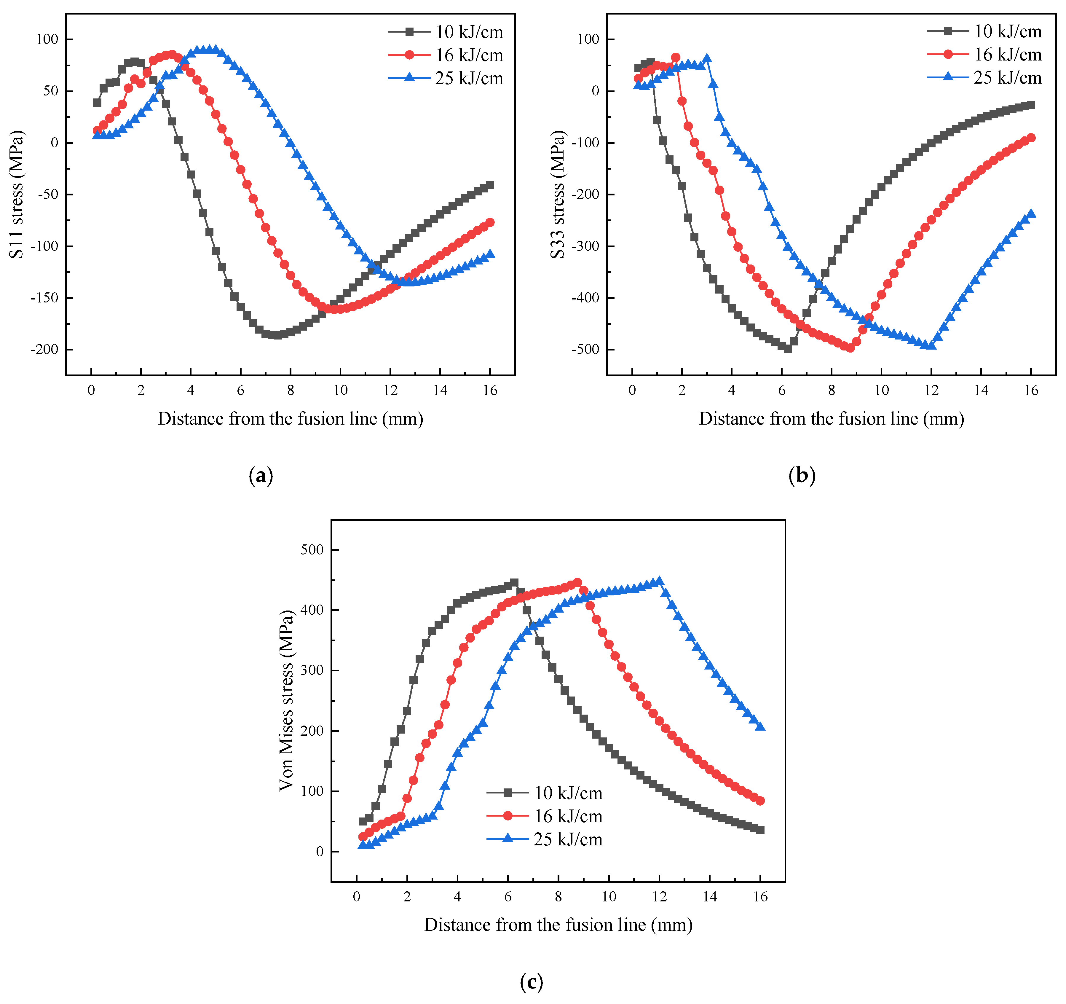
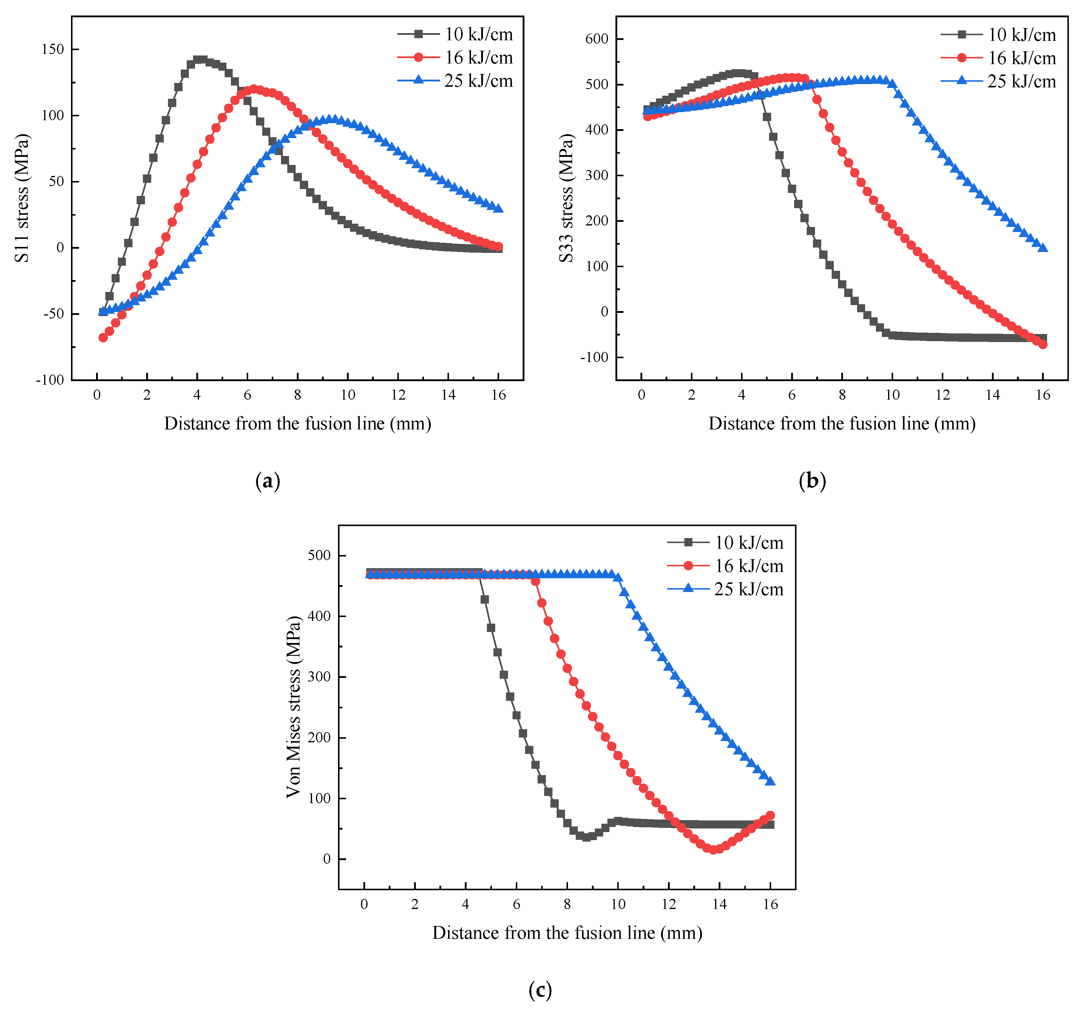
4.2. Mechanical Analysis

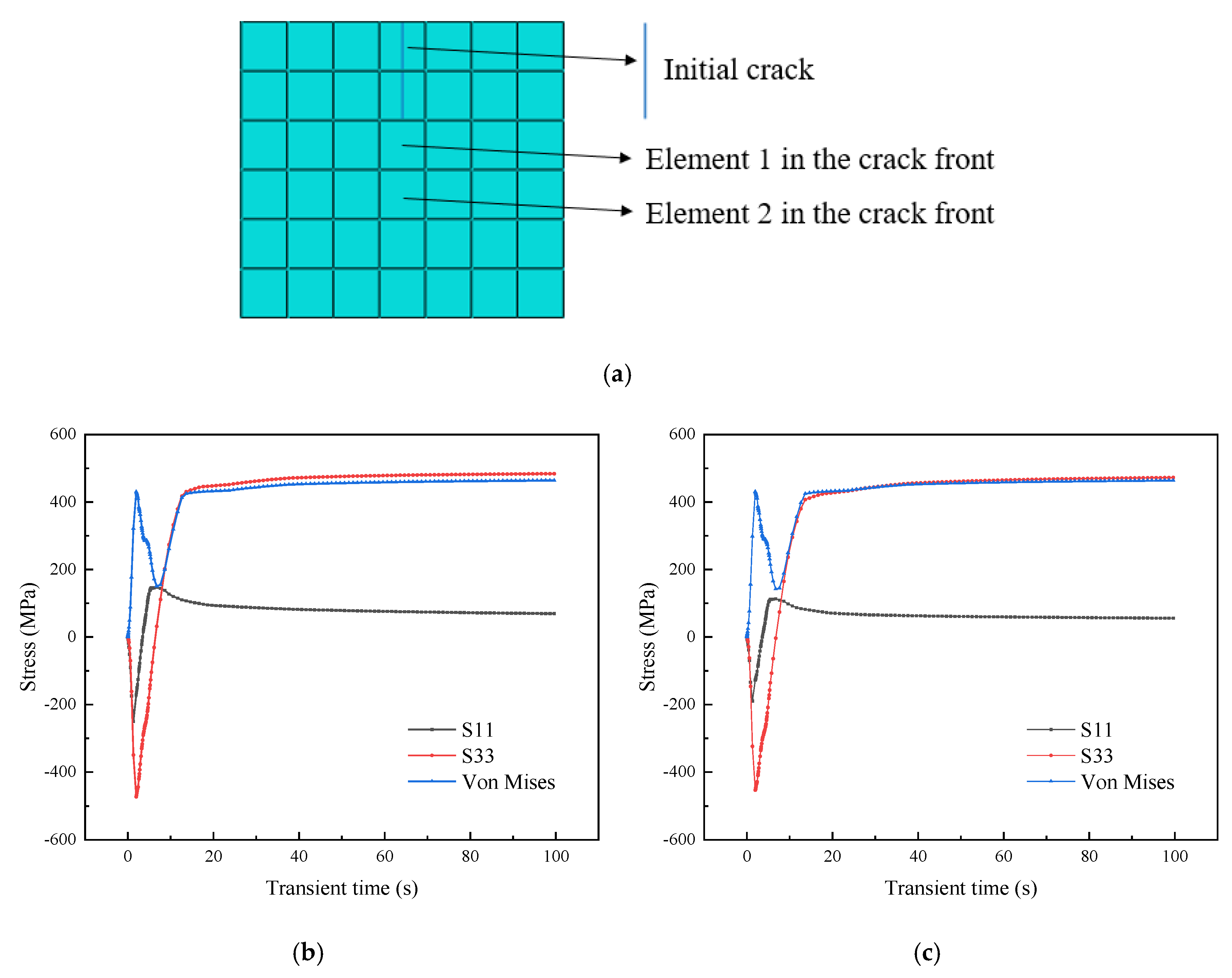
The calculated temperature field loads are used as the predefined field of stress calculation to perform the mechanical analysis. In Figure 18, the contours of the Von Mises stress field are shown at the end instant of repair welding and the end instant of cooling (the transient time at which the weld repaired component is cooled to the ambient temperature) for different linear energy. With the increase of linear energy, the range of high stress area in the HAZ at both the end instant of repair welding and the end instant of cooling expands. For different linear energy, the peak Von Mises stress in the HAZ at the end instant of repair welding and the end instant of cooling is similar. The peak Von Mises stress at the end instant of repair welding is about 445 MPa, and the peak Von Mises stress at the end instant of cooling is about 480 MPa. At the end instant of cooling, the peak Von Mises stress of the repair welding seam is greater than that of the HAZ. This is because of the different material properties considered between the weld metal and the base metal.

The S11, S33 and Von Mises stresses at a depth of 0.5 mm in the HAZ at the end instant of repair welding for different linear energy are shown in Figure 19. With the increase of linear energy, the range of high stress area of S11, S33 and Von Mises expands and moves towards the direction far away from the fusion line. The peak S33 stress and Von Mises stress has little change with the increase of linear energy, while the peak S11 stress increases slightly with the increment of linear energy. The S11 stress and S33 stress are tensile stress near the fusion line and compressive stress far away from the fusion line.

Figure 20 shows the S11, S33 and Von Mises stress distribution at a depth of 0.5 mm in the HAZ at the end instant of cooling for different linear energy. Both the S33 stress and Von Mises stress have similar peaks for different linear energy. The peak S33 stress is about 525 MPa, and the peak Von Mises stress is about 480 MPa. In the cooling process, the S11 stress near the fusion line in the HAZ changes from tensile stress to compressive stress, and the S11 stress far away from the fusion line changes from compressive stress to tensile stress. Almost all the S33 stress in the HAZ changes from compressive stress to tensile stress, and the peaks change from −500 MPa to +525 MPa, which is caused by the shrinkage of welding seam during cooling. The remarkable tensile stress may lead to the propagation of initial cracks in the HAZ. Moreover, with the increase of linear energy, the range of the high stress area in the HAZ expands. The range of the high stress area in the HAZ is 4 mm for the linear energy of 10 kJ/cm, 6 mm for the linear energy of 16 kJ/cm and 10 mm for the linear energy of 25 kJ/cm.

4.3. XFEM Analysis

Under repair welding thermal shock, the welding seam and HAZ deform plastically, so the fracture mode is elastoplastic fracture. The whole fracture process has strong nonlinearity, including not only the nonlinearity of material properties, but also the geometric nonlinearity consisting of large thermal deformation and crack propagation.

The crack at the position of d = 2 mm under the repair welding linear energy of 10 kJ/cm is selected to analyze and the simulated crack propagation paths are shown in Figure 21. It is noteworthy that the crack propagation occurs during the cooling process, which is in agreement with the mechanical analysis. The crack propagation direction is almost perpendicular to the surface due to the control of MPS criterion and there is a certain tendency for the crack to deflect to the welding seam during the propagation process. A total of two elements are extended and the extracted crack propagation length is 0.52 mm. Figure 21a shows the MPS contours for the crack zone at different transient times. t = 3.96 s is the end instant of repair welding and the start instant of cooling. At the start instant of cooling, the MPS around the crack tip is lower than the allowable MPS at the corresponding temperature according to the damage initiation criterion, so the crack does not propagate. With the cooling process going on, the tensile stress increases continuously, which leads to the increment of the MPS around the crack tip. At t = 4.43 s, the crack damage initiation condition is reached, and the new crack surface begins to form. After the formation of the new crack surface, the stress concentration around the crack tip is released and the MPS decreases. A new driving force is required to promote the further crack propagation. At t = 5.22 s, the new driving force makes the crack extend further.

Figure 21b shows the status of the enriched element (STATUSXFEM) for the crack zone at different transient times. The variable STATUSXFEM represents the damage degree of the crack, ranging from 0 to 1.0. A value of 0 means that the material has no damage. A value of 1.0 means that the crack is fully opened and the cohesive traction between the crack surfaces is zero. When the value is greater than 0 and less than 1.0, it means that the cohesive crack has already extended and needs extra driving force to fully open. Although the new cracks are not fully opened, in the complex service environment, the cohesive cracks containing damage are likely to open completely after being driven by the extra driving force, which threatens the structural integrity of weld repaired components.

According to the crack propagation paths in Figure 21, two elements in the initial crack front are selected to analyze. The transient S11, S33 and Von Mises stresses of the elements under repair welding thermal shock are shown in Figure 22. The first 3.96 s of transient time is the repair welding process. In this process, the HAZ is compressed due to the outward expansion of the welding seam. The S11 and S33 stresses are compressive stress, and the value of compressive stress increases with the promoting of repair welding. After repair welding, the welding seam begins to cool and shrink, which results in the tensile stress in the HAZ. The S11 and S33 stress changes from compressive stress to tensile stress in the early stage of cooling and the crack propagation occurs in this stage.

In order to investigate the influence of repair welding thermal shock on the cracks at different distances from the fusion line for three different linear energy values, the initial cracks with a size of 0.5 mm perpendicular to the surface were prefabricated at the positions where the distances from the fusion line were 2 mm, 4 mm, 6 mm, 8 mm and 10 mm, respectively. Figure 23 shows the crack propagation predicted by XFEM at different positions for three different linear energy values. All the crack propagation occurs in the early stage of cooling. For cracks at the same location, with the increase of linear energy, the crack propagation length and the number of damaged elements increase. This is because the higher linear energy brings the higher temperature of the HAZ, which leads to poorer crack resistance. The longest crack propagation appears at the position of d = 2 mm under the linear energy of 25 kJ/cm. The extracted crack propagation length is 1.1 mm, which is almost twice of the initial crack length. In this case, the fully opened crack propagation has occurred, and the crack is likely to develop into the macrocrack, even penetrate through the whole wall thickness. For the same linear energy, the crack propagation length decreases with the increment of distance from the fusion line. Both the cracks with d > 6 mm for the linear energy of 10 kJ/cm and the cracks with d > 8 mm for the linear energy of 16 kJ/cm do not propagate. The reason is that the lower the linear energy is, the smaller the scope of the HAZ is. Once the crack is far away from the fusion line, the driving force is not enough to promote the crack propagation. It should be noted that the area where cracks propagate is the high stress area where the peak stress is located. Almost all the directions of crack propagation are perpendicular to the surface and tend to deflect to the welding seam, which may be related to the high stress in the welding seam.

Since the crack resistance of materials is related to temperature, the temperature at the crack tip is one of the key factors affecting crack propagation. On the one hand, the higher the temperature is, the poorer the crack resistance is, and the cracks are easier to extend under the same driving force. On the other hand, the larger the temperature gradient is, the greater the thermal stress is, so the driving force is sufficient for crack propagation. Figure 24 shows the thermal cycle curves at different crack tips in the HAZ for three different linear energy values. For the same linear energy, with the decrease of the distance from the fusion line, the difference of the peak temperature at the crack tip becomes larger. As a result, the closer the crack is to the fusion line, the greater the temperature gradient and temperature change around the crack tip, the greater the driving force and the longer the crack propagation length. For the same crack tip, the peak temperature increases with the increment of linear energy. Therefore, the greater the linear energy is, the poorer the crack resistance of materials in the HAZ is. In the early stage of cooling, the temperature value in the HAZ is higher and the temperature difference in the HAZ is larger, so crack propagation occurs in the early stage of cooling. With the cooling process going on, the temperature at the crack tip at different positions gradually tends to become consistent.

The distribution of heat flux through the crack surfaces with the transient time is shown in Figure 25. The distribution of heat flux is similar to the thermal cycle curves at crack tips, which indicates that the temperature at crack tips is proportional to the thermal energy density through the crack surfaces. For the same crack surface, the peak heat flux increases with the increment of linear energy. For the same linear energy, in repair welding process and early stage of cooling, the closer the crack surface is to the fusion line, the greater the heat flux gradient is and the greater the heat flux change is.

5. Conclusions

In this study, the XFEM based on a cohesive crack model is used to establish the repair welding model of P91 steel welded joint containing initial cracks. The MPS criterion and energy method are used to define the damage initiation and damage evolution, respectively. Considering the temperature-dependent material physical properties and fracture properties, the effect of repair welding thermal shock on the crack propagation behavior in the HAZ is simulated. The influence of different repair welding linear energy and different crack positions on the cracking features is analyzed. The main conclusions are as follows:

(1)

With the increase of linear energy, the range of the HAZ expands and the overall temperature of the HAZ rises. With the increase of linear energy, the range of S11, S33 and Von Mises high stress area expands.

(2)

In the repair welding and cooling process, the material in the HAZ undergoes a change from compressed state to tensioned state due to the expansion and shrinkage of the welding seam. It is the direct cause of crack propagation in the HAZ.

(3)

Crack propagation occurs in the early stage of cooling. The crack propagation direction is roughly perpendicular to the upper surface and has a tendency to deflect to the welding seam.

(4)

For cracks at the same position, with the increase of linear energy, the crack propagation length increases. For the same linear energy, with the distance from the fusion line increases, the crack propagation length decreases.

(5)

After a certain distance from the fusion line, the cracks in the HAZ do not extend. This distance is the critical distance for the crack propagation. With the increase of linear energy, the critical distance of crack propagation increases. The critical distance of crack propagation is consistent with the high stress area after repair welding. Therefore, for repair welding, low linear energy is preferred to constrain the cracking behavior in the HAZ.

References

1. Viswanathan, R.; Coleman, K.; Rao, U. Materials for ultra-supercritical coal-fired power plant boilers. Int. J. Pres. Vessel Pip. 2006, 83, 778–783. [Google Scholar] [CrossRef]
2. Klueh, R.L. Elevated temperature ferritic and martensitic steels and their application to future nuclear reactors. Int. Mater. Rev. 2005, 50, 287–310. [Google Scholar] [CrossRef] [Green Version]
3. Chu, Q.L.; Zhang, M.; Li, J.H.; Chen, Y.N.; Luo, H.L.; Wang, Q. Failure analysis of a steam pipe weld used in power generation plant. Eng. Fail. Anal. 2014, 44, 363–370. [Google Scholar] [CrossRef]
4. Hu, Z.X.; Zhao, J.P. Effects of martensitic transformation on residual stress of P91 welded joint. Mater. Res. Express 2018, 5, 096528. [Google Scholar] [CrossRef]
5. Abson, D.J.; Rothwell, J.S. Review of type IV cracking of weldments in 9–12%Cr creep strength enhanced ferritic steels. Int. Mater. Rev. 2013, 58, 437–473. [Google Scholar] [CrossRef]
6. Viswanathan, R.; Gandy, D. Weld Repair of Aged Cr-Mo Steel Piping—A Review of Literature. J. Press. Vessel Technol. ASME 2000, 122, 76–85. [Google Scholar] [CrossRef]
7. Parker, J.D.; Siefert, J.A. Weld repair of Grade 91 piping and components in power generation applications, creep performance of repair welds. Mater. High. Temp. 2016, 33, 58–67. [Google Scholar] [CrossRef]
8. Weglowski, M. Determination of GTA and GMA welding arc temperatures. Weld. Int. 2005, 19, 186–192. [Google Scholar] [CrossRef]
9. Alvarez, P.; Vázquez, L.; Ruiz, N.; Rodríguez, P.; Magaña, A.; Niklas, A.; Santos, F. Comparison of hot cracking susceptibility of TIG and laser beam welded alloy 718 by varestraint testing. Metals 2019, 9, 985. [Google Scholar] [CrossRef] [Green Version]
10. Chelladurai, A.M.; Gopal, K.A.; Murugan, S.; Albert, S.K.; Venugopal, S.; Jayakumar, T. Effect of energy transfer modes on solidification cracking in pulsed laser welding. Sci. Technol. Weld. Join. 2015, 20, 578–584. [Google Scholar] [CrossRef]
11. Hosseini, S.A.; Abdollah-zadeh, A.; Naffakh-Moosavy, H.; Mehri, A. Elimination of hot cracking in the electron beam welding of AA2024-T351 by controlling the welding speed and heat input. J. Manuf. Process. 2019, 46, 147–158. [Google Scholar] [CrossRef]
12. Coniglio, N.; Cross, C.E. Mechanisms for solidification crack initiation and growth in aluminum welding. Metall. Mater. Trans. A 2009, 40, 2718–2728. [Google Scholar] [CrossRef]
13. Wei, Y.H.; Liu, R.P.; Dong, Z.J. Software package for simulation and prediction of welding solidification cracks. Sci. Technol. Weld. Join. 2003, 8, 325–333. [Google Scholar] [CrossRef]
14. Bordreuil, C.; Niel, A. Modelling of hot cracking in welding with a cellular automaton combined with an intergranular fluid flow model. Comp. Mater. Sci. 2014, 82, 442–450. [Google Scholar] [CrossRef] [Green Version]
15. Agarwal, G.; Kumar, A.; Richardson, I.M.; Hermans, M.J.M. Evaluation of solidification cracking susceptibility during laser welding in advanced high strength automotive steels. Mater. Des. 2019, 183, 108104. [Google Scholar] [CrossRef]
16. Jiang, W.C.; Liu, Z.B.; Gong, J.M.; Tu, S.T. Numerical simulation to study the effect of repair width on residual stresses of a stainless steel clad plate. Int. J. Pres. Ves. Pip. 2010, 87, 457–463. [Google Scholar] [CrossRef]
17. Hyde, T.H.; Saber, M.; Sun, W. Creep crack growth data and prediction for a P91 weld at 650 °C. Int. J. Pres. Ves. Pip. 2010, 87, 721–729. [Google Scholar] [CrossRef]
18. Pandey, C.; Saini, N.; Mahapatra, M.M.; Kumar, P. Hydrogen induced cold cracking of creep resistant ferritic P91 steel for different diffusible hydrogen levels in deposited metal. Int. J. Hydrogen. Energy 2016, 41, 17695–17712. [Google Scholar] [CrossRef]
19. Zhang, Y.J.; Yang, K.; Zhao, J.P. Experimental research and numerical simulation of weld repair with high energy spark deposition method. Metals 2020, 10, 980. [Google Scholar] [CrossRef]
20. He, K.F.; Yang, Q.; Xiao, D.M.; Li, X.J. Analysis of thermo-elastic fracture problem during aluminium alloy MIG welding using the extended finite element method. Appl. Sci. 2017, 7, 69. [Google Scholar] [CrossRef] [Green Version]
21. Li, H.; Li, J.S.; Yuan, H. A review of the extended finite element method on macrocrack and microcrack growth simulations. Theor. Appl. Fract. Mech. 2018, 97, 236–249. [Google Scholar] [CrossRef]
22. Belytschko, T.; Black, T. Elastic crack growth in finite elements with minimal remeshing. Int. J. Numer. Meth. Eng. 1999, 45, 601–620. [Google Scholar] [CrossRef]
23. Moës, N.; Dolbow, J.; Belytschko, T. A finite element method for crack growth without remeshing. Int. J. Numer. Meth. Eng. 1999, 46, 131–150. [Google Scholar] [CrossRef]
24. Daux, C.; Moës, N.; Dolbow, J.; Sukumar, N.; Belytschko, T. Arbitrary branched and intersecting cracks with the extended finite element method. Int. J. Numer. Meth. Eng. 2000, 48, 1741–1760. [Google Scholar] [CrossRef]
25. Chessa, J.; Wang, H.W.; Belytschko, T. On the construction of blending elements for local partition of unity enriched finite elements. Int. J. Numer. Meth. Eng. 2003, 57, 1015–1038. [Google Scholar] [CrossRef]
26. Stolarska, M.; Chopp, D.L.; Moës, N.; Belytschko, T. Modelling crack growth by level sets in the extended finite element method. Int. J. Numer. Meth. Eng. 2001, 51, 943–960. [Google Scholar] [CrossRef]
27. Song, J.-H.; Areias, P.M.A.; Belytschko, T. A method for dynamic crack and shear band propagation with phantom nodes. Int. J. Numer. Meth. Eng. 2006, 67, 868–893. [Google Scholar] [CrossRef]
28. Yang, J.P.; Guo, J.; Qiao, Y.X. DL/T 869-2012 The Code of Welding for Power Plant; China Electric Power Press: Beijing, China, 2012. (In Chinese) [Google Scholar]
29. Yaghi, A.H.; Hyde, T.H.; Becker, A.A.; Williams, J.A.; Sun, W. Residual stress simulation in welded sections of P91 pipes. J. Mater. Process. Tech. 2005, 167, 480–487. [Google Scholar] [CrossRef]
30. Arora, H.; Singh, R.; Brar, G.S. Thermal and structural modelling of arc welding processes: A literature review. Meas. Control. 2019, 52, 955–969. [Google Scholar] [CrossRef]
31. Zhang, W.Y. Principle and Technology of Metal; Fusion Welding; China Machine Press: Beijing, China, 1980. (In Chinese) [Google Scholar]
32. Zhang, J.X.; Liu, C. Finite Element Calculation of Welding Stress and Deformation and Its Engineering Application; Science Press: Beijing, China, 2015. (In Chinese) [Google Scholar]
33. Asferg, J.L.; Poulsen, P.N.; Nielsen, L.O. A direct XFEM formulation for modeling of cohesive crack growth in concrete. Comput. Concr. 2007, 4, 83–100. [Google Scholar] [CrossRef]
34. Benzeggagh, M.L.; Kenane, M. Measurement of mixed-mode delamination fracture toughness of unidirectional glass/epoxy composites with mixed-mode bending apparatus. Compos. Sci. Technol. 1996, 56, 439–449. [Google Scholar] [CrossRef]
35. Pan, J.Z. Practical Manual for Pressure Vessel Materials—Carbon Steel and Alloy Steel; Chemical Industry Press: Beijing, China, 2000. (In Chinese) [Google Scholar]
36. Dutt, B.S.; Babu, M.N.; Shanthi, G.; Moitra, A.; Sasikala, G. Investigation on fracture behavior of Grade 91 steel at 300–550 °C. J. Mater. Eng. Perform. 2018, 27, 6577–6584. [Google Scholar] [CrossRef]
37. ASME. ASME Boiler & Pressure Vessel Code, Section II, Part A; American Society of Mechanical Engineers: New York, NY, USA, 2019. [Google Scholar]
38. ASME. ASME Boiler & Pressure Vessel Code, Section II, Part C; American Society of Mechanical Engineers: New York, NY, USA, 2019. [Google Scholar]
39. Chen, H.N.; Li, R.F.; Chen, J. GB/T 24179-2009 Metallic Materials-Residual Stress Determination—The Indentation Strain-Gage Method; China Standard Press: Beijing, China, 2009. (In Chinese) [Google Scholar]
Figure 1. Crack classification of Cr-Mo steel welded joint, reproduced from [5], with permission from International Materials Reviews, 2020.
Metals 10 01285 g001
Figure 2. Cut element and blending element in the extended finite element method (XFEM).
Metals 10 01285 g002
Figure 3. Schematic drawing of the model geometry. (unit: mm).
Metals 10 01285 g003
Figure 4. The location of the cross section for analysis. (unit: mm).
Metals 10 01285 g004
Figure 5. Finite element (FE) model and meshing.
Metals 10 01285 g005
Figure 6. Temperature-dependent thermal physical properties and mechanical properties, for base metal and weld metal, used in the FE simulation, data from [29].
Metals 10 01285 g006
Figure 7. Action volume of the heat source.
Metals 10 01285 g007
Figure 8. Time distribution of heat generation rate under different linear energy.
Metals 10 01285 g008
Figure 9. The traction-separation law.
Metals 10 01285 g009
Figure 10. Temperature-dependent fracture properties for P91 steel, used in the FE simulation, data from [35,36].
Metals 10 01285 g010
Figure 11. Precrack definition: (a) the physical model with a precrack; (b) the XFEM model with a precrack.
Metals 10 01285 g011
Figure 12. Morphology of specimens: (a) after initial welding; (b) after repair welding; (c) morphology of welding layers.
Metals 10 01285 g012
Figure 13. Position of measuring points for specimens (unit: mm): (a) after initial welding; (b) after repair welding.
Metals 10 01285 g013
Figure 14. The measurement of residual stress: (a) residual stress measurement system; (b) residual stress on-site measuring.
Metals 10 01285 g014
Figure 15. Comparison of the residual stress obtained from FE simulations and experiments: (a) S11 stress after initial welding; (b) S33 stress after initial welding; (c) S11 stress after repair welding; (d) S33 stress after repair welding.
Metals 10 01285 g015aMetals 10 01285 g015b
Figure 16. Temperature contours at the intermediate instant and the end instant of repair welding for different linear energy.
Metals 10 01285 g016aMetals 10 01285 g016b
Figure 17. Temperature distribution at a depth of 0.5 mm in the heat affected zone (HAZ) at the end instant of repair welding for different linear energy.
Metals 10 01285 g017
Figure 18. Stress contours at the end instant of repair welding and the end instant of cooling for different linear energy.
Metals 10 01285 g018
Figure 19. Stress distribution at a depth of 0.5 mm in the HAZ at the end instant of repair welding for different linear energy: (a) S11 stress in the HAZ; (b) S33 stress in the HAZ; (c) Von Mises stress in the HAZ.
Metals 10 01285 g019
Figure 20. Stress distribution at a depth of 0.5 mm in the HAZ at the end instant of cooling for different linear energy: (a) S11 stress in the HAZ; (b) S33 stress in the HAZ; (c) Von Mises stress in the HAZ.
Metals 10 01285 g020
Figure 21. Crack propagation paths at different transient times (d = 2 mm, Q = 10 kJ/cm): (a) maximum principal stress (MPS) contours; (b) status of the enriched element (STATUSXFEM).
Metals 10 01285 g021
Figure 22. Transient stress curves of the elements in the crack front: (a) initial crack and elements in the crack front; (b) element 1; (c) element 2.
Metals 10 01285 g022
Figure 23. Crack propagation predicted by XFEM at different positions for three different linear energy values.
Metals 10 01285 g023
Figure 24. Thermal cycle curves at crack tips in the HAZ for three different linear energy values: (a) Q = 10 kJ/cm; (b) Q = 16 kJ/cm; (c) Q = 25 kJ/cm.
Metals 10 01285 g024
Figure 25. Heat flux distribution through crack surfaces in the HAZ for three different linear energy values: (a) Q = 10 kJ/cm; (b) Q = 16 kJ/cm; (c) Q = 25 kJ/cm.
Metals 10 01285 g025