Hot Metal Temperature Forecasting at Steel Plant Using Multivariate Adaptive Regression Splines


Abstract
1. Introduction
2. Materials and Methods
2.1. Explanatory Variables
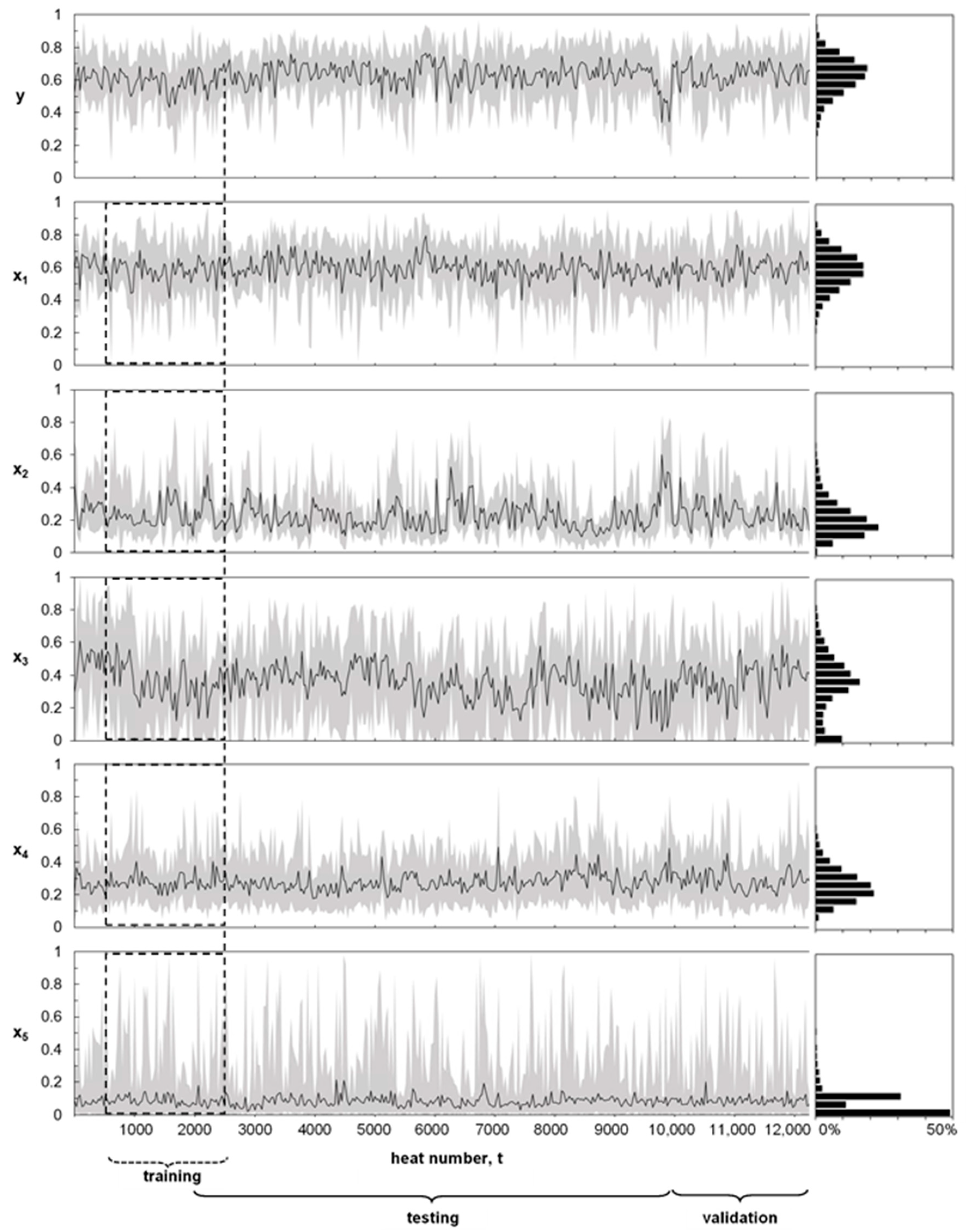
2.2. Process Dataset
2.3. Multivariate Adaptive Regression Splines with Moving Training Window
2.3.1. Forward Phase
2.3.2. Backward Phase
2.3.3. Model Hyperparameters
3. Results
3.1. Computation
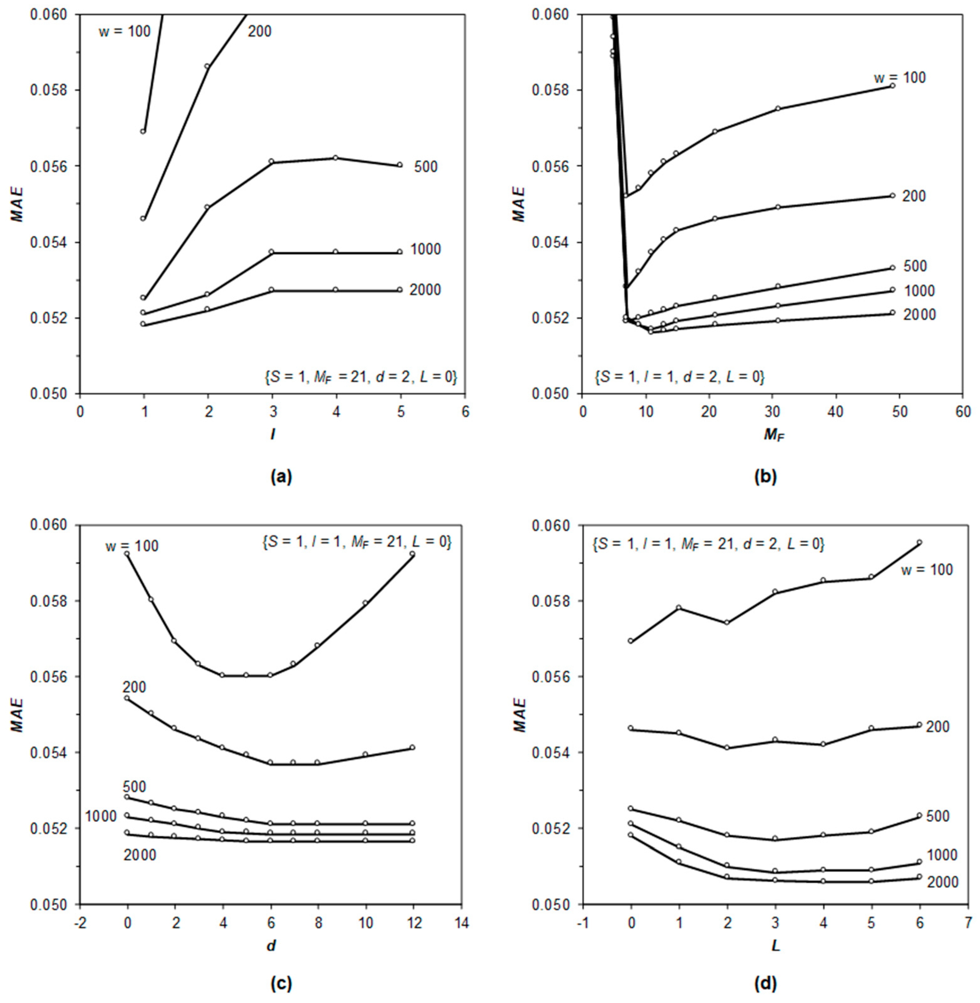
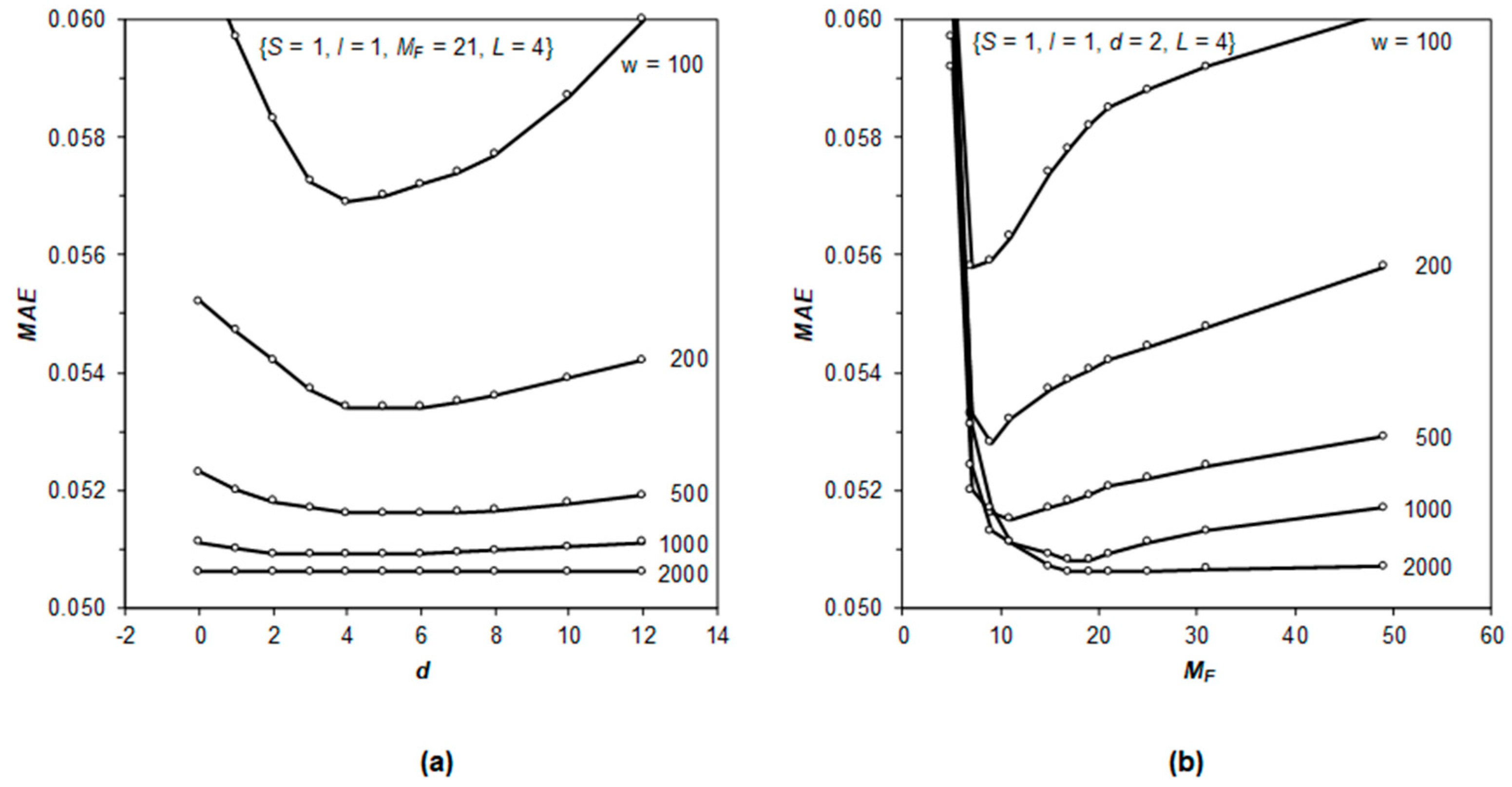
3.2. Study of Hyperparameters
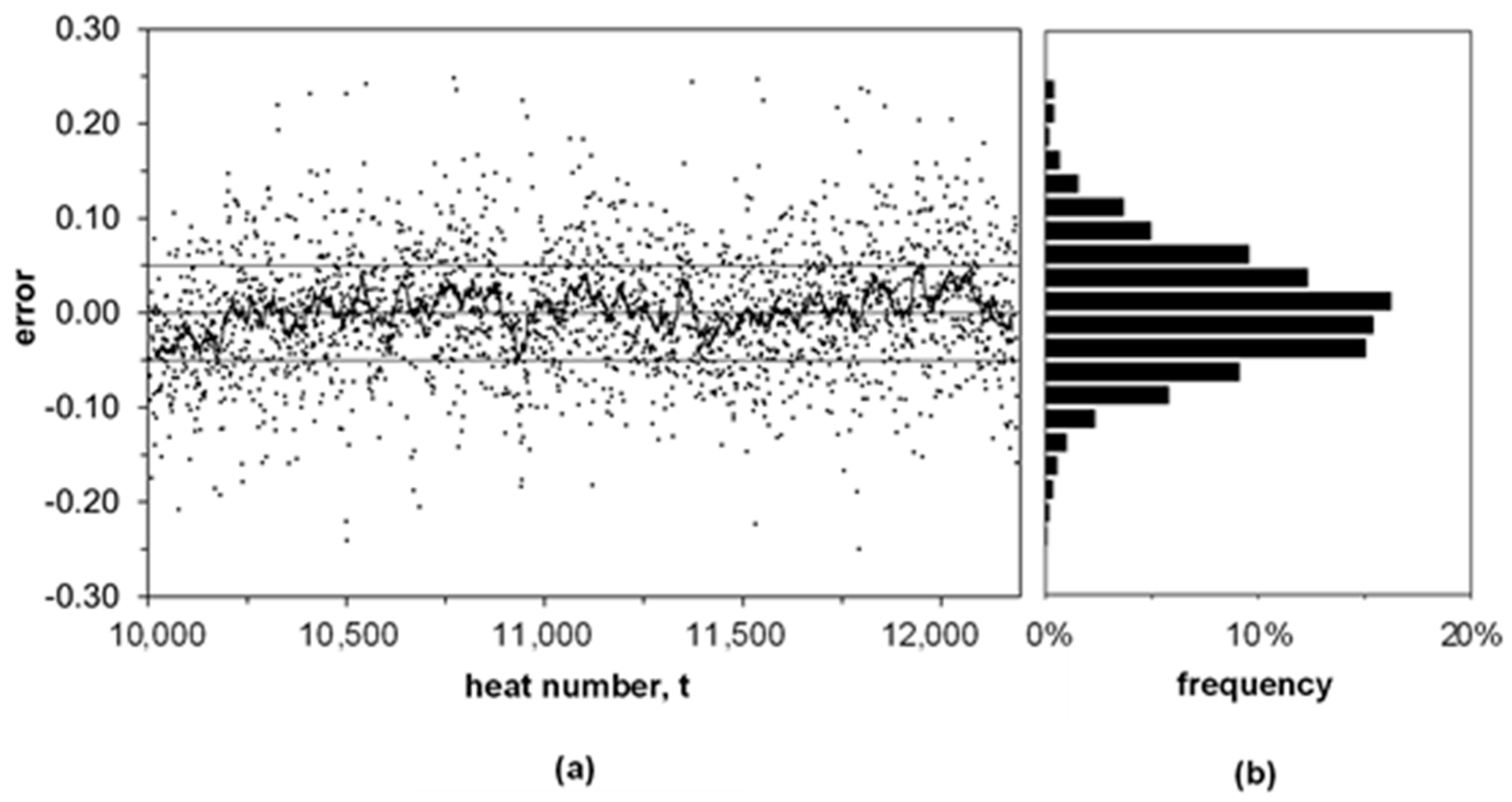
3.3. Model Validation
4. Discussion
5. Conclusions
Supplementary Materials
Author Contributions
Funding
Acknowledgments
Conflicts of Interest
References
- McLean, A. The science and technology of steelmaking—Measurements, models, and manufacturing. Metall. Mater. Trans. B 2006, 37, 319–332. [Google Scholar] [CrossRef]
- Ghosh, A.; Chatterjee, A. Iron Making and Steelmaking: Theory and Practice; PHI Learning Pvt. Ltd.: New Delhi, India, 2008. [Google Scholar]
- Miller, T.W.; Jimenez, J.; Sharan, A.; Goldstein, D.A. Oxygen Steelmaking Processes. In The Making, Shaping, and Treating of Steel, 11th ed.; Fruehan, R.J., Ed.; The AISE Steel Foundation: Pittsburgh, PA, USA, 1998; pp. 475–524. [Google Scholar]
- Williams, R.V. Control of oxygen steelmaking. In Control and Analysis in Iron and Steelmaking, 1st ed.; Butterworth Scientific Ltd.: London, UK, 1983; pp. 147–176. [Google Scholar]
- Jiménez, J.; Mochón, J.; de Ayala, J.S.; Obeso, F. Blast furnace hot metal temperature prediction through neural networks-based models. ISIJ Int. 2004, 44, 573–580. [Google Scholar] [CrossRef]
- Martín, R.D.; Obeso, F.; Mochón, J.; Barea, R.; Jiménez, J. Hot metal temperature prediction in blast furnace using advanced model based on fuzzy logic tools. Ironmak. Steelmak. 2007, 34, 241–247. [Google Scholar] [CrossRef]
- Sugiura, M.; Shinotake, A.; Nakashima, M.; Omoto, N. Simultaneous Measurements of Temperature and Iron–Slag Ratio at Taphole of Blast Furnace. Int. J. Thermophys. 2014, 35, 1320–1329. [Google Scholar] [CrossRef]
- Jiang, Z.H.; Pan, D.; Gui, W.H.; Xie, Y.F.; Yang, C.H. Temperature measurement of molten iron in taphole of blast furnace combined temperature drop model with heat transfer model. Ironmak. Steelmak. 2018, 45, 230–238. [Google Scholar] [CrossRef]
- Pan, D.; Jiang, Z.; Chen, Z.; Gui, W.; Xie, Y.; Yang, C. Temperature Measurement Method for Blast Furnace Molten Iron Based on Infrared Thermography and Temperature Reduction Model. Sensors 2018, 18, 3792. [Google Scholar] [CrossRef]
- Pan, D.; Jiang, Z.; Chen, Z.; Gui, W.; Xie, Y.; Yang, C. Temperature Measurement and Compensation Method of Blast Furnace Molten Iron Based on Infrared Computer Vision. IEEE Trans. Instrum. Meas. 2018, 1–13. [Google Scholar] [CrossRef]
- Jin, S.; Harmuth, H.; Gruber, D.; Buhr, A.; Sinnema, S.; Rebouillat, L. Thermomechanical modelling of a torpedo car by considering working lining spalling. Ironmak. Steelmak. 2018, 1–5. [Google Scholar] [CrossRef]
- Frechette, M.; Chen, E. Thermal insulation of torpedo cars. In Proceedings of the Association for Iron and Steel Technology (Aistech) Conference Proceedings, Charlotte, NC, USA, 9–12 May 2005. [Google Scholar]
- Nabeshima, Y.; Taoka, K.; Yamada, S. Hot metal dephosphorization treatment in torpedo car. Kawasaki Steel Tech. Rep. 1991, 24, 25–31. [Google Scholar]
- Niedringhaus, J.C.; Blattner, J.L.; Engel, R. Armco’s Experimental 184 Mile Hot Metal Shipment. In Proceedings of the 47th Ironmaking Conference, Toronto, ON, Canada, 17–20 April 1988. [Google Scholar]
- Goldwaser, A.; Schutt, A. Optimal torpedo scheduling. J. Artif. Intell. Res. 2018, 63, 955–986. [Google Scholar] [CrossRef]
- Wang, G.; Tang, L. A column generation for locomotive scheduling problem in molten iron transportation. In Proceedings of the 2007 IEEE International Conference on Automation and Logistics, Jinan, China, 18–21 August 2007. [Google Scholar]
- He, F.; He, D.F.; Xu, A.J.; Wang, H.B.; Tian, N.Y. Hybrid model of molten steel temperature prediction based on ladle heat status and artificial neural network. J. Iron Steel Res. Int. 2014, 21, 181–190. [Google Scholar] [CrossRef]
- Du, T.; Cai, J.J.; Li, Y.J.; Wang, J.J. Analysis of Hot Metal Temperature Drop and Energy-Saving Mode on Techno-Interface of BF-BOF Route. Iron Steel 2008, 43, 83–86, 91. [Google Scholar]
- Liu, S.W.; Yu, J.K.; Yan, Z.G.; Liu, T. Factors and control methods of the heat loss of torpedo-ladle. J. Mater. Metall. 2010, 9, 159–163. [Google Scholar]
- Wu, M.; Zhang, Y.; Yang, S.; Xiang, S.; Liu, T.; Sun, G. Analysis of hot metal temperature drop in torpedo car. Iron Steel 2002, 37, 12–15. [Google Scholar]
- Díaz, J.; Fernández, F.J.; Suárez, I. Hot Metal Temperature Prediction at Basic-Lined Oxygen Furnace (BOF) Converter Using IR Thermometry and Forecasting Techniques. Energies 2019, 12, 3235. [Google Scholar] [CrossRef]
- Díaz, J.; Fernandez, F.J.; Gonzalez, A. Prediction of hot metal temperature in a BOF converter using an ANN. In Proceedings of the IRCSEEME 2018: International Research Conference on Sustainable Energy, Engineering, Materials and Environment, Mieres, Spain, 25–27 July 2018. [Google Scholar]
- Friedman, J.H. Multivariate adaptive regression splines. Ann. Stat. 1991, 19, 1–67. [Google Scholar] [CrossRef]
- Friedman, J.H.; Roosen, C.B. An Introduction to Multivariate Adaptive Regression Splines. Stat. Methods Med. Res. 1995, 4, 197–217. [Google Scholar] [CrossRef]
- Nieto, P.; Suárez, V.; Antón, J.; Bayón, R.; Blanco, J.; Fernández, A. A new predictive model of centerline segregation in continuous cast steel slabs by using multivariate adaptive regression splines approach. Materials 2015, 8, 3562–3583. [Google Scholar] [CrossRef]
- Mukhopadhyay, A.; Iqbal, A. Prediction of mechanical property of steel strips using multivariate adaptive regression splines. J. Appl. Stat. 2009, 36, 1–9. [Google Scholar] [CrossRef]
- Yu, W.H.; Yao, C.G.; Yi, X.D. A Predictive Model of Hot Rolling Flow Stress by Multivariate Adaptive Regression Spline. In Materials Science Forum; Trans Tech Publications Ltd.: Stafa-Zurich, Switzerland, 2017; Volume 898, pp. 1148–1155. [Google Scholar]
- Mehdizadeh, S.; Behmanesh, J.; Khalili, K. Comprehensive modeling of monthly mean soil temperature using multivariate adaptive regression splines and support vector machine. Theor. Appl. Climatol. 2018, 133, 911–924. [Google Scholar] [CrossRef]
- Yang, C.C.; Prasher, S.O.; Lacroix, R.; Kim, S.H. Application of multivariate adaptive regression splines (MARS) to simulate soil temperature. Trans. ASAE 2004, 47, 881. [Google Scholar] [CrossRef]
- Krzemień, A. Fire risk prevention in underground coal gasification (UCG) within active mines: Temperature forecast by means of MARS models. Energy 2019, 170, 777–790. [Google Scholar] [CrossRef]
- Kuhn, M.; Johnson, K. Nonlinear regression models. In Applied Predictive Modeling, 1st ed.; Springer: New York, NY, USA, 2010; pp. 145–151. [Google Scholar]
- Jekabsons, G. ARESLab: Adaptive Regression Splines Toolbox for Matlab/Octave. 2016. Available online: http://www.cs.rtu.lv/jekabsons/Files/ARESLab.pdf (accessed on 15 November 2019).
- Saltelli, A.; Ratto, M.; Andres, T.; Campolongo, F.; Cariboni, J.; Gatelli, D.; Tarantola, S. Global Sensitivity Analysis: The Primer; John Wiley & Sons: Chichester, UK, 2008. [Google Scholar]
- Mazumdar, D.; Evans, J.W. Elements of mathematical modeling. In Modeling of Steelmaking Processes, 1st ed.; CRC Press: Boca Raton, FL, USA, 2010; pp. 139–173. [Google Scholar]
- Sickert, G.; Schramm, L. Long-time experiences with implementation, tuning and maintenance of transferable BOF process models. Rev. Metall. 2007, 104, 120–127. [Google Scholar] [CrossRef]
- Ares, R.; Balante, W.; Donayo, R.; Gómez, A.; Perez, J. Getting more steel from less hot metal at Ternium Siderar steel plant. Rev. Metall. 2010, 107, 303–308. [Google Scholar] [CrossRef]
- Bradarić, T.D.; Slović, Z.M.; Raić, K.T. Recent experiences with improving steel-to-hot-metal ratio in BOF steelmaking. Metall. Mater. Eng. 2016, 22, 101–106. [Google Scholar] [CrossRef]
- Díaz, J.; Fernández, F.J. The impact of hot metal temperature on CO2 emissions from basic oxygen converter. Environ. Sci. Pollut. R. 2019, 1–10. [Google Scholar] [CrossRef]
- Geerdes, M.; Toxopeus, H.; van der Vliet, C. Casthouse Operation. In Modern Blast Furnace Ironmaking: An Introduction, 1st ed.; Verlag Stahleisen GmbH: Düsseldorf, Germany, 2015; pp. 97–103. [Google Scholar]
- Kozlov, V.; Malyshkin, B. Accuracy of measurement of liquid metal temperature using immersion thermocouples. Metallurgist 1969, 13, 354–356. [Google Scholar] [CrossRef]
- Jekabsons, G.; Zhang, Y. Adaptive basis function construction: An approach for adaptive building of sparse polynomial regression models. In Machine Learning, 1st ed.; IntechOpen Ltd.: London, UK, 2010; pp. 127–156. [Google Scholar]
- Smith, P.L. Curve Fitting and Modeling with Splines Using Statistical Variable Selection Techniques; Report NASA 166034; Langley Research Center: Hampton, VA, USA, 1982. [Google Scholar]
- Craven, P.; Wahba, G. Smoothing noisy data with spline functions. Numer. Math. 1978, 31, 377–403. [Google Scholar] [CrossRef]
- Hastie, T.; Tibshirani, R.; Friedman, J. MARS: Multivariate Adaptive Regression Splines. In The Elements of Statistical Learning: Data Mining, Inference and Prediction, 2nd ed.; Springer: New York, NY, USA, 2009; pp. 241–249. [Google Scholar]
- Milborrow, M.S. Package ‘Earth’. 9 November 2019. Available online: https://cran.r-project.org/web/packages/earth/earth.pdf (accessed on 18 January 2019).


| Description | Symbol | Min | Max | Unit |
|---|---|---|---|---|
| Initial temperature | X1 | 1400 | 1540 | °C |
| Total holding time | X2 | 2 | 20 | h |
| Pre-treatment duration | X3 | 0 | 40 | min |
| Empty torpedo duration | X4 | 1 | 16 | h |
| Empty ladle duration | X5 | 0 | 8 | h |
| Final temperature | Y | 1200 | 1420 | °C |
| Description | Symbol | Base | Min | Max | Final |
|---|---|---|---|---|---|
| Maximum self-interaction order | S | 1 | 1 | 1 | 1 |
| Maximum interaction order | I | 1 | 1 | 5 | 1 |
| Maximum functions in the forward phase | MF | 21 | 3 | 49 | 21 |
| Penalty for model complexity | d | 2 | 0 | 12 | 2 |
| Width of moving training window | w | 1000 | 10 | 2000 | 2000 |
| as additional predictors | L | 0 | 0 | 6 | 4 |
| Basis Function | Coefficient | MSE | GCV | ||
|---|---|---|---|---|---|
| 1 | 0.4411 | - | - | ||
| (x2 − 0.2672)+ | −0.5320 | 0.00541 | 0.00553 | ||
| (0.6998 − x4)+ | 0.3201 | 0.00526 | 0.00537 | ||
| (x1 − 0.4643)+ | 0.3777 | 0.00510 | 0.00521 | ||
| (0.2672 − x2)+ | 0.4428 | 0.00455 | 0.00465 | ||
| (0.4643 − x1)+ | −0.5489 | 0.00430 | 0.00439 | ||
| (0.6409 − x6)+ | −0.1124 | 0.00414 | 0.00423 | ||
| (x5 − 0.0312)+ | −0.0683 | 0.00412 | 0.00421 | ||
| (x6 − 0.6409)+ | 0.1408 | 0.00412 | 0.00421 | ||
| (x7 − 0.5818)+ | 0.0862 | 0.00411 | 0.00420 | ||
| (x3 − 0.4571)+ | −0.0526 | 0.00410 | 0.00419 | ||
| (x8 − 0.6818)+ | 0.0928 | 0.00409 | 0.00418 | ||
© 2019 by the authors. Licensee MDPI, Basel, Switzerland. This article is an open access article distributed under the terms and conditions of the Creative Commons Attribution (CC BY) license (http://creativecommons.org/licenses/by/4.0/).
Share and Cite
Díaz, J.; Fernández, F.J.; Prieto, M.M. Hot Metal Temperature Forecasting at Steel Plant Using Multivariate Adaptive Regression Splines. Metals 2020, 10, 41. https://doi.org/10.3390/met10010041
Díaz J, Fernández FJ, Prieto MM. Hot Metal Temperature Forecasting at Steel Plant Using Multivariate Adaptive Regression Splines. Metals. 2020; 10(1):41. https://doi.org/10.3390/met10010041
Chicago/Turabian StyleDíaz, José, Francisco Javier Fernández, and María Manuela Prieto. 2020. "Hot Metal Temperature Forecasting at Steel Plant Using Multivariate Adaptive Regression Splines" Metals 10, no. 1: 41. https://doi.org/10.3390/met10010041
APA StyleDíaz, J., Fernández, F. J., & Prieto, M. M. (2020). Hot Metal Temperature Forecasting at Steel Plant Using Multivariate Adaptive Regression Splines. Metals, 10(1), 41. https://doi.org/10.3390/met10010041