In-Situ Defect Detection in Laser Powder Bed Fusion by Using Thermography and Optical Tomography—Comparison to Computed Tomography

Abstract

Among additive manufacturing (AM) technologies, the laser powder bed fusion (L-PBF) is one of the most important technologies to produce metallic components. The layer-wise build-up of components and the complex process conditions increase the probability of the occurrence of defects. However, due to the iterative nature of its manufacturing process and in contrast to conventional manufacturing technologies such as casting, L-PBF offers unique opportunities for in-situ monitoring. In this study, two cameras were successfully tested simultaneously as a machine manufacturer independent process monitoring setup: a high-frequency infrared camera and a camera for long time exposure, working in the visible and infrared spectrum and equipped with a near infrared filter. An AISI 316L stainless steel specimen with integrated artificial defects has been monitored during the build. The acquired camera data was compared to data obtained by computed tomography. A promising and easy to use examination method for data analysis was developed and correlations between measured signals and defects were identified. Moreover, sources of possible data misinterpretation were specified. Lastly, attempts for automatic data analysis by data integration are presented.

1. Introduction

Additive manufacturing (AM) technologies started as manufacturing instruments for prototyping applications in the late 1980s [1,2]. The further development eventually has enhanced its capability for real part production of metallic components using several applicable alloys, such as different titanium, aluminum, steel and nickel base alloys [3,4,5]. Among AM technologies, the laser powder bed fusion (L-PBF) is one of the most important technologies to produce metallic components [2,6]. The increasing interest of several industries, particularly aerospace and medical, and also governmental investments boosted the efforts of academia as well as research and development departments to improve the capability of these technologies [2]. The process inherent freedom of design and tool-free production are the key advantages of the layer-based process, but it comes at the expense of time and costs, when considering mass production. However, for small and medium lot sizes, L-PBF is able to demonstrate its advantages in lightweight structures, complex designs and the integration of functions [7,8,9]. In addition to manufacturing costs, part quality is of utmost importance for many critical applications and quality assurance is one of the big challenges in AM. The layer-wise nature of L-PBF allows on the one hand to monitor the process but on the other hand it is a potential source of defect initiation. Tapia and Elwany [10] denoted quality and repeatability as the “Achilles Heel of AM” and asserted that monitoring and control of AM is one of the key topics in numerous publications. Grasso and Colosimo [11] emphasized the relevance of process monitoring by its high priority in recent roadmaps and keynote studies that are cited in their extensive review paper on that topic.

The manufacturing process of L-PBF comprises essentially three steps, which are repeated iteratively until the part is finished: powder recoating; laser melting or exposing; lowering of the base plate. A fine metallic powder is homogeneously spread over a metallic base plate with a defined layer thickness, which typically ranges between 25 µm and 50 µm. During the exposing phase, the powder is selectively melted by laser radiation according to the 2D geometrical information, that is gained by so-called slicing of a 3D volumetric model. Due to small melt pools, the molten powder solidifies rapidly, and material cohesion is created. Thereafter, the base plate is lowered by the layer thickness and the next iterative loop starts. The process runs in inert gas atmosphere in a closed build chamber. The physics behind the L-PBF process can be compared to a micro-welding process. The produced parts can consist of several kilometers of welding lines. Therefore, process deviations and resulting defects can be expected. Some typical defects for L-PBF are shown in Figure 1. Grasso and Colosimo [11] compiled L-PBF defect categories: porosity; cracking and delamination; balling; geometric defects; surface defects; microstructural inhomogeneities and impurities.

L-PBF is known as a process with diverse influencing factors, which might cause defects and affect part quality [12,13,14,15]. Whether they are related to the process itself, to the particular machine concept, to the part geometry or to the feedstock material [11,16] cannot be differentiated with high certainty in every case. Therefore, several different in-situ monitoring approaches have been developed to observe distinct process parameters and objects such as laser power [17,18], powder recoating and powder bed surface [19], powder bed compaction [20], plume and spatter behavior [21,22], particle gas emissions [23] or part distortion [24]. In addition, and mostly applied [2], monitoring the spatial and temporal temperature conditions within or close to the laser-material interaction zone has been studied by many authors; most of these studies focusing on temperature measurements in L-PBF are based on contactless measurement techniques such as diodes or cameras [1,25,26,27,28].

Diode- or camera-based measurement techniques for thermal radiation can be categorized into on-axis and off-axis methods [29]: On-axis systems use the optical path of the processing laser; these systems allow emission detection following the path of the scanner mirrors. In contrast, off-axis systems observe the processing plane or parts of it from another position, often slightly tilted to the build plane.

Zenzinger et al. [26] were able to capture the thermal emissions of the melting process by using a CMOS camera equipped with a suitable band pass filter. Deviations in the signals derived from optical tomography (OT) were attributed to welding disturbances, which were correlated to micro computed tomography (µCT) data in [30] and data from digital radiography [31]. They achieved a pixel size of approximately 0.1 mm × 0.1 mm. However, a detailed high-resolution signal to defect correlation is not yet possible [31]. Due to their longtime exposure concept, their system differs from infrared camera systems with high temporal dynamics.

Bartlett et al. [27] used a long-wave infrared (LWIR) camera to monitor the L-PBF production of aluminum specimens, inspecting the process from outside the build chamber through a germanium window. They used a very low frame rate of 7 Hz. No information about spatial resolution was given but could be roughly estimated from information of the displayed camera captures as between 150 µm to 200 µm per pixel. The angle of observation remained unclear. With their approach they were able to detect 82% of lack-of-fusion pores by signal deviations and 50% of defects smaller than 50 µm.

Mitchell et al. [32] installed an off-axis two-color pyrometer containing two CMOS cameras directly within the build chamber of a L-PBF machine. They achieved a resolution of 21 µm per pixel on a very small field of view of 1.4 mm × 1.7 mm during the manufacturing of an AISI 316L specimen. The effective sensitive spectral range was around 750 nm and 900 nm, measuring at 6 kHz to 7 kHz. Due to the two-color approach, they were able to calculate absolute temperatures. They focused on the melt pool and its temperatures and derived process irregularities from deviations in melt pool peak temperatures and melt pool shapes. They were able to refer pyrometric data deviations to cavities of a cross section length of 120 µm. The detection of smaller features was hindered by the sampling frequency, which was still too low for the interruption-free data acquisition at scanning velocities of 1400 mm/s. In addition, some diode- or camera-based monitoring techniques for thermal radiation are already integrated into commercial L-PBF systems and can be purchased as machine add-on with different trade names and different working principles, e.g., Melt-Pool-Monitoring MPM (SLM Solutions Group AG, Lübeck, Germany), EOSTATE MeltPool (EOS GmbH, Krailling, Germany) and QM MeltPool 3D (Concept Laser GmbH, Lichtenfels, Germany) [11]. A lack of access to the measured data or missing details about the equipment and measurement principle often limits their use for in-depth research.

Plenty of academic research on thermal detection monitoring systems for L-PBF has been published in the last decade [11]. Different approaches were introduced above. No available system combines all single advantages of appropriate inspection wavelengths, resolutions and frame rates at once. In fact, the question is still open: what is necessary and what is sufficient for in-situ monitoring. Still further development is required also to enhance process understanding and quality assurance.

Hence, this study introduces a new contactless off-axis thermal detection monitoring setup, which is independent of a particular machine concept. The synchronous use of an infrared camera and a VIS NIR camera combines the advantages of high framerate and high spatial resolution, respectively. The capability of the system was tested in a process by building a specimen with forced changes of energy inputs and artificially designed defects. The measured responses in thermal radiation were analyzed and compared to defect mappings from volumetric non-destructive inspection by micro X-ray computed tomography (µCT).

2. Materials and Methods

2.1. L-PBF Processsing Conditions

2.1.1. Machine and Material

AISI 316L austenitic stainless steel powder was used on a commercial L-PBF system SLM280 HL (SLM Solutions Group AG, Lübeck, Germany), equipped with a single 400 W continuous wave (cw) ytterbium fiber laser emitting at a wavelength of 1070 nm with a spot size of approximately 80 µm in focal position. The gas atomized powder was specified by its supplier having an apparent density of 4.58 g/cm⁻³ and a mean diameter of 34.69 µm. The particle size distribution was specified by the supplier by means of laser diffraction: D₁₀ = 18.22 µm, D₅₀ = 30.50 µm and D₉₀ = 55.87 µm. The laser melting process was performed in an argon gas atmosphere with an oxygen content below 0.1%. The observed specimen was manufactured on a 100 mm × 100 mm stainless steel baseplate mounted on a 280 mm × 280 mm plate, which was not heated prior to or during the build process by the machine’s preheating system. A layer thickness of 50 µm was chosen for the process. The machine was equipped with the commercial Melt Pool Monitoring (MPM) system, using two diodes for data sensing. The working principle and the technical data of this on-axis system can be read in [18]. MPM data was acquired during the process.

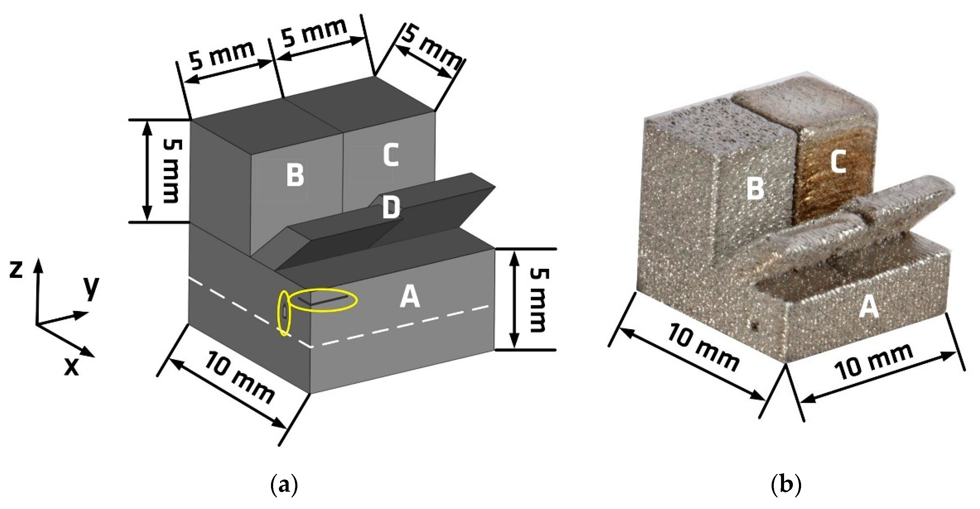
2.1.2. Description of the Specimen and Processing Parameters

Figure 2 illustrates the geometry of the specimen. It can be described by two cubes (B and C) of 5 mm edge length on top of a base cuboid (A) of the dimensions 10 mm × 10 mm × 5 mm, as cubes of this edge length are often used for L-PBF parameter studies. It also kept the field of view small for the optical monitoring equipment. Next to the cubes B and C inclined ramps (D) with an inclination angle of 40° and 45°, respectively, were placed. However, these ramps D were not subject of investigation in the course of this study. The specimen was removed from the build base plate by saw-cutting, the approximate position of the cutting line is depicted by the white dotted line. The base cuboid A contained artificial defects: In layers 61–73, an area of 0.6 mm × 3 mm was not exposed to the laser scan, followed by a non-exposed area of 0.37 mm × 3 mm in layer 74 at the same x-y-position. This region was called cavity in the course of this study. In layer 88, an area of 1 mm × 2.04 mm was not exposed at one corner. Both defects were open defects in the meaning that they were not enclosed within the part but are located at the edges.

A stripe scanning pattern with a maximum stripe length of 10 mm was used as scanning strategy for the entire part with scanning vectors parallel to the specimen’s edges. A rotation of the scanning vectors by 90° from layer to layer was applied. The hatch distance was set to 0.12 mm. No separate contour scanning was conducted, but a border offset of 0.08 mm was used, resulting in a separation of the single volume sections in x-y-direction on top of the base cuboid A. Three distinct scan parameters were used to produce the different volume sections to enforce the development of typical L-PBF defects during the process. While volume A was exposed by a parameter set which is normally used for high quality parts, volumes B and C were exposed by parameters resulting in a much lower or a much higher volumetric energy density (VED), as defined in [9]. The specific parameter sets are listed in

Table 1. L-PBF (laser powder bed fusion) parameters used for the different sections of the specimen.

Parameters of Sections	A	B	C
Parameter Set	Standard volumetric energy density (VED)	Low VED	High VED
VED in J/mm³	65.5	35.7	152.7
Laser Power PL in W	275	150	275
Scanning Velocity vs in mm/s	700	700	300

. From previous investigations, the applied parameter sets were known for creating lack-of-fusion defects (in case of low VED, volume B) or keyhole porosity (in case of high VED, volume C).

2.2. In-Situ Monitoring by Thermograpy and Optical Tomography

2.2.1. Optical Setup

For the in-situ monitoring of the L-PBF process, two different cameras were used simultaneously: A mid-wave infrared (MWIR) camera of the type ImageIR8300 (InfraTec GmbH Infrarotsensorik und Messtechnik, Dresden, Germany) sensitive in the spectral range from 2 µm to 5.7 µm was chosen for thermographic measurements. For optical tomography (bulb exposure of each layer exposition [30]), a CMOS camera of type M4020 (Teledyne Digital Imaging Inc., Billerica, MA, USA), which works in the visible and near infrared spectral range (VIS NIR), was used. It was equipped with a bandpass filter having a central wavelength of 880 nm and a spectral width of 50 nm. The cameras met the requirements of having a high enough spatial resolution to monitor on a melt track range of size (hatch distance was 120 µm) at different wavelengths. The second requirement of enough temporal dynamics to acquire information of cooling behavior is met by the MWIR camera at the displayed configuration. Figure 3 schematically depicts the optical setup. Both cameras were placed outside of the build camber on top of the machine and observe the same region of the build plate via a beam splitter through a sapphire window in the ceiling of the build chamber. Additionally, two gold mirrors were mounted at the ceiling inside the chamber using standard mounting plates which were screwed at the chamber ceiling. They offset the optical path to allow for a less inclined (close to parallel to the build plane) observation plane of the field of view (FOV). In addition, they enabled a comfortable selection of the FOV by manual adjustment of the mirrors. More technical data of the cameras are listed in

Table 2. Technical data of the used cameras.

Camera System	Thermography	Optical Tomography
Camera	Infratec ImageIR8300	DALSA Genie Nano-M4020
Detector	cooled InSb-focal-plane array	CMOS
Detector Size	640 × 512 pixels	4112 × 3012 pixels
Used Detector Elements	192 × 176 pixels	4112 × 3012 pixels
Lens Focal Length	100 mm	50 mm
Resulting Optical Resolution	100 µm/pixel	50 µm/pixel
Framerate and Exposure Time	900 Hz, 90 µs	bulb exposure of layer expositions
Effective Sensitive Spectral Range	2 µm–5.7 µm	855 nm–905 nm
Black Body Calibration Range	623 K–973 K	no calibration

. The maximum size of the FOV of the set-up in its presented configuration was limited by approx. 64 mm × 51.2 mm for the MWIR camera.

2.2.2. Data Acquisition

For MWIR thermography, a thermal video of each layer exposition was recorded using a framerate of 900 Hz and an optical resolution of approximately 100 µm per detector element on the build surface. The acquisition of each layer was started by using a software trigger, which launched the recording when the signal of a single pixel in the image was above a certain threshold value, with pretrigger function. For the OT, the VIS NIR camera was operated in bulb mode, i.e., it was integrating intensity during a high level at the trigger input. Thus, an uninterrupted high-level signal during each layer exposition was needed. To this end, an analog output of the L-PBF machine that is proportional to the laser output power was processed by low pass filtering to remove short low-level phases during the time of jump vectors in between hatch vectors. A subsequent use of a Schmitt-Trigger ensured a high level of well-defined voltage. This signal processing, especially the lowpass filtering, led to a short delay between the first laser activation of a layer exposition and the start of the camera acquisition. Thus, a small dummy part was built outside the FOV of the cameras, that was always exposed first in each layer to counteract this delay. As a result, the camera chip was exposed from shortly before the start of the exposition of the part in the FOV until shortly after exposition for each layer.

The thermographic videos of the build process presented a very large amount of data containing a lot of information, e.g., the size of this study’s thermographic data was 12 GB for a sample cube of 10 mm edge length, despite data compression. Extracting the most useful information for a certain monitoring objective is a very challenging task. In this study, only first qualitative and manually obtained results regarding the detection of defects are presented.

2.3. Ex-Situ Inspection by Computed Tomography, Metallography and Data Integration

The specimen was inspected by a custom-made industrial 3D micro CT scanner. This scanner was equipped with a 225 kV micro focus X-ray source (X-ray WorX GmbH, Garbsen, Germany) and a flat panel detector with 2048 × 2048 pixels. More details about this micro CT scanner can be found in [33]. The achieved voxel size of 7.12 µm enabled the detection of defects with a diameter larger than 14 µm. The commercial software VG Studio Max 3.1 (Volume Graphics GmbH, Heidelberg, Germany) was used to analyze the µCT data. The whole specimen was scanned. The volume of the volumes A, B and C was determined within VG Studio 3.1. The volumetric porosity in each 3D dataset of the three volumes was calculated using VG studio’s porosity analysis module.

In addition to non-destructive inspection by µCT, destructive metallography was used to analyze the specimen. Therefore, polished cross sections of the specimen were etched using Beraha II etching detergent for 10 s to 30 s. Measurements of melt pool depth were conducted at light-microscopy micrographs for the three distinct parameter sets used in volumes A, B, and C. Light-microscopy was conducted using a Polyvar Met (C. Reichert Optische Werke AG, Wien Austria) which was equipped with a camera DFC290 (Leica Microsystems GmbH, Wetzlar, Germany).

The image registration software elastix 4.9 (University Medical Center Utrecht, Utrecht and contributors, The Netherlands) by Klein et al. [34] was utilized to overlay the extracted datasets of thermography and optical tomography onto the µCT data. Even though it is most frequently used in medical applications, it was well suited for the purpose of this study. It utilized affine transformation with the results getting visualized in Amira ZIB Edition 2019 (Thermo Fisher Scientific, FEI SAS, Illkirch-Graffenstaden, France).

3. Results and Discussion

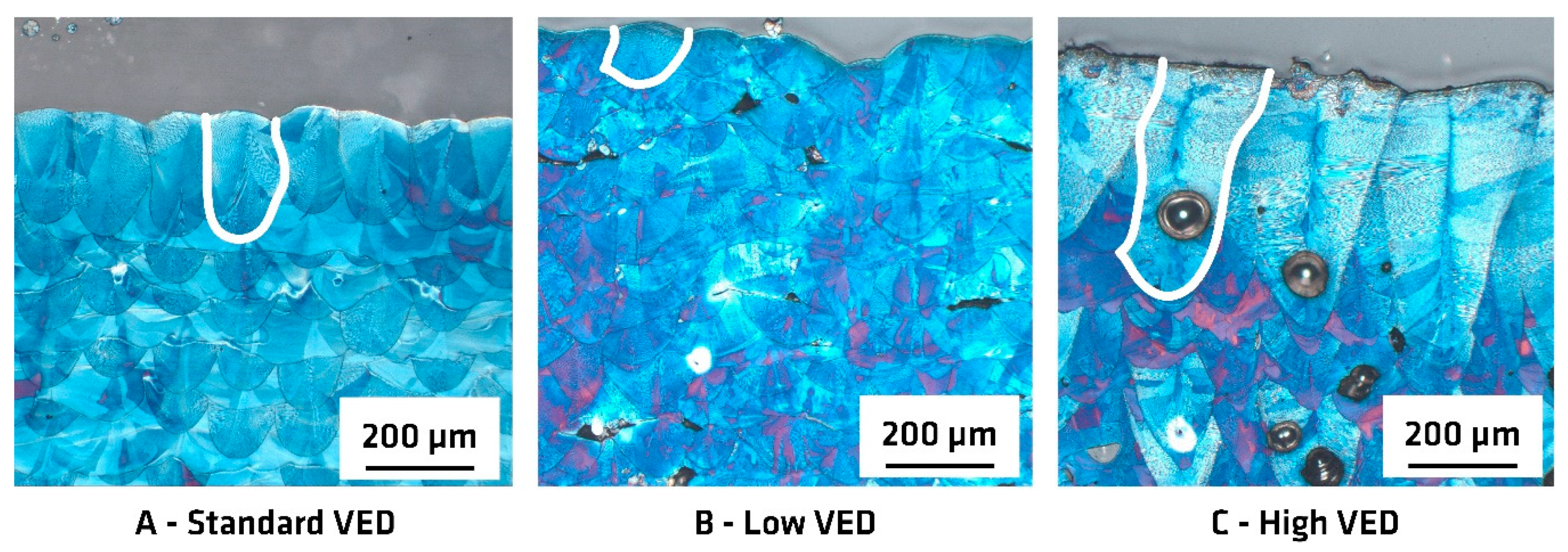
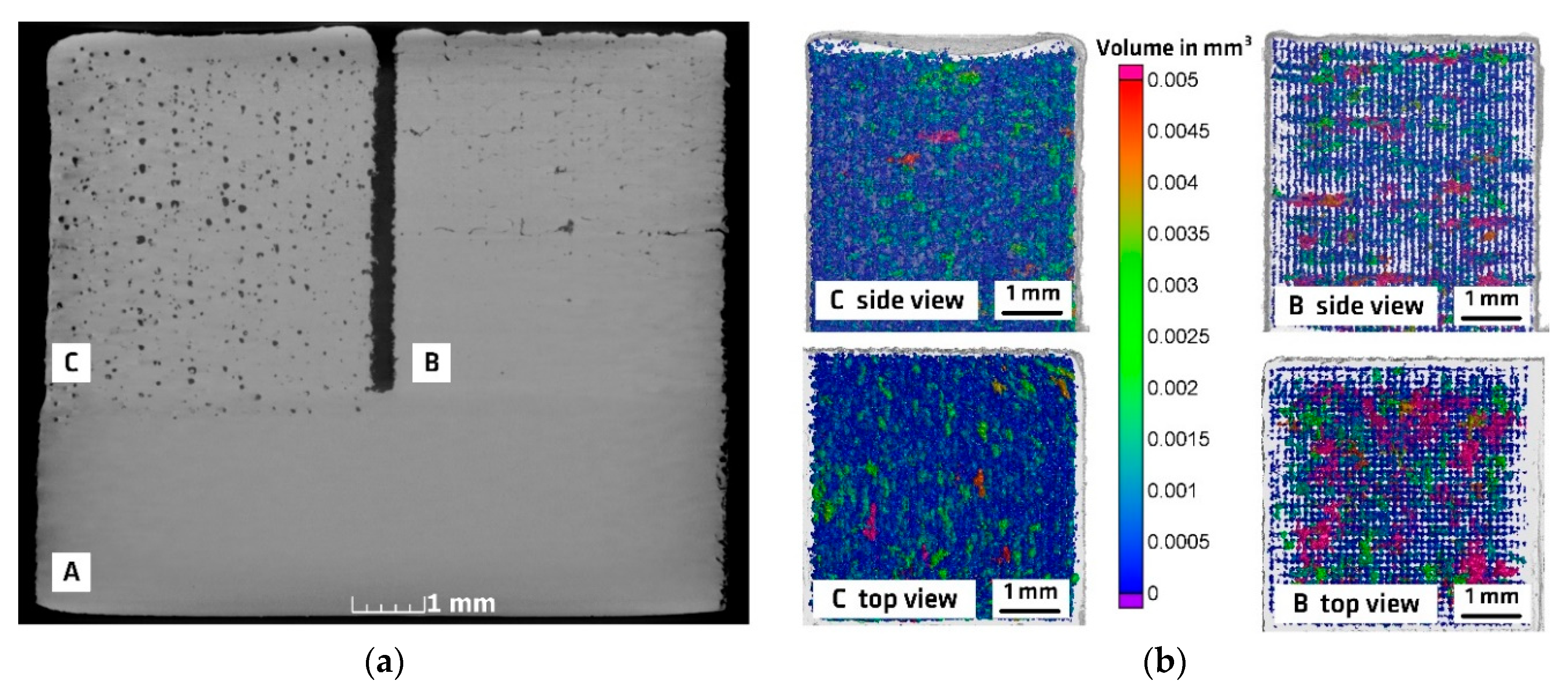
3.1. Influence of Processing Parameters Analysed by µCT and Metallography

The ex-situ inspection of the specimen confirmed the expected presence of distinctive internal defects due to the variation of the VED in the volumes A, B and C. In addition to defect development, the melt pool depth and shape was influenced by the differences in VED, which is exemplified by the white lines in Figure 4 right depicting the melt pool boundaries of the top layer. Grain size determination was not in the focus of this study. Quantitative measurements from metallography (mean of ten melt pool depths of the topmost layers) and µCT (porosities with diameter larger than 14 µm) are summarized in

Table 3. Quantitative measurements of melt pool depth and porosity percentage.

Melt Pool Depth and Porosity in Different Sections	A	B	C
Parameter Set	Standard VED	Low VED	High VED
Melt Pool Depth in µm	213 ± 19	117 ± 14	471 ± 54
Pore Volume in % of Part Volume Measured by µCT	<0.1	2.7 *	7.4

* Underestimation of the real value due to partly entrapped powder in the voids.

.

Qualitatively, the three parts could be described as: free of major defects (A), containing lack-of-fusion voids (B), containing keyhole porosity (C), as depicted in Figure 4 and Figure 5. Due to the huge penetration depth of the laser in volume C and the resulting melt pool depth, which is considerably deeper than the layer thickness (factor 9), some keyhole pores could also be found in cuboid A underneath the cube C. The pores and voids of the cubes B and C, lack-of-fusion voids and keyhole pores, respectively, showed typical morphological differences: Keyhole pores, as entrapped vapor pores, are characteristic for deep penetration welding when having unstable welding conditions. They are predominately of spherical shape. Lack-of-fusion voids develop due to insufficient fusing of the molten powder material between the adjacent melt tracks and layers. They have predominately irregular and sharp shapes. More information about these well-known defects in L-PBF can be found in the literature, e.g., [11,16,35].

The scanning strategy determined the distribution of the pores. Keyhole pores were found predominately in-line with the scanning vector, whereas the lack-of-fusion voids were mainly located between adjacent scanning lines. Due to the chosen scanning pattern with stripes rotated by 90° after every layer, a clear pore or void pattern was observed in µCT data. In addition to these repeated defect patterns, bigger defect clusters were also observed within the cube B. Both are visualized in Figure 5. Missing distinctive reference points due to solidification shrinkage of the part complicated a precise layer-wise comparison of the data sets from process monitoring and µCT.

3.2. In-Situ Monitoring

3.2.1. Data analysis Concepts

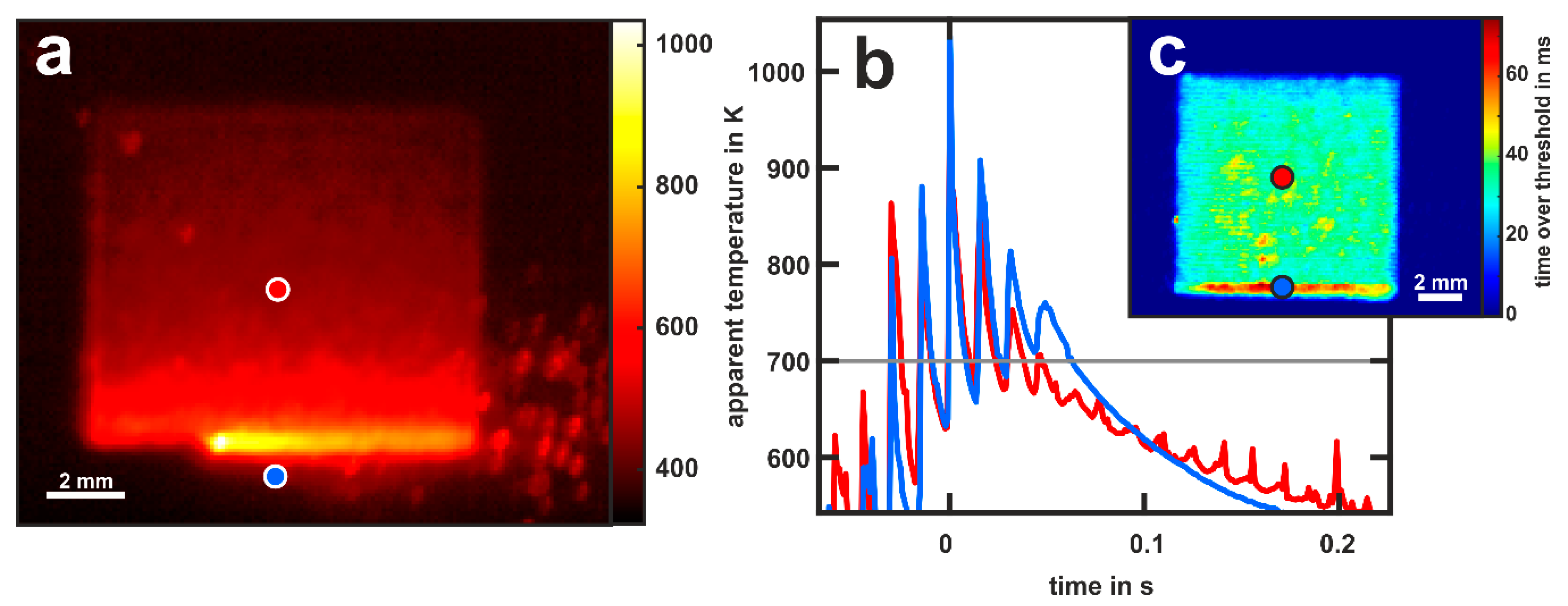
Thermography–Apparent Temperatures

Since the MWIR camera was calibrated for black body radiation by its manufacturer, the temperatures that were acquired in this work were only apparent temperatures and well below the actual temperatures in the process. There were a number of reasons for this: Firstly, the emissivity of the melt pool, the built part surface and the powder are well below unity, the case for which the camera calibration is valid. For example, the emissivity value depends on surface roughness, wavelength, oxidation state and state of matter. For the used material AISI 316L in the unoxidized solid state, values of the total hemispherical emissivity between roughly 0.25 and 0.35 were expected [36]. In addition, to the material dependent emissivity, differences in heat conduction and heat capacity as well as differences in the processability could lead to different results for other materials. Secondly, the optical elements in the optical path, i.e., the beam splitter, the gold mirrors and the sapphire window attenuated the emitted thermal radiation, which was not taken into account by the vendor calibration. Additional thermal radiation emitted from the optical elements themselves in the optical path may, however, be neglected in the current setup, since their temperature was close to room temperature and well below the lower calibration limit of the camera of 623 K. Thirdly, the limited spatial resolution of 100 µm/pixel of the setup led to an additional error in the temperature calibration. The extremely high spatial temperature gradients on the surface caused each detector element to measure an average intensity of the corresponding area of the build surface. Since the relationship between intensity and temperature is strongly non-linear, the acquired temperature close to and within the melt pool was not an average temperature of this area but it was rather overestimated. Contrarily, if one is interested in the maximum temperature in the melt pool, this value will be underestimated since the spot size of the maximum temperature was expected to be much smaller than 200 µm × 200 µm, which would be the needed minimum size to avoid spatial undersampling. However, these resolution-dependent effects diminished with cooling down after solidification, since the spatial thermal gradients diminished as well.

As the temperature values given by the camera calibration were not valid, the analysis of the raw data intensity values of the camera would have been an opportunity instead. However, in that case, the strong nonlinearity of the intensity-temperature dependence would have complicated the data analysis and other methods to reduce the signal dynamics would have been required, such as analyzing the logarithm of the signal. Instead, in the course of this study, the apparent temperatures as given by the camera were analyzed. Therefore, the measured temperature values and measured temperature differences were only apparent.

Figure 6 gives an overview of typical thermographic data. Figure 6a shows a single thermogram of the process, illustrating that there was a certain amount of spatter ejected from the melt pool traveling through the image, which might complicate certain image processing steps. Figure 6b shows the time development of the apparent temperature at two different single pixel positions in the sample, as depicted in Figure 6a,c. As expected for the chosen build parameters, the apparent temperature rose multiple times, thus each volume element was reheated several times during each layer exposition.

Thermography–Time over Threshold (TOT)

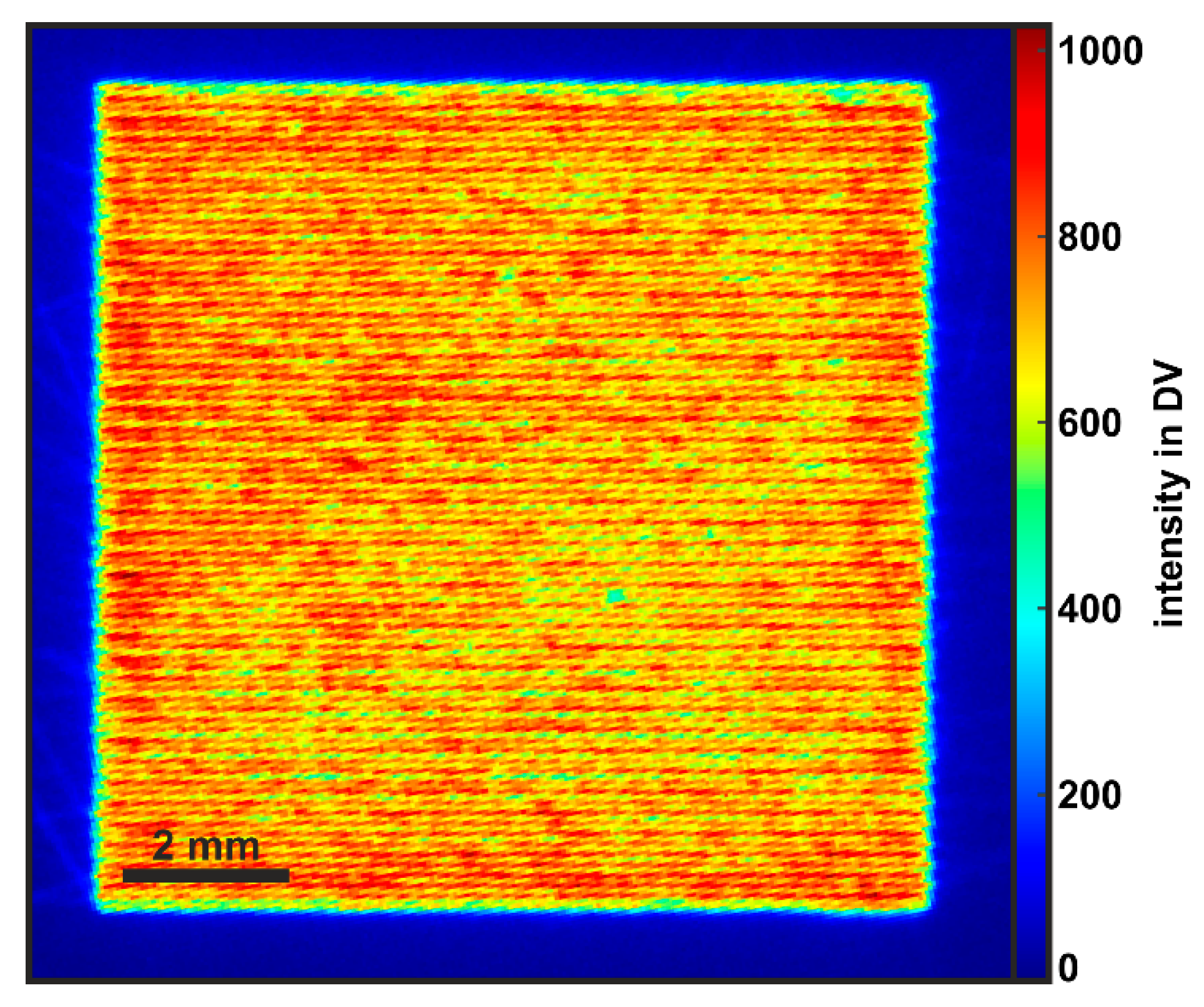
Here, as a feature extracted from the thermographic data, the focus was set on the time a surface element of the specimen had an apparent temperature above a certain threshold value during the build of the respective layer, called time over threshold (TOT). This value could easily be extracted from the data. TOT showed increased (reduced) values if the cooling rate was decreased (increased) in the relevant temperature regime, depending on the chosen threshold value. Such deviations would have been expected if significant process deviations from the ideal case leading to defect formation were present. However, different kinds of defects or their formation mechanisms as well as the part geometry itself might influence the TOT in different ways. For example, the ejection of loosely bounded material that cools down relatively slowly leads to a locally strongly increased TOT directly in the layer of occurrence. In the subsequent layer, however, a small increase in TOT at this location gets possibly registered, due to heat accumulation above the defect. In contrast, the incomplete melting of powder leads to lack-of-fusion pores which might only lead to an increase of TOT in the subsequent layer and not in the layer of origin. Thus, for a thorough understanding of the process and its influence on the TOT, thorough studies are needed. The first results are presented here.

In Figure 6c, a map of the TOT of an apparent temperature of 700 K is shown for the layer formation of Figure 6, which did not contain any defects, as found by reference measurements. The increased TOT at the lower side of the image was caused by a reduced cooling rate in this area, probably due to a heat accumulation due to the absence of solid material on the further lower hand side (only powder with reduced thermal conductivity is present here). Contrarily, as observable in Figure 6b, the final cooldown at the end of the exposition (blue curve) was faster, since the laser stopped the continuous heating of the part after the last scan track was exposed.

In fact, Lough et al. [37] also performed this kind of time over threshold analysis in the L-PBF process. However, they did not show a correlation between actual defects in the samples and this quantity. They chose the intensity of the solidification temperature plateau as a threshold value and analyzed the intensity values directly. In the present study, the framerate of the thermographic video was insufficient for the use of such a high temperature as threshold value. The maximum apparent temperature of the melt pool moved several pixels between subsequent frames and a strong stroboscope effect became visible in the TOT map due to temporal undersampling. Thus, a threshold value of 700 K was chosen for the analysis, since it was close to the highest possible value without being affected by stroboscopic effects. The presented correlation between extracted features and real defects in the final part was rather phenomenological and the spatial overlap between lack-of-fusion pores and TOT values was best for higher values, which were not affected by stroboscopic effects.

Optical Tomography

Contrary to thermography, the optical tomography camera recorded only a single image per layer exposition. Optical tomography recorded a signal which was proportional to the radiation intensity, emitted from the area on the specimen that was imaged onto the respective detector element (pixel), integrated over the duration of the entire layer exposition. Under normal process conditions, the highest temperatures within the melt pool would have contributed predominantly to the signal due to the nonlinearity of the temperature-intensity dependence despite the very rapid cooling. Therefore, the hatching pattern of the layer exposition can be seen in the optical tomography images, as depicted in Figure 7. However, since the measured signal was only proportional to the time integral of the intensity, it could not be distinguished between areas on the build surface that had an unusually high temperature and those that had an unusually low cooling rate at moderate temperatures. Nevertheless, both occurrences might have been indications for process deviations that might have induced the formation of defects. Thus, for defect detection, threshold analysis operating on the raw signal data were applied.

3.2.2. Influence of Processing Parameters on In-Situ Monitoring Signatures

Standard Process Parameters

In the base volume A built with standard parameters, only small spatial deviations were observed in the TOT maps and OT images. Figure 8 shows TOT maps of two different layers in volume A, i.e., the first exposed layer (layer 1, Figure 8a) and the last horizontally exposed layer (layer 99, Figure 8b). Three regions of interest (ROIs) are marked for further analysis: A region at the upper hand side of the part, which was exposed at first (red), the center region (gray) and a region at the lower hand side, which was exposed at last (blue). The mean TOT values developed in these regions with increasing layer numbers as depicted in Figure 6c. Two main observations could be made: Firstly, the average value of the TOT was lowest in layer 1, which could be explained by the decreasing cooling rate for increasing built height. In layer 1, the heat could be conducted directly into the substrate plate, while in layer 99 it had to be conducted through a reduced cross section, i.e., the geometry of the already built part, which was thermally insulated laterally by the surrounding unmolten powder. In addition, with repeated heating of the growing part by melting of further layers, the temperature of the part rose initially. This effect could be seen for all three ROIs in Figure 8c. Secondly, in layer 99, the TOT in the lower ROI (blue) was considerably increased compared to the other ROIs, which was not observable in layer 1. As explained in Section 3.2.1 this feature was caused by the lowered heat conduction into the built part, due to the lack of solid material at the further lower hand side. This hypothesis was supported by the absence of this TOT increase in the first layers and the increasing difference between the TOT values of the upper ROI (red) and the middle ROI (grey) in subfigure c. Here it could also be seen that the TOT in the upper region was always lower than in the other ROIs, which was consistent with higher expected cooling rates at the beginning of a layer exposition due to missing heat accumulation during the layer exposition in the built part and substrate plate.

It should be noted that all the observations mentioned so far were explainable and not surprising, however, they were also inherent to any build and did not cause any defect formation in the magnitude of intensity as observed here. Nevertheless, overheating due to geometry effects might lead to defect formation in more extreme cases of complex structures.

The OT image of layer 99 (same layer as shown in Figure 8b) is shown in Figure 7. There were no indications of differences observable in the signal between the different ROIs defined in Figure 6. This was consistent with the observation that the increase in the TOT for a threshold value of 700 K at the lower region of the part (blue ROI) were caused by a moderately decreased cooling rate at intermediate apparent temperatures close to 700 K (compare Figure 6b), while the OT signal was dominated by the intensity of the highest temperatures of the melt pool.

Comparison between Standard, High and Low VED Settings

In the volumes B and C, the mean values of the OT intensity and the TOT (700 K) deviated considerably from the values of the volume A. The mean values are given in

Table 4. Mean values of the in-situ measurement results for the volumes with different energy density settings. The mean values were calculated for areas well within the respective volumes in order to avoid the influence of edge effects.

Volume	A	B	C
Parameter Set	Standard VED	Low VED	High VED
Mean TOT(700 K) in ms	28.1	14.5	280
Mean OT Signal in Digital Values (DV)	816	483	2860 *

* Underestimation of the real value due to partially oversaturated signal.

.

The detector intensity was occasionally saturated in the high VED volume C so its values of OT intensity were rather a lower limit. Since the defects that were created in volume C were quite uniformly distributed and no significant clustering occurred that might have been observable in the in-situ monitoring for correlation (see Section 3.1), the data from volume C was not further analyzed. Additional studies to investigate the onset energy density for keyhole pores and the corresponding in-situ monitoring signatures are currently being performed.

In the low VED density volume B, there were certain spatial signatures in the in-situ monitoring data that correlated with particularly large defects, as observable in the µCT data. They are discussed in the following section.

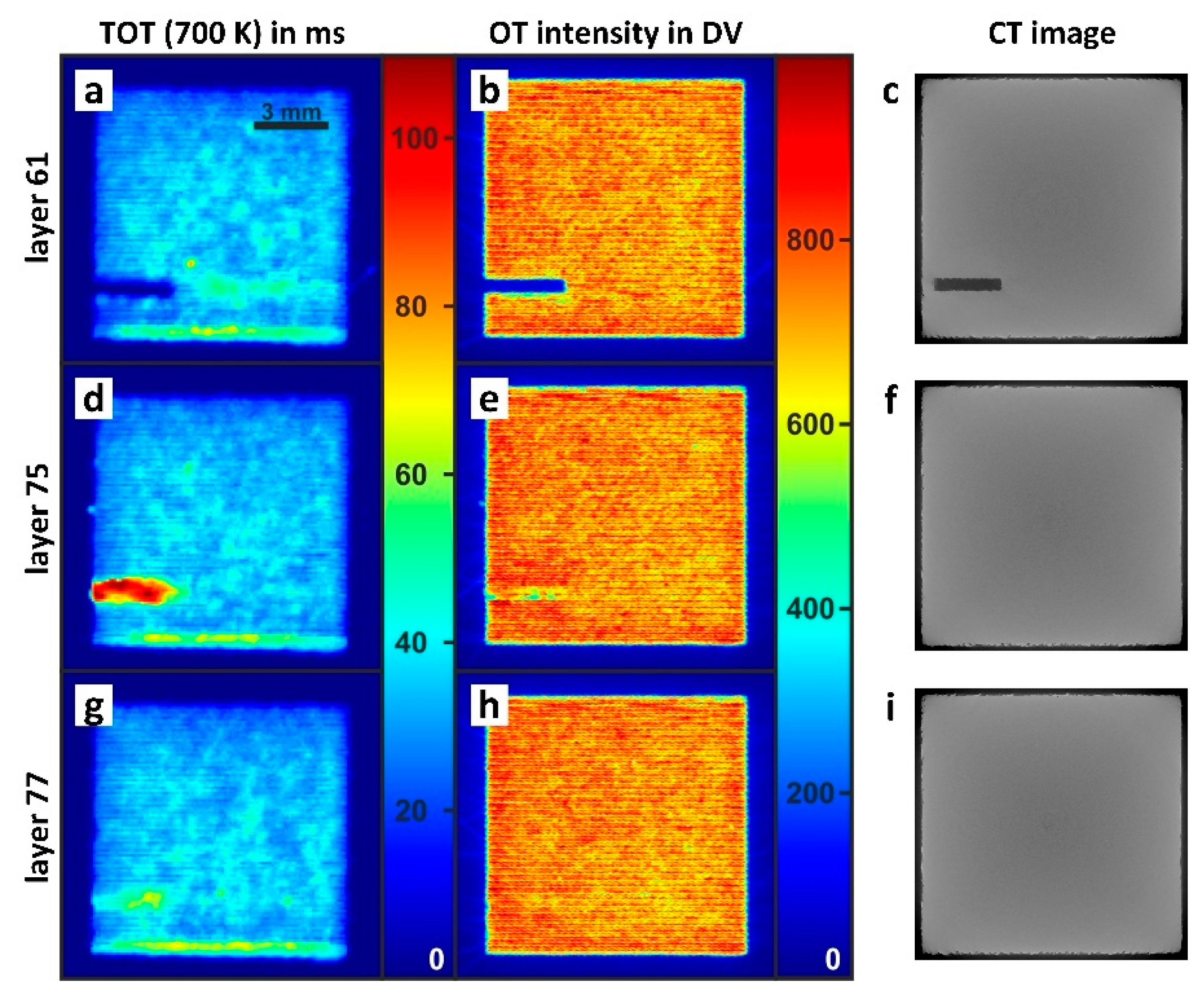
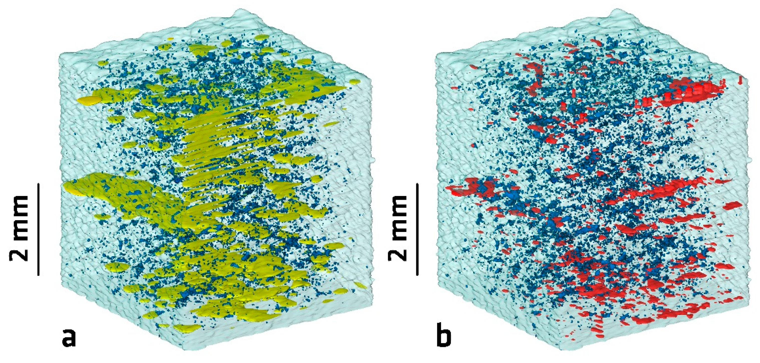
3.2.3. In-Situ Monitoring for Defect Detection

Processing Parameters Related Defects

In volume A (standard processing parameters), µCT data showed no defects, except for single, individual pores and the region directly below Volume C (see Figure 5). Thus, a comparison to the in-situ monitoring data showed that any signatures as they occurred during the manufacturing of this volume were indicative of a stable process. In particular, TOT (700 K) values of up to 60 ms, as occurring at the lower rim of volume A (see Figure 6c), were not a sufficient single indicator for the formation of part density related defects.

As described in Section 3.1, in volumes B and C, the development of pores and voids was directly provoked by the purposely chosen processing parameters and the applied scanning strategy, which led to partially unstable process conditions. As explained above, the porosity distribution in volume C (high VED) did not show any clearly localized signatures in µCT that would allow for a comparison of the in-situ results spatially resolved to the µCT data. Strongly increased values of OT intensity and TOT (700 K) were found, but further studies are needed for reliable local defect detection.

Contrary, in volume B, despite the low average VED, there were larger volumes without or with only minor porosity, as shown by µCT. However, there was also a number of small lack-of-fusion defects and large clusters of lack-of-fusion defects. Thus, a comparison of specific signatures in the in-situ data with the defect structure in the µCT data was promising. So far, this was conducted qualitatively and manually and is exemplified for two layers, which showed some nesting of porosity in particular areas, see Figure 9. In addition to the OT intensities and the TOT (700 K), intensity maps extracted from the commercial MPM system are also depicted. All three measurement systems showed an increase of the respective signature with respect to the average signature value of the layer at similar x-y-positions. A qualitative comparison to the respective µCT cross sections revealed increased occurrence of porosity at these positions. As a guide to the eye, a contour plot for a threshold value of 30 ms in the TOT (700 K) map is overlaid in the maps of the other signatures and shows a high correlation to the defective region in the µCT map. Interestingly, the value of 30 ms was significantly higher than the mean TOT (700 K) value of 14.5 ms in volume B, but close to the mean value of the TOT (700 K) value in the defect free volume A, which was manufactured using standard parameters. Thus, for a definitive defect detection, the TOT (700 K) alone was no clear indication for defect formation and at least a second criterion would be needed, possibly also extracted from the thermographic data or from another technique, e.g., indicating the operation in lack-of-fusion mode. Similarly, for OT, the intensities at the locations of the defects were well above the mean value for volume B (483 DV), but well in the range of volume A (mean value of 816 DV). Additionally, the correlation with the defect geometry from µCT appeared to be worse compared to the TOT (700 K). For the MPM system, the correlation to the defects from µCT appeared to be even better than the TOT (700 K), but the lack of knowledge about the nature of the displayed signal and the impossibility to export the data for further analysis hindered a more thorough analysis. Lack of fusion voids as unfused material underneath the layer of exposition seemed to reduce the heat conduction which results in heat accumulation in the current layer that can be measured as thermal signal deviation. This effect is discussed in the following paragraphs in more detail.

Artificial Defects with Standard Process Parameters

In addition to deviations of process parameters as source of defect development, defects can also arise from overheating caused by geometrical effects. The cavity in layers 61–74 (described in Section 2.1), which was not exposed, was clearly visible in the acquired data, as depicted in Figure 10. An increase of the TOT (700 K) was registered on top of this cavity in the first subsequent layer, which was exposed completely again, i.e., layer 75. This showed the heat accumulation at this position, caused by reduced heat conduction due to unfused material underneath. A slight increase of the TOT signal was still observable in layer 77. Thus, additional information, which is in this case information about part’s geometry, is needed to guide the analysis of the TOT data.

The strong signals caused by the artificial cavity illustrated the reduction of heat conduction caused by large defects which might have had an influence on a number of subsequent layers. The µCT images of the respective layers 75 and 77 did not show any defects. However, the exact determination of the layers in µCT was hindered due to shrinkage and missing reference points. Thus, a clear determination of the actual z-position of a detected defect in the part might have an uncertainty of one or two layers at the current state of research. The mentioned uncertainty of layer determination in the µCT dataset hindered a more detailed analysis of the defect position for this specimen. Follow-up experiments, allowing more accuracy in position correlation are planned. A detection of defects only during the exposure of layers above the defect containing layer would impede the possibility of real time control or repair as a desired action once monitoring works reliably, since a direct remelting of the damaged layer might not be possible at this late time of detection without adjustment of the scanning parameters. However, owing to the penetration depth of the laser as well as time for recoating, which can be used as calculation time, the potential of remelting for in-process rehabilitation of detected defects should not be neglected.

Furthermore, a corner in layer 88 of volume A was not exposed. Whereas the missing laser-material interaction was detected by the monitoring equipment in layer 88, no signal deviations was found at this region in the subsequent layer. This perfectly matched the µCT data and metallographic examinations of this region, which did not detect any defects related to the missing exposition in or in close proximity of this region in layer 88. In this case, a kind of self-healing occurred. During the build process, the laser remelted several subjacent solidified layers. Therefore, the unmolten powder particles in that corner were melted by the laser exposition of the subsequent layer. Surprisingly, no signal deviations were registered at this corner in layer 89, where the layer thickness had been twice the standard value of 50 µm resulting in a reduction of the local VED by half. This example showed potential sources of misinterpretation: On the one hand the exposition defect was healed by the laser exposition of subsequent layers but appeared in the layer of its origin. On the other hand, the sensitivity for low energy inputs has to be improved for the applied data examination strategy, as no deviations in layer 89 were detected by using the described threshold values. Both examples of artificial defects clearly indicated the necessity of knowledge about the geometry and slice pattern of a part during the analysis of monitoring data.

3.3. Automation of Data Handling

Image registration was used to reduce the spatial uncertainty and to allow data comparison, which is important to identify signal thresholds for defect detection. The upcoming section presents first results of this process with a focus on volume B. Further work in the field of data integration will be conducted and reported in a subsequent study.

Image registration was utilized to overlay data from different imaging modalities which differed in recording conditions and spatial resolutions, especially in the build direction. It was also important to indicate, that the camera-based data were captured during the manufacturing process in contrast to the µCT data, which were acquired after the process. Therefore, the in-situ data were not able to account for possible shrinkages, warpages and other deformations. Hence, registration was needed.

The choice of transformation represented an important aspect of the registration process. The type of transformation determines how a dataset, e.g., a specific TOT, is deformed to match the shape of another dataset, in this case, µCT data. Two transformations were considered for this paper: rigid (Euler) transformation and affine transformation. Rigid transformation allows rotation and translation of a dataset, only. Therefore, it was not able to describe uncertainties in the exact pixel size of thermography and optical tomography data, which might have led to mistakes in the transformation, and spatial deviations due to solidification shrinkage. Affine transformation added the possibility of scaling and shearing. Thus, it could be applied to compensate uncertainties in pixel size but failed to describe irregular solidification shrinkage or other geometrical discrepancies.

Thermography and OT data were registered onto the µCT data to compare the two methods. The advanced Mattes mutual information metric [38] was used, utilizing a Gaussian pyramid scheme. Figure 11 shows the results of 18,500 iteration steps. Affine transformation was able to match the edges of the specimen more precise than rigid transformation since it could adjust to measurement uncertainties of the optical system’s pixel size. Therefore, it was used for visualization.

A virtual envelope of the specimen was utilized to guide a user during the analysis of the datasets. The µCT scan was selected to shape the envelope because it represented the geometry of the produced specimen. The watershed segmentation method in the Amira software was applied to determine the specimen’s surface based on the edge image of the µCT dataset. Amira’s Auto Threshold module was used to visualize the pores in µCT data: The implemented method of Otsu et. al. [39] automatically computed a threshold for binary segmentation based on the histogram of the 256 grey values of the 8-bit µCT data. Otsu’s method is a simple but effective method to compute a single threshold separating a set of values into two classes. The threshold computed by Otsu’s method minimizes the intraclass variance and, hence, maximizes the interclass variance. Taking the defects as defects of the same kind building a continuum rather than separate classes, two classes in the data needed separation. Under the assumption that only two classes were present in the data, the computed threshold was the best achievable value for a single threshold. Segmented lack-of-fusion pores were visualized as a binary image containing all voxels below the calculated threshold of 80. In contrast, defects in the optical tomography and thermography data were extracted by manually choosing a suitable threshold for Volume B.

Lastly, Amira’s surface rendering module was used to display a transparent version of the specimen’s surface, pores segmented from µCT data and occurring optical tomography signal of over 700 DV and TOT (700 K) greater than 30 ms. This is illustrated in Figure 12. A first analysis of the images in Figure 12 revealed that there was only a small volumetric overlap between porosity and the anomalies detected in thermography and OT. This was not surprising since the thermal signals as pseudo-3D-volume elements were not to be expected to overlay directly to 3D volumes of pores as real volumetric defects and even less to overlay completely. Defects below the actual monitored layer affected the thermal signals due to influence on thermal conduction. However, due to the complex morphologies of the defects, this influence was not expected to be homogeneous over the entire cross-section of a defect. Nonetheless, a quick analysis of the overlap of thermal signal anomalies and pores was conducted as a basis for further in-depth analysis.

Table 5. Binary volumetric overlap of segmented pores from µCT data and anomalies detected by thermography (TOT (700K) > 30 ms) and OT (OT signal > 700 DV), where the relative cumulative volumes compared with respect to cumulative pore volume are 90% for thermography and 8% for OT.

Overlap of Signals and Defects	All Pores, 0 Layers Shifted	All Pores, 1 Layer Shifted	Pores > 0.001 mm³, 0 Layers Shifted	Pores > 0.001 mm³, 1 Layer Shifted
Micro-CT pores overlapped by thermography anomalies	3.1%	3.1%	35.1%	29.9%
Micro-CT pores overlapped by OT anomalies	0.7%	0.5%	14.3%	11.7%
Thermography anomalies overlapped by micro-CT pores	71.4%	55.5%	33.3%	30.2%
OT anomalies overlapped by micro-CT pores	17.1%	15.1%	11.0%	8.8%

presents the binary volumetric overlap, which classifies pores and anomalies as either found or not found by partial overlapping of each other, using two distinct ways of analysis: at first, the overlap of detected pores by thermal signal anomalies, as a measure of the likelihood of lack of fusion voids to be detected; secondly, the overlap of thermal signal anomalies by the detected pores, as a measure of the likelihood of signal anomalies to detect lack of fusion voids and not fully consolidated material. Besides, the same binary volumetric overlaps were analyzed for all pores larger than 0.001 mm³ and after shifting the datasets of thermal signals and µCT by one layer to account for the layer discrepancy between the occurrence of a defect and its detection. This analysis was conducted for the lower left quadrant of Volume B to avoid the influence of Volume C on the thermography data. Note that the cumulative volume of the anomalies detected with TOT (700 K) over 30 ms and OT over 700 DV comprised only 90% and 8% of the cumulative pore volume, respectively.

A rather low percentage of binary volumetric overlap could be observed between the volume of the lack of fusion voids segmented in the µCT data and the detected anomalies in TOT and OT. The percentage increased when neglecting small pores. The low percentage of binary volumetric overlap was particularly striking for OT and could be partially explained by the much smaller volume of the OT anomalies compared to pores segmented from µCT data. Furthermore, it seemed like the anomalies in OT occurred in the surrounding of the pores, rather than on top of them. The low numbers of binary volumetric overlap contained in Table 5 were only presented to inform about the informative value of rough estimations for defect detections of thermal monitoring equipment based on single signals only. A sophisticated threshold determination and sophisticated data fusion of different signals was not conducted yet (e.g., OT and TOT at different threshold values and different shifts in the z-direction). In addition, the surrounding of the thermal signals or measured defects was not enlarged by different radii during the overlapping analysis, which could have improved the detection rate at the expense of potential falsifications due to potential double counting of defects. However, the binary overlap of thermography signal anomalies by the detected pores of up to 71% appeared already very promising for further in-depth correlation approaches. When deeper analysis will be applied a detailed analysis of the uncertainty of the measurements will also be conducted. Questions regarding the position of the inspected specimen on the build plate, robustness of the measurements against spatter and possible falsifications due to process plume between the camera and the object will be analyzed. A more detailed look at specimens with larger built heights will also be applied, as this can lead to heat accumulation effects, which directly influences the thermal signals. The existing data will be used for further analysis of those topics in another study.

4. Conclusions

A new setup for in-situ off-axis monitoring by synchronous observation of a L-PBF process via optical tomography and infrared thermography using the same optical path through the ceiling of the build chamber was successfully tested. The built up of a specimen containing artificial defects as well as purposely chosen process parameter variations was monitored. The feasibility of the set-up to detect defects has been verified by a comparison with data obtained by micro computed tomography. Despite non-calibrated thermography temperatures, the concept of time over threshold (TOT), i.e., time over a defined apparent temperature, was able to detect process deviations, which could be correlated to lack-of-fusion void clusters in qualitatively good agreement to µCT data for particular layers. In addition, a comparison to commercial monitoring equipment described the high potential of the presented setup as an independent monitoring solution with total data access. Due to the synchronous use of the distinct cameras, the advantages of a high spatial resolution (OT, here 50 µm/pixel), and relatively high temporal dynamics (thermography, here 900 Hz) were combined.

The manually and phenomenological data analysis approach constituted a basis for automated in-depth evaluation by data fusion. Although a first attempt of automated data integration showed a promising binary overlap of thermography signal anomalies and detected pores of up to 71%, the conducted data integration attempt revealed the need for data fusion concepts as single signal values seemed to have only comparably low spatial overlapping between signal and detected defects for the entire of a sub-volume of the monitored specimen.

References

1. Kruth, J.P.; Levy, G.; Klocke, F.; Childs, T.H.C. Consolidation phenomena in laser and powder-bed based layered manufacturing. CIRP Ann. 2007, 56, 730–759. [Google Scholar] [CrossRef]
2. Schmidt, M.; Merklein, M.; Bourell, D.; Dimitrov, D.; Hausotte, T.; Wegener, K.; Overmeyer, L.; Vollertsen, F.; Levy, G.N. Laser based additive manufacturing in industry and academia. CIRP Ann. 2017, 66, 561–583. [Google Scholar] [CrossRef]
3. Bourell, D.; Kruth, J.P.; Leu, M.; Levy, G.; Rosen, D.; Beese, A.M.; Clare, A. Materials for additive manufacturing. CIRP Ann. 2017, 66, 659–681. [Google Scholar] [CrossRef]
4. Herzog, D.; Seyda, V.; Wycisk, E.; Emmelmann, C. Additive manufacturing of metals. Acta Mater. 2016, 117, 371–392. [Google Scholar] [CrossRef]
5. DebRoy, T.; Wei, H.L.; Zuback, J.S.; Mukherjee, T.; Elmer, J.W.; Milewski, J.O.; Beese, A.M.; Wilson-Heid, A.; De, A.; Zhang, W. Additive manufacturing of metallic components—Process, structure and properties. Prog. Mater. Sci. 2018, 92, 112–224. [Google Scholar] [CrossRef]
6. Wohlers, T.T.; Campbell, I.; Diegel, O.; Kowen, J.; Caffrey, T. Wohlers Report. 3D Printing and Additive Manufacturing State of the Industry; Wohlers Associates, Inc.: Fort Collins, CO, USA, April 2007. [Google Scholar]
7. Spierings, A.B.; Dawson, K.; Voegtlin, M.; Palm, F.; Uggowitzer, P.J. Microstructure and mechanical properties of as-processed scandium-modified aluminium using selective laser melting. CIRP Ann. 2016, 65, 213–216. [Google Scholar] [CrossRef]
8. Karg, M.; Ahuja, B.; Kuryntsev, S.; Gorunov, A.; Schmidt, M. Processability of high strength Aluminium-Copper alloys AW-2022 and 2024 by Laser Beam Melting in Powder Bed. In Proceedings of the 25th Annual International Solid Freeform Symposium, Austin, TX, USA, 4–6 October 2014. [Google Scholar]
9. Mohr, G.; Johannsen, J.; Knoop, D.; Gärtner, E.; Hummert, K.; Emmelmann, C. Processing of a high-strength Al-Fe-Ni alloy using laser beam melting and its potential for in-situ graded mechanical properties. In Proceedings of the Lasers in Manufacturing Conference, Munich, Germany, 26–29 June 2017. [Google Scholar]
10. Tapia, G.; Elwany, A. A review on process monitoring and control in metal-based additive manufacturing. J. Manuf. Sci. Eng. 2014, 136, 060801. [Google Scholar] [CrossRef]
11. Grasso, M.; Colosimo, B.M. Process defects and in situ monitoring methods in metal powder bed fusion: A review. Meas. Sci. Technol. 2017, 28, 1–25. [Google Scholar] [CrossRef] [Green Version]
12. Rehme, O.; Emmelmann, C. Reproducibility for properties of selective laser melting products. In Proceedings of the Third International WLT-Conference on Lasers in Manufacturing, Munich, Germany, 13–16 June 2005. [Google Scholar]
13. O’Regan, P.; Prickett, P.; Setchi, R.; Hankins, G.; Jones, N. Metal Based Additive Layer Manufacturing: Variations, Correlations and Process Control. Procedia Comput. Sci. 2016, 96, 216–224. [Google Scholar] [CrossRef] [Green Version]
14. Zerbst, U.; Hilgenberg, K. Damage development and damage tolerance of structure maanufactuired by selective laser melting—A review. Procedia Struct. Integr. 2017, 7, 141–148. [Google Scholar] [CrossRef]
15. Rashid, R.; Masood, S.H.; Ruan, D.; Palanisamy, S.; Rahman Rashid, R.A.; Brandt, M. Effect of scan strategy on density and metallurgical properties of 17-4PH parts printed by Selective Laser Melting (SLM). J. Mater. Process. Technol. 2017, 249, 502–511. [Google Scholar] [CrossRef]
16. Sharratt, B. Non-Destructive Techniques and Technologies for Qualification of Additive Manufactured Parts and Processes: A Literature Review; Contract Report No. DRDC-RDDC-2015-C035 [Online]; Sharratt Research and Consulting Inc.: Victoria, BC, Canada, 2015. [Google Scholar]
17. Spears, T.G.; Gold, S.A. In-process sensing in selective laser melting (SLM) additive manufacturing. Integrating Mater. Manuf. Innov. 2016, 5, 16–40. [Google Scholar]
18. Alberts, D.; Schwarze, D.; Witt, G. High speed melt pool & laser power monitoring for selective laser melting (SLM®). In 9th International Conference on Photonic Technologies LANE; Bayrisches Laserzentrum GmbH: Fürth, Germany, 2016; Volume 2016. [Google Scholar]
19. Neef, A.; Seyda, V.; Herzog, D.; Emmelmann, C.; Schönleber, M.; Kogel-Hollacher, M. Low coherence interferometry in selective laser melting. Phys. Procedia 2014, 56, 82–89. [Google Scholar] [CrossRef] [Green Version]
20. Ali, U.; Mahmoodkhani, Y.; Imani Shahabad, S.; Esmaeilizadeh, R.; Liravi, F.; Sheydaeian, E.; Huang, K.Y.; Marzbanrad, E.; Vlasea, M.; Toyserkani, E. On the measurement of relative powder-bed compaction density in powder-bed additive manufacturing processes. Mater. Des. 2018, 155, 495–501. [Google Scholar] [CrossRef]
21. Grasso, M.; Demir, A.G.; Previtali, B.; Colosimo, B.M. In situ monitoring of selective laser melting of zinc powder via infrared imaging of the process plume. Robot. Comput.-Integr. Manuf. 2018, 49, 229–239. [Google Scholar] [CrossRef]
22. Anwar, A.B.; Pham, Q.-C. Study of the spatter distribution on the powder bed during selective laser melting. Addit. Manuf. 2018, 22, 86–97. [Google Scholar] [CrossRef]
23. Mohr, G.; Seeger, S.; Hilgenberg, K. Measurement of particle emissions in Laser Powder Bed Fusion (L-PBF) processes and its potential for in-situ process monitoring. In Proceedings of the Euro PM 2019, Maastricht, The Netherlands, 13–16 October 2019. [Google Scholar]
24. Dunbar, A.J. Analysis of the Laser Powder Bed Fusion Additive Manufacturing Process through Experimental Measurement and Finite Element Modeling; Open Access: State College, PA, USA, 2016. [Google Scholar]
25. Craeghs, T.; Clijsters, S.; Kruth, J.P.; Bechmann, F.; Ebert, M.C. Detection of Process Failures in Layerwise Laser Melting with Optical Process Monitoring. Phys. Procedia 2012, 39, 753–759. [Google Scholar] [CrossRef] [Green Version]
26. Zenzinger, G.; Bamberg, J.; Ladewig, A.; Hess, T.; Henkel, B.; Satzger, W. Process monitoring of additive manufacturing by using optical tomography. In Proceedings of the AIP Conference Proceedings, Boise, ID, USA, 20–25 July 2014; Volume 1650, pp. 164–170. [Google Scholar]
27. Bartlett, J.L.; Heim, F.M.; Murty, Y.V.; Li, X. In situ defect detection in selective laser melting via full-field infrared thermography. Addit. Manuf. 2018, 24, 595–605. [Google Scholar] [CrossRef]
28. Coeck, S.; Bisht, M.; Plas, J.; Verbist, F. Prediction of lack of fusion porosity in selective laser melting based on melt pool monitoring data. Addit. Manuf. 2019, 25, 347–356. [Google Scholar] [CrossRef]
29. Krauss, H. Qualitätssicherung beim Laserstrahlschmelzen durch schichtweise thermografische In-Process-Überwachung; Herbert Utz Verlag: Munich, Germany, 2017; Volume 325. [Google Scholar]
30. Bamberg, J.; Zenzinger, G.; Ladewig, A. In-process control of selective laser melting by quantitative optical tomography. In Proceedings of the 19th World Conference on Non-Destructive Testing, Munich, Germany, 13–17 June 2016. [Google Scholar]
31. Gögelein, A.; Ladewig, A.; Zenzinger, G.; Bamberg, J. Process Monitoring of Additive Manufacturing by Using Optical Tomography. In Proceedings of the 14th Quantitaitve InfraRed Thermography Conference, Berlin, Germany, 25–29 June 2018. [Google Scholar]
32. Mitchell, J.A.; Ivanoff, T.A.; Dagel, D.; Madison, J.D.; Jared, B. Linking pyrometry to porosity in additively manufactured metals. Addit. Manuf. 2020, 31, 100946. [Google Scholar] [CrossRef]
33. Oesch, T.; Weise, F.; Meinel, D.; Gollwitzer, C. Quantitative In-situ Analysis of Water Transport in Concrete Completed Using X-ray Computed Tomography. Transp. Porous Media 2019, 127, 371–389. [Google Scholar] [CrossRef]
34. Klein, S.; Staring, M.; Murphy, K.; Viergever, M.A.; Pluim, J.P. Elastix: a toolbox for intensity-based medical image registration. IEEE Trans. Med. Imaging 2009, 29, 196–205. [Google Scholar] [CrossRef] [PubMed]
35. Zhang, B.; Li, Y.; Bai, Q. Defect formation mechanisms in selective laser melting: A review. Chin. J. Mech. Eng. 2017, 30, 515–527. [Google Scholar] [CrossRef] [Green Version]
36. Hunnewell, T.S.; Walton, K.L.; Sharma, S.; Ghosh, T.K.; Tompson, R.V.; Viswanath, D.S.; Loyalka, S.K. Total Hemispherical Emissivity of SS 316L with Simulated Very High Temperature Reactor Surface Conditions. Nucl. Technol. 2017, 198, 293–305. [Google Scholar] [CrossRef]
37. Lough, C.S.; Wang, X.; Smith, C.C.; Adeniji, O.; Landers, R.G.; Bristow, D.A.; Kinzel, E.C. Use of SWIR Imaging to Monitor Layer-to-Layer Part Quality during SLM of 304L Stainless Steel. In Proceedings of the 29th Annual International Solid Freeform Fabrication Symposium, Austin, TX, USA, 13–15 August 2018. [Google Scholar]
38. Mattes, D.; Haynor, D.R.; Vesselle, H.; Lewellyn, T.K.; Eubank, W. Nonrigid multimodality image registration. In Medical Imaging 2001: Image Processing; Sonka, M., Hanson, K.M., Eds.; International Society for Optics and Photonics: Bellingham, WA, USA, 2001; pp. 1609–1620. [Google Scholar]
39. Otsu, N. A threshold selection method from gray-level histograms. IEEE Trans. Syst. Man Cybern. 1979, 9, 62–66. [Google Scholar] [CrossRef] [Green Version]
Figure 1. Photographs of characteristic defects in L-PBF (laser powder bed fusion): (a) and (b) delamination and cracks [9] (c) voids; (d) surface defects.
Metals 10 00103 g001
Figure 2. (a) Schematic of the specimen; volumes A, B and C were processed using different volume energy densities; volume D consisted of two ramps inclined by 40° and 45°. The white dotted line displays the cutting plane for part removal. The yellow circles enclose artificial defects. (b) Macroscopic photography of the specimen after cutting from the build base plate. The chapter 3, “Results and discussion”, focuses on volumes A, B and C.
Metals 10 00103 g002
Figure 3. Schematic of the off-axis camera setup.
Metals 10 00103 g003
Figure 4. Light-microscopy of etched cross sections. Magnifications of the particular volumes A, B and C; the white line indicates the melt pool borders of the topmost layer.
Metals 10 00103 g004
Figure 5. µCT images with achieved voxel size of 7.12 µm. (a) µCT cross section of the specimen. (b) Visualization of porosity according to their volume.
Metals 10 00103 g005
Figure 6. Thermographic data. (a) Thermogram of layer 45. In this layer, the exposition was performed in horizontal stripes from top to bottom in the image. In the shown frame, the laser moves from right to left; (b) time evolution of the apparent temperature in the positions (single pixels) marked in a. For better comparison, the time axes were shifted for each position to match the maximum apparent temperature at 0 s; (c) map of the time over threshold (TOT) for a threshold value of 700 K for layer 45 (see text).
Metals 10 00103 g006
Figure 7. Typical optical tomography (OT) image of the base volume A (layer 99), built with standard parameters. The intensity distribution is quite homogeneous, and the hatching pattern can be observed.
Metals 10 00103 g007
Figure 8. Time over threshold (TOT) for an apparent temperature value of 700 K for the volume A, built with standard parameters. The exposure was performed horizontally from top to bottom in both depicted layers (a) Layer 1, (b): Layer 99, (c) mean values of the TOT in the areas depicted in a and b in dependence on the layer number. Due to the 90° alternating scan strategy, only every second layer (horizontal scanning) was evaluated here. Red: start region of the layer exposition, grey: middle region, blue: end region.
Metals 10 00103 g008
Figure 9. Comparison of data from in-situ monitoring with micro computed tomography (µCT) data for selected layers ((ad): layer 119; (eh): layer 145), showing the low VED volume B. Contour lines of the TOT (700 K) signal at a threshold value of 30 ms are overlayed in all datasets to guide the eye.
Metals 10 00103 g009
Figure 10. Comparison of data from in-situ monitoring with µCT data for an artificial defect (cavity): (ac) show layer 61 where the cavity is not exposed; (df) show layer 75, which is the first fully exposed layer on top of the cavity; (gi) show layer 77 as third layer above the cavity.
Metals 10 00103 g010
Figure 11. Results of image registration with Euler (a) and affine (b) transformation.
Metals 10 00103 g011
Figure 12. Rendering of the transparent surface with overlap of defects detected in µCT, thermography and optical tomography in Volume B. (a) Blue–µCT defects, yellow—thermography irregularities of TOT (700 K) greater than 30 ms; (b) red—optical tomography with more than 700 DV.
Metals 10 00103 g012