Collaborative Optimization of CNN and GAN for Bearing Fault Diagnosis under Unbalanced Datasets


Abstract
:1. Introduction
2. Methodology
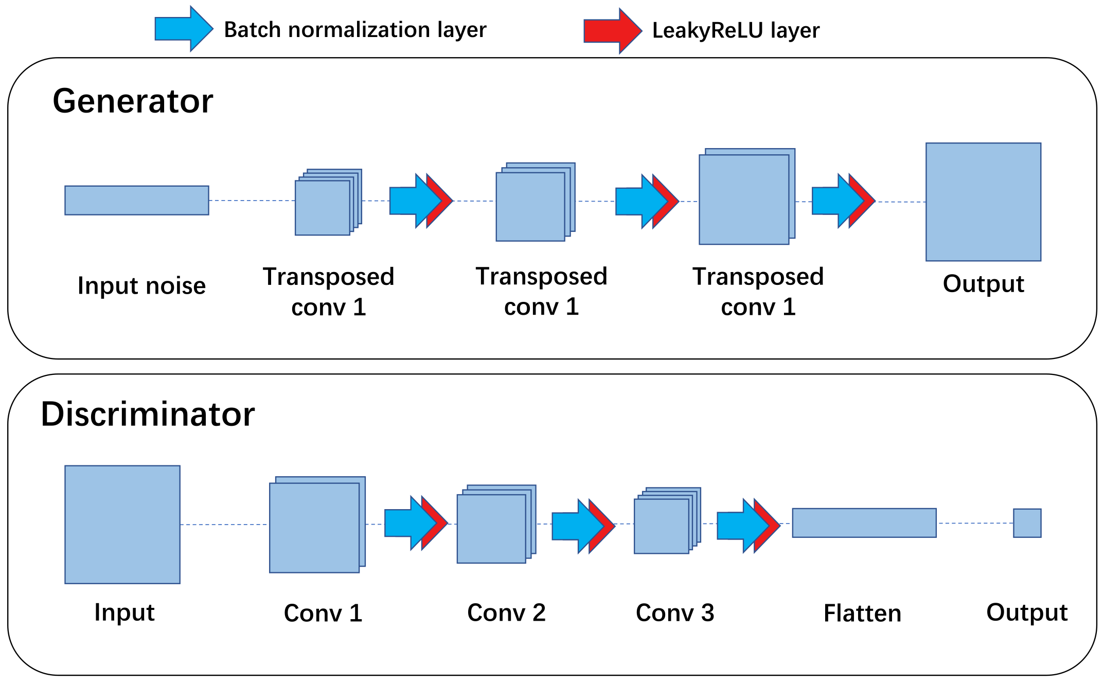
2.1. Theory of the GAN
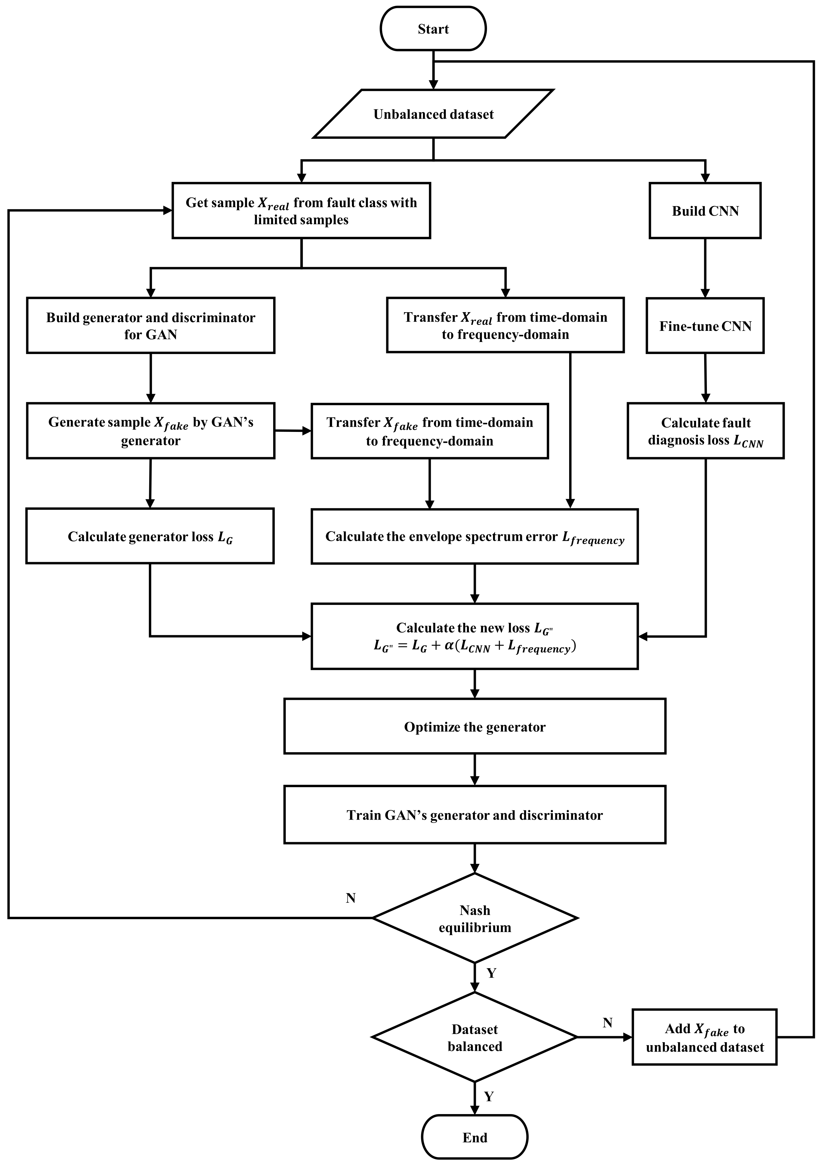
2.2. Fault Data Generation Based on GAN and CNN
2.3. Improvement of Loss Function with Envelope Spectrum
2.4. Collaborative Training Mechanism of the GAN and CNN
3. Experimental dataset
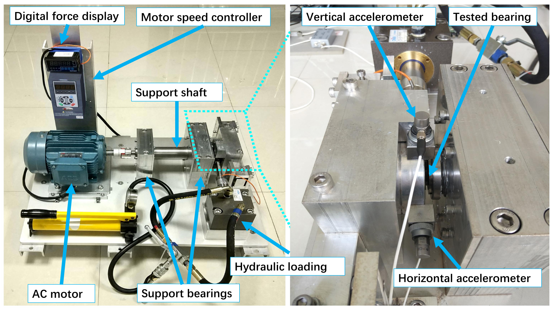
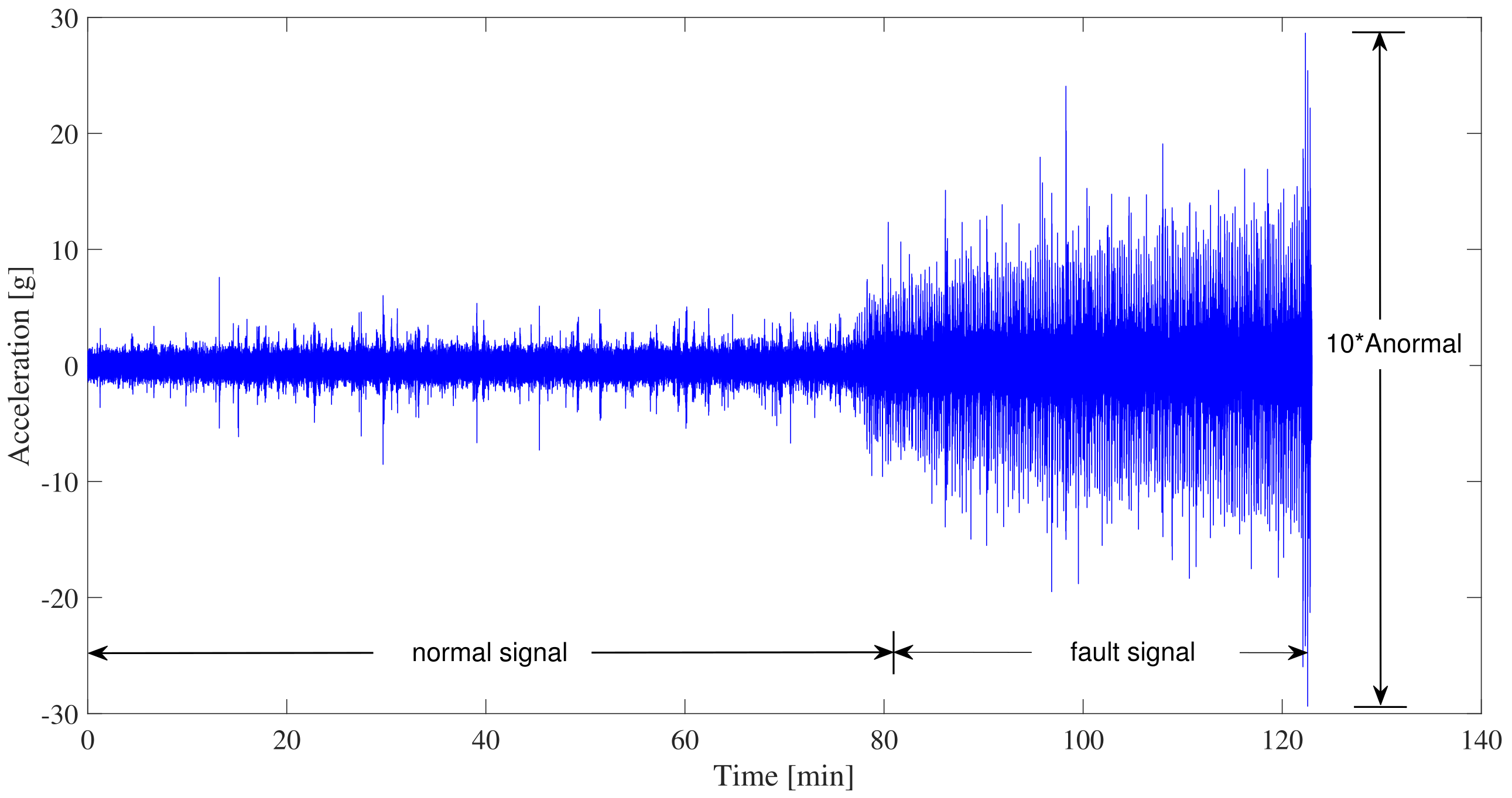
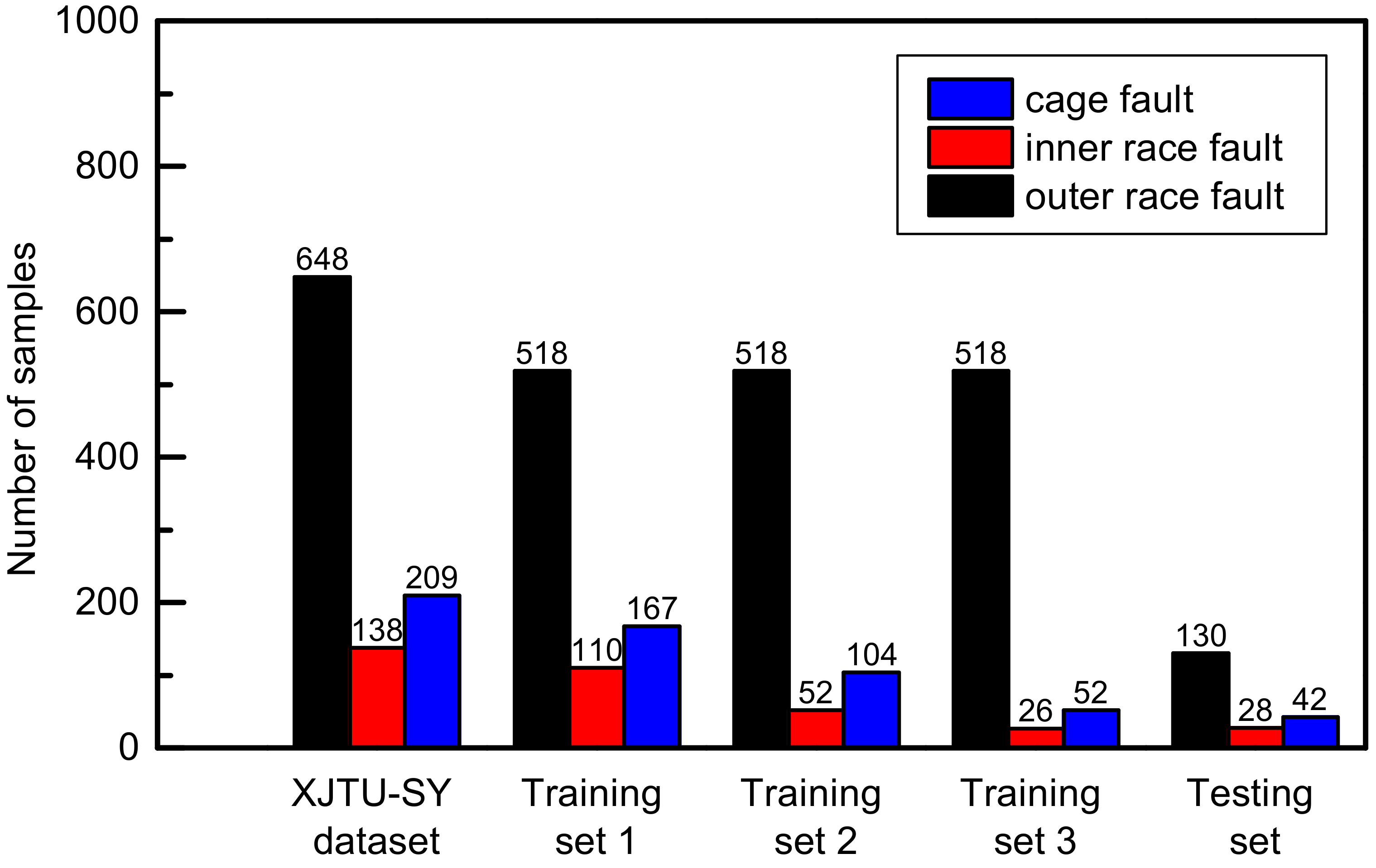
3.1. Introduction of Bearing Test Bench and Dataset
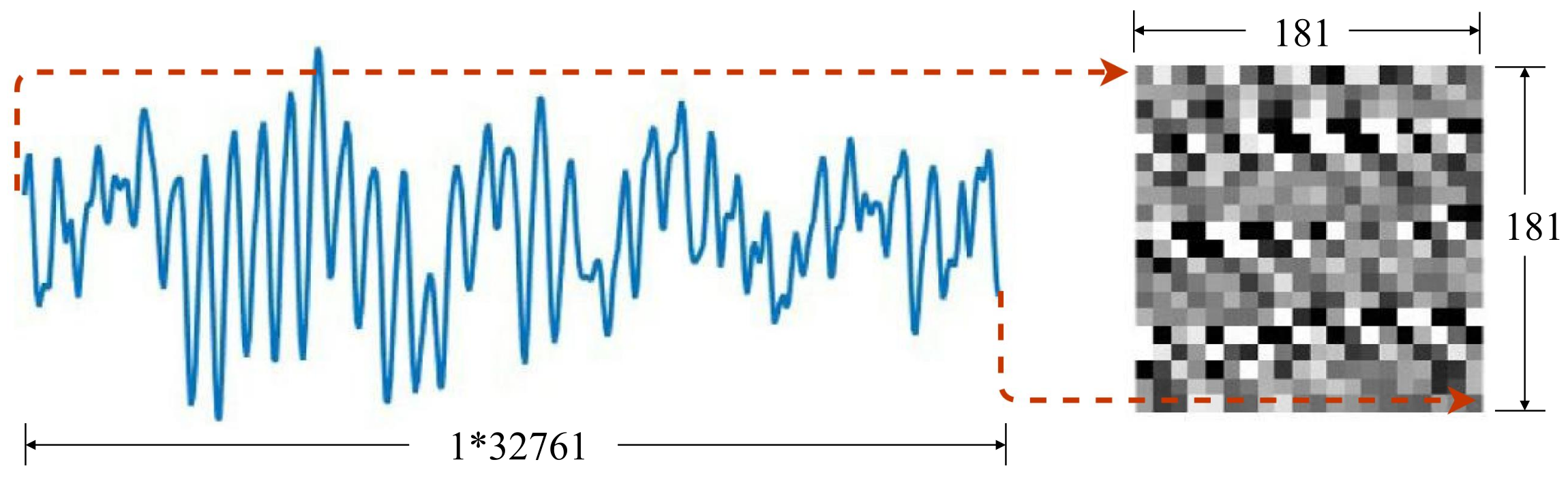
3.2. Data Preprocessing
4. Results and Analysis
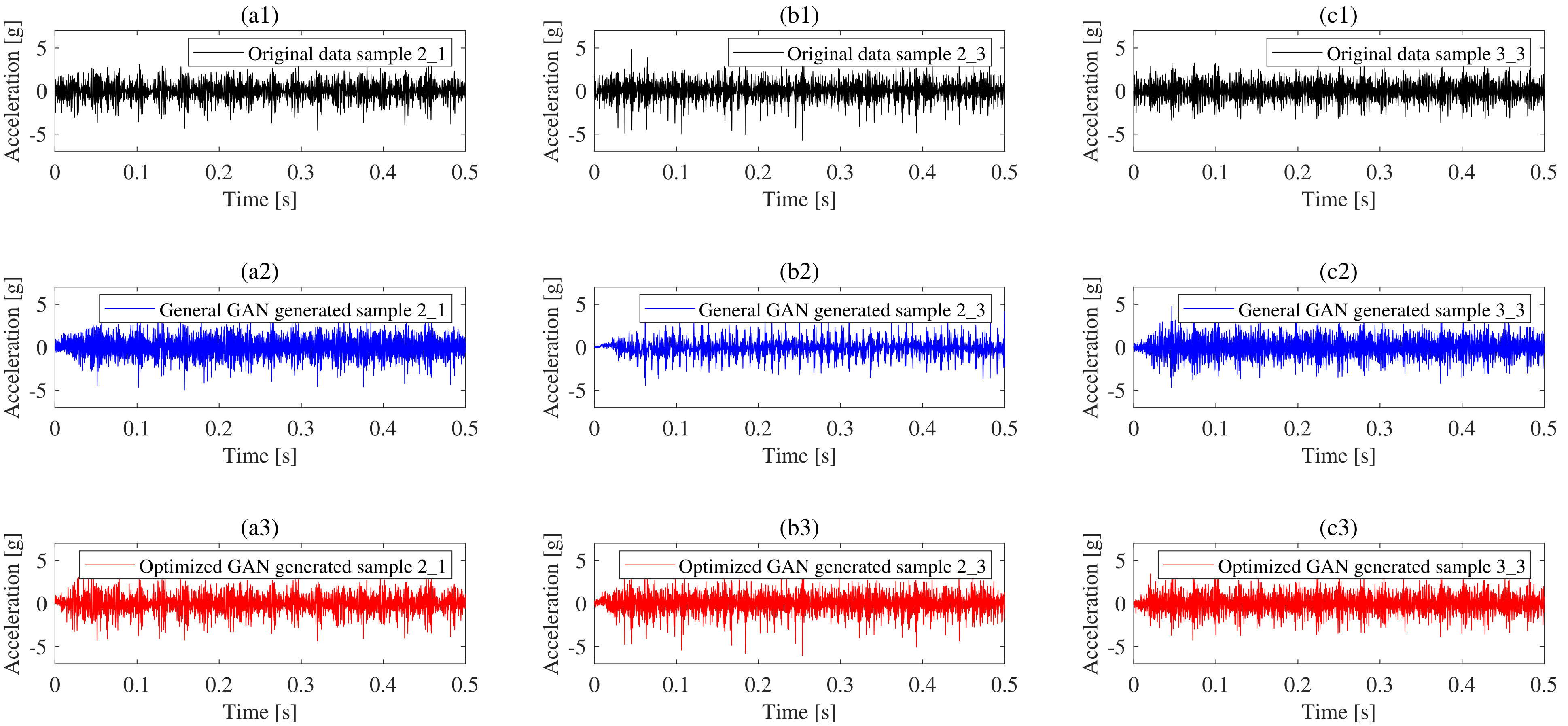
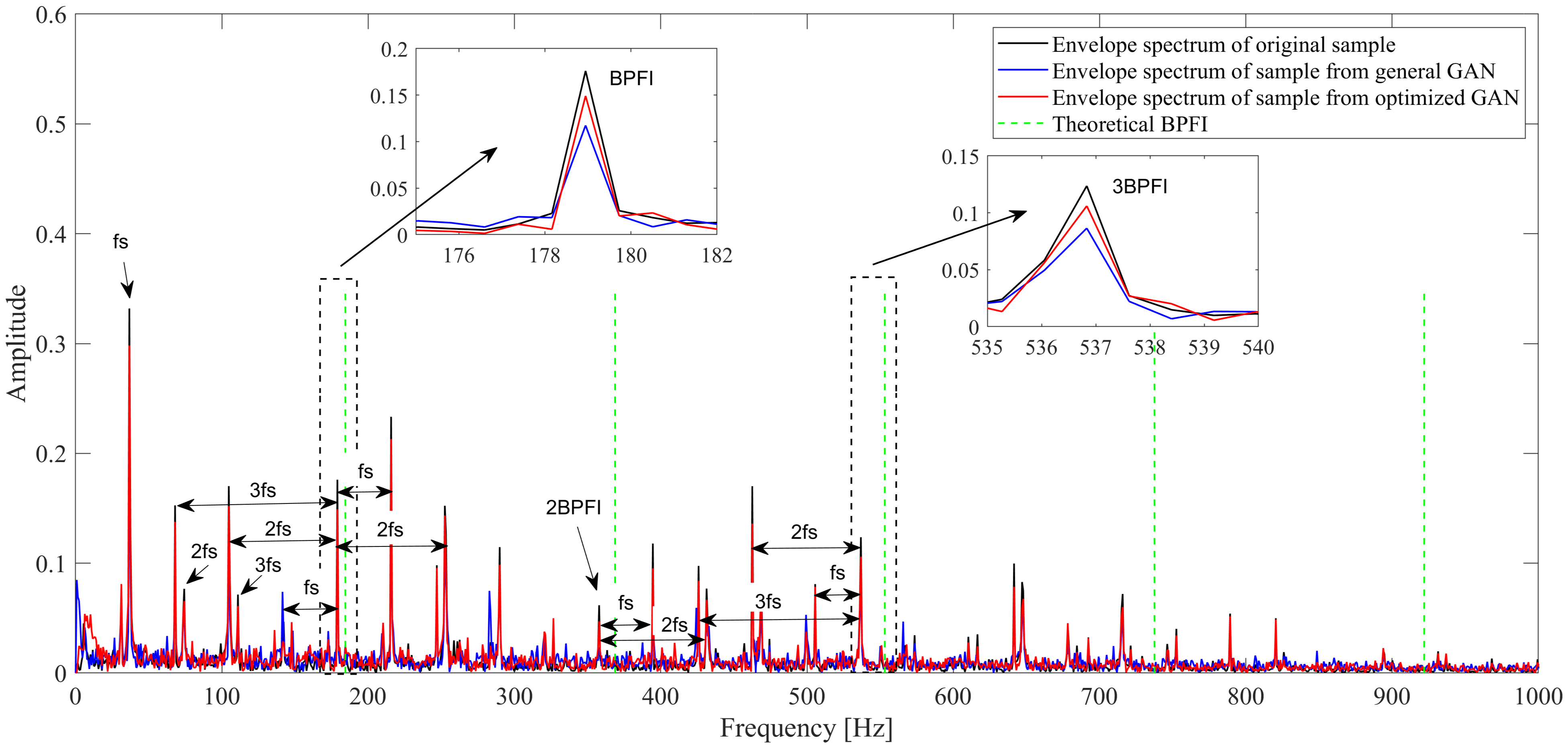
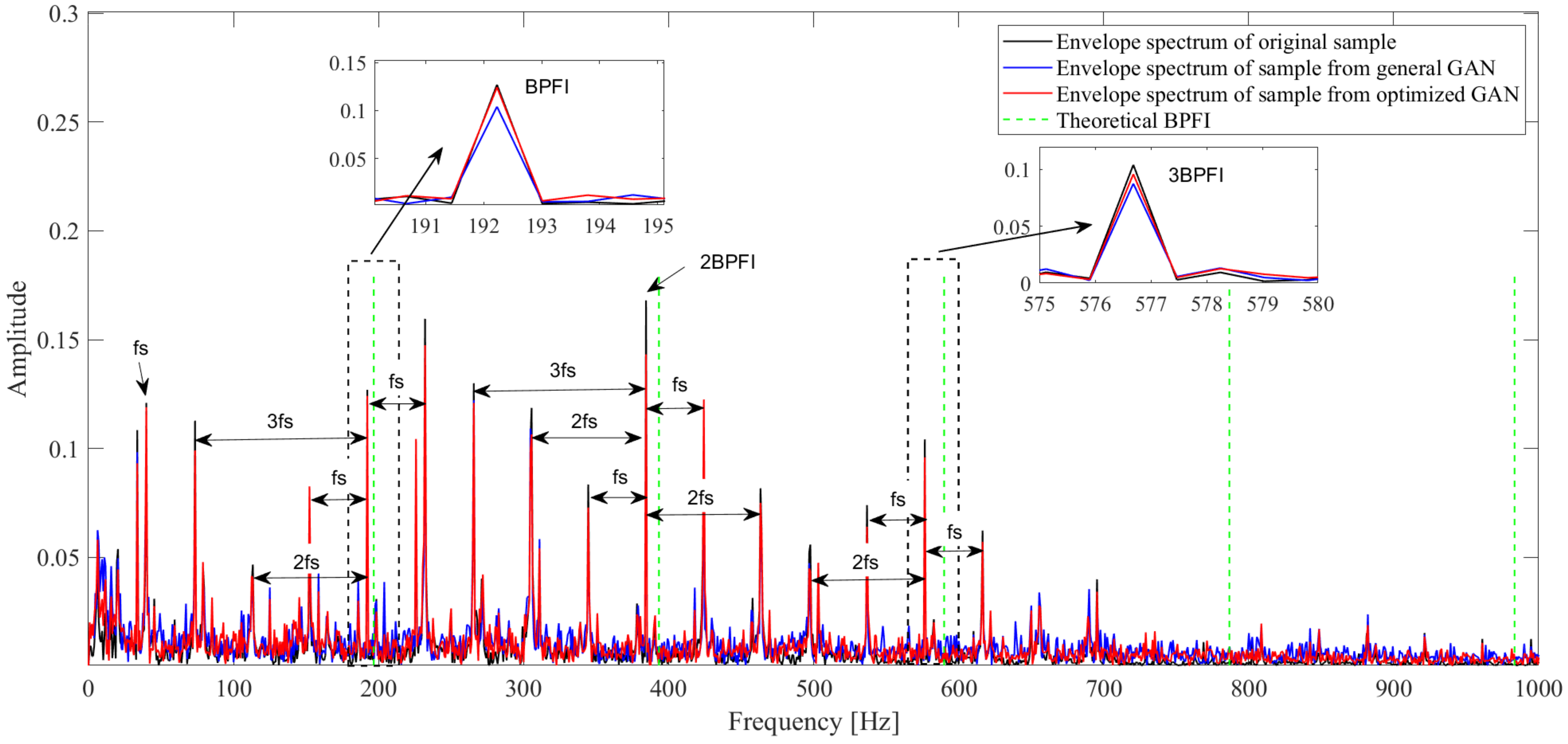
4.1. Fault Data Generation Based on Optimized GAN
4.2. Fault Diagnosis Based on CNN_GAN
5. Conclusions
- A collaborative network GAN_CNN is developed. The GAN generates an almost balanced dataset with data augmentation for the inner ring and the cage fault samples. Once the generated samples are added, the CNN evaluates the extended dataset quality and outputs the fault classification result to modify the loss function of the GAN’s generator.
- Besides the overall similarity, the similarity on the envelope spectrum is considered when building the GAN. The envelope spectrum error from the 1st-5th order between the experimental data and the generated data is taken as a correction term to the general cross-entropy based loss function of the GAN’s generator.
- When constructing the loss function for a GAN, the GAN performance can be improved by considering the envelope spectrum error. The generated samples have higher fidelity and contain more accurate fault information, which, in turn, contribute to the CNN’s accuracy improvement.
- The collaborative network CNN_GAN performs better than the GAN or the CNN. The GAN generates more accurate data if the CNN’s classification results are considered into the GAN’s loss function. The CNN’s fault classification accuracy can be significantly enhanced after the GAN generates more data for the unbalanced training dataset.
Author Contributions
Funding
Institutional Review Board Statement
Informed Consent Statement
Data Availability Statement
Acknowledgments
Conflicts of Interest
Abbreviations
| CNN | Convolutional Neural Networks |
| GAN | Generative Adversarial Networks |
| FCF | Fault characteristic frequency |
| LSTM | Long Short Term Memory |
| BPFO | Ball Passing Frequency on Outer race |
| BPFI | Ball Passing Frequency on Inner race |
| FTF | Fundamental Train Frequency |
References
- Li, N.; Lei, Y.; Lin, J.; Ding, S.X. An improved exponential model for predicting remaining useful life of rolling element bearings. IEEE Trans. Ind. Electron. 2015, 62, 7762–7773. [Google Scholar] [CrossRef]
- Janssens, O.; Slavkovikj, V.; Vervisch, B.; Stockman, K.; Loccufier, M.; Verstockt, S.; Van de Walle, R.; Van Hoecke, S. Convolutional neural network based fault detection for rotating machinery. J. Sound Vib. 2016, 377, 331–345. [Google Scholar] [CrossRef]
- Eren, L.; Ince, T.; Kiranyaz, S. A generic intelligent bearing fault diagnosis system using compact adaptive 1D CNN classifier. J. Signal Process. Syst. 2019, 91, 179–189. [Google Scholar] [CrossRef]
- Zhang, W.; Peng, G.; Li, C. Bearings fault diagnosis based on convolutional neural networks with 2-D representation of vibration signals as input. MATEC Web Conf. 2017, 95, 13001. [Google Scholar] [CrossRef] [Green Version]
- Guo, X.; Chen, L.; Shen, C. Hierarchical adaptive deep convolution neural network and its application to bearing fault diagnosis. Measurement 2016, 93, 490–502. [Google Scholar] [CrossRef]
- Wang, D.; Guo, Q.; Song, Y.; Gao, S.; Li, Y. Application of multiscale learning neural network based on CNN in bearing fault diagnosis. J. Signal Process. Syst. 2019, 91, 1205–1217. [Google Scholar] [CrossRef]
- Sabir, R.; Rosato, D.; Hartmann, S.; Guehmann, C. Lstm based bearing fault diagnosis of electrical machines using motor current signal. In Proceedings of the 18th IEEE International Conference On Machine Learning And Applications (ICMLA), Boca Raton, FL, USA, 16–19 December 2019; pp. 613–618. [Google Scholar]
- Yu, L.; Qu, J.; Gao, F.; Tian, Y. A novel hierarchical algorithm for bearing fault diagnosis based on stacked LSTM. Shock Vib. 2019. [Google Scholar] [CrossRef] [PubMed]
- Qiu, D.; Liu, Z.; Zhou, Y.; Shi, J. Modified Bi-Directional LSTM Neural Networks for Rolling Bearing Fault Diagnosis. In Proceedings of the ICC 2019-IEEE International Conference on Communications (ICC), Shanghai, China, 20–24 May 2019; pp. 1–6. [Google Scholar]
- Pan, H.; He, X.; Tang, S.; Meng, F. An improved bearing fault diagnosis method using one-dimensional CNN and LSTM. J. Mech. Eng 2018, 64, 443–452. [Google Scholar]
- Xiao, D.; Huang, Y.; Qin, C.; Liu, Z.; Li, Y.; Liu, C. Transfer learning with convolutional neural networks for small sample size problem in machinery fault diagnosis. Proc. Inst. Mech. Eng. Part C J. Mech. Eng. Sci. 2019, 233, 5131–5143. [Google Scholar] [CrossRef]
- Zhou, F.; Yang, S.; Fujita, H.; Chen, D.; Wen, C. Deep learning fault diagnosis method based on global optimization GAN for unbalanced data. Knowl.-Based Syst. 2020, 187, 104837. [Google Scholar] [CrossRef]
- Cordón, I.; García, S.; Fernández, A.; Herrera, F. Imbalance: Oversampling algorithms for imbalanced classification in R. Knowl.-Based Syst. 2018, 161, 329–341. [Google Scholar] [CrossRef]
- Ren, S.; Zhu, W.; Liao, B.; Li, Z.; Wang, P.; Li, K.; Chen, M.; Li, Z. Selection-based resampling ensemble algorithm for nonstationary imbalanced stream data learning. Knowl.-Based Syst. 2019, 163, 705–722. [Google Scholar] [CrossRef]
- Shao, S.; Wang, P.; Yan, R. Generative adversarial networks for data augmentation in machine fault diagnosis. Comput. Ind. 2019, 106, 85–93. [Google Scholar] [CrossRef]
- Zhang, W.; Li, X.; Jia, X.D.; Ma, H.; Luo, Z.; Li, X. Machinery fault diagnosis with imbalanced data using deep generative adversarial networks. Measurement 2020, 152, 107377. [Google Scholar] [CrossRef]
- Yuan, B. Efficient hardware architecture of softmax layer in deep neural network. In Proceedings of the 29th IEEE International System-on-Chip Conference (SOCC), Seattle, WA, USA, 6–9 September 2016; pp. 323–326. [Google Scholar]
- Kramer, O. Scikit-learn. In Machine Learning for Evolution Strategies; Springer: Berlin/Heidelberg, Germany, 2016; pp. 45–53. [Google Scholar]
- Wang, B.; Lei, Y.; Li, N.; Li, N. A hybrid prognostics approach for estimating remaining useful life of rolling element bearings. IEEE Trans. Reliab. 2018, 69, 401–412. [Google Scholar] [CrossRef]
- Randall, R.B.; Antoni, J. Rolling element bearing diagnostics—A tutorial. Mech. Syst. Signal Process. 2011, 25, 485–520. [Google Scholar] [CrossRef]
- Niu, L.; Cao, H.; He, Z.; Li, Y. A systematic study of ball passing frequencies based on dynamic modeling of rolling ball bearings with localized surface defects. J. Sound Vib. 2015, 357, 207–232. [Google Scholar] [CrossRef]
- Saruhan, H.; Saridemir, S.; Qicek, A.; Uygur, I. Vibration analysis of rolling element bearings defects. J. Appl. Res. Technol. 2014, 12, 384–395. [Google Scholar] [CrossRef]
- Devogele, T.; Etienne, L.; Esnault, M.; Lardy, F. Optimized discrete fréchet distance between trajectories. In Proceedings of the 6th ACM SIGSPATIAL Workshop on Analytics for Big Geospatial Data, Redondo Beach, CA, USA, 7–10 November 2017; pp. 11–19. [Google Scholar]
- Mishra, C.; Samantaray, A.; Chakraborty, G. Ball bearing defect models: A study of simulated and experimental fault signatures. J. Sound Vib. 2017, 400, 86–112. [Google Scholar] [CrossRef]

| Hyperparameters | Values |
|---|---|
| Initial learning rate of generator | 0.0001 |
| Initial learning rate of discriminator | 0.0001 |
| Kernel size of discriminator’s 1st layer | |
| Kernel size of discriminator’s other layers | |
| Number of filters in discriminator’s n-th layer | |
| Kernel size of generator’s last layer | |
| Kernel size of discriminator’s other layers | |
| Number of filters in generator’s n-th layer | |
| Max epochs | 2000 |
| Hyperparameters | Values |
|---|---|
| Initial learning rate | 0.0002 |
| Max epochs | 1000 |
| Batch size | 20 |
| Kernel size of 1st layer | |
| Kernel size of other layers | |
| Number of filters in n-th layer |
| Parameters | Values | Parameters | Values |
|---|---|---|---|
| Inner raceway diameter | Ball diameter | ||
| Outer raceway diameter | Number of balls | 8 | |
| Pitch diameter | Initial contact angle | 0 |
| Condition | Test Bearing | Measurement Sample Size | Fault Location |
|---|---|---|---|
| (1) = 35 = 12 | bearing 1_1 | 123 | outer ring |
| bearing 1_2 | 161 | outer ring | |
| bearing 1_3 | 158 | outer ring | |
| bearing 1_4 | 122 | cage | |
| bearing 1_5 | 52 | outer ring & inner ring | |
| (2) = = 11 | bearing 2_1 | 491 | inner ring |
| bearing 2_2 | 161 | outer ring | |
| bearing 2_3 | 533 | cage | |
| bearing 2_4 | 42 | outer ring | |
| bearing 2_5 | 339 | outer ring | |
| (3) = 40 = 10 | bearing 3_1 | 2538 | outer ring |
| bearing 3_2 | 2496 | inner ring & element & cage & outer ring | |
| bearing 3_3 | 371 | inner ring | |
| bearing 3_4 | 1515 | inner ring | |
| bearing 3_5 | 114 | outer ring |
| Fault Location | Test Bearing | Measurement Sample Size | Training Sets | Test Sets |
|---|---|---|---|---|
| Outer race | bearing 1_1 | 58 | 518 | 130 |
| bearing 1_2 | 108 | |||
| bearing 1_3 | 69 | |||
| bearing 2_2 | 77 | |||
| bearing 2_4 | 12 | |||
| bearing 2_5 | 173 | |||
| bearing 3_1 | 55 | |||
| bearing 3_5 | 106 | |||
| Inner race | bearing 2_1 | 26 | 110 | 28 |
| bearing 3_3 | 28 | |||
| bearing 3_4 | 84 | |||
| Cage | bearing 1_4 | 1 | 167 | 42 |
| bearing 2_3 | 208 |
| Generated Sample | Cosine Similarity | |
|---|---|---|
| GAN | Optimized GAN | |
| bearing 2_1 | 0.3214 | 0.3739 |
| bearing 3_3 | 0.3374 | 0.3408 |
| bearing 2_3 | 0.2009 | 0.2675 |
| Sample Source | Parameter | 1st— | 2nd— | 3rd— | 4th— | 5th— |
|---|---|---|---|---|---|---|
| Original sample | Frequency (Hz) | 178.944 | 357.889 | 536.833 | 715.788 | 931.449 |
| Amplitude | 0.176 | 0.062 | 0.124 | 0.072 | 0.020 | |
| Sample from general GAN | Frequency (Hz) | 178.944 | 357.889 | 536.833 | 715.788 | 928.323 |
| Error (%) | 0 | 0 | 0 | 0 | 0.34 | |
| Amplitude | 0.117 | 0.023 | 0.086 | 0.053 | 0.011 | |
| Error (%) | 33.3 | 62.0 | 30.1 | 26.1 | 44.1 | |
| Sample from optimized GAN | Frequency | 178.944 | 357.889 | 536.833 | 715.788 | 931.449 |
| Error (%) | 0 | 0 | 0 | 0 | 0 | |
| Amplitude | 0.149 | 0.047 | 0.106 | 0.060 | 0.018 | |
| Error (%) | 15.3 | 23.8 | 14.2 | 16.5 | 9.4 |
| Sample Source | Parameter | 1st— | 2nd— | 3rd— | 4th— | 5th— |
|---|---|---|---|---|---|---|
| Original sample | Frequency (Hz) | 192.229 | 384.457 | 576.686 | 808.767 | 994.744 |
| Amplitude | 0.127 | 0.168 | 0.104 | 0.015 | 0.013 | |
| Sample from general GAN | Frequency (Hz) | 192.229 | 384.457 | 576.686 | 808.767 | 990.055 |
| Error (%) | 0 | 0 | 0 | 0 | 0.5 | |
| Amplitude | 0.104 | 0.131 | 0.088 | 0.019 | 0.006 | |
| Error (%) | 18.0 | 22.1 | 15.9 | 26.0 | 49.5 | |
| Sample from optimized GAN | Frequency (Hz) | 192.229 | 384.457 | 576.686 | 808.767 | 961.143 |
| Error (%) | 0 | 0 | 0 | 0 | 0 | |
| Amplitude | 0.124 | 0.143 | 0.096 | 0.020 | 0.011 | |
| Error (%) | 2.2 | 14.7 | 7.9 | 26.7 | 14.4 |
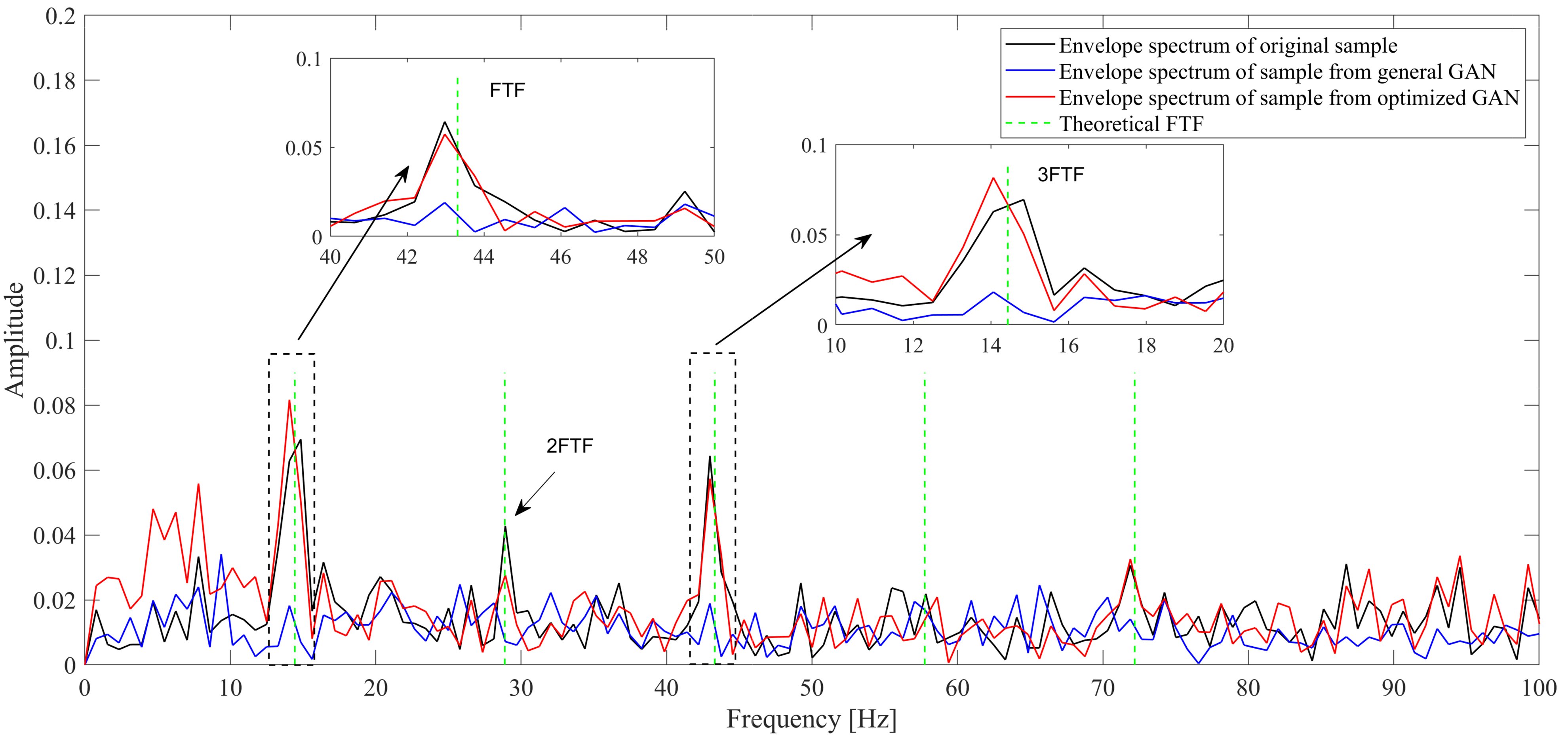
| Sample Source | Parameter | 1st— | 2nd— | 3rd— | 4th— | 5th— |
|---|---|---|---|---|---|---|
| Original sample | Frequency (Hz) | 14.847 | 28.912 | 42.978 | 57.825 | 71.890 |
| Amplitude | 0.069 | 0.043 | 0.064 | 0.022 | 0.031 | |
| Sample from general GAN | Frequency | 14.066 | 28.131 | 42.978 | 57.043 | 71.890 |
| Error (%) | 5.3 | 2.7 | 0 | 1.4 | 0 | |
| Amplitude | 0.018 | 0.019 | 0.019 | 0.020 | 0.014 | |
| Error | 73.3 | 55.4 | 70.6 | 10.7 | 54.1 | |
| Sample from optimized GAN | Frequency (Hz) | 14.066 | 28.912 | 42.978 | 58.606 | 71.890 |
| Error (%) | 5.3 | 0 | 0 | 1.4 | 0 | |
| Amplitude | 0.082 | 0.028 | 0.057 | 0.021 | 0.033 | |
| Error (%) | 17.5 | 35.3 | 10.9 | 4.6 | 6.4 |
| Imbalance Ratio | CNN | CNN_GAN | ||
|---|---|---|---|---|
| Accuracy | Cross-Entropy Error | Accuracy | Cross-Entropy Error | |
| Training set 1 (5:1:1.5) | 98% | 0.6071 | 100% | 0.5645 |
| Training set 2 (10:1:2) | 88% | 0.7013 | 90% | 0.6642 |
| Training set 3 (20:1:2) | 68% | 0.8478 | 88% | 0.7012 |
| Diagnosis Network | Confusion Matrix on Testing Set | ||
|---|---|---|---|
| Training with Set 1 Unbalance Ratio (5:1:1.5) | Training with Set 2 Unbalance Ratio (10:1:2) | Training with Set 3 Unbalance Ratio (20:1:2) | |
| CNN |  | 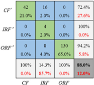 | 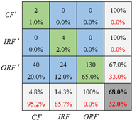 |
| CNN_GAN |  |  | 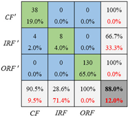 |
Publisher’s Note: MDPI stays neutral with regard to jurisdictional claims in published maps and institutional affiliations. |
© 2021 by the authors. Licensee MDPI, Basel, Switzerland. This article is an open access article distributed under the terms and conditions of the Creative Commons Attribution (CC BY) license (https://creativecommons.org/licenses/by/4.0/).
Share and Cite
Ruan, D.; Song, X.; Gühmann, C.; Yan, J. Collaborative Optimization of CNN and GAN for Bearing Fault Diagnosis under Unbalanced Datasets. Lubricants 2021, 9, 105. https://doi.org/10.3390/lubricants9100105
Ruan D, Song X, Gühmann C, Yan J. Collaborative Optimization of CNN and GAN for Bearing Fault Diagnosis under Unbalanced Datasets. Lubricants. 2021; 9(10):105. https://doi.org/10.3390/lubricants9100105
Chicago/Turabian StyleRuan, Diwang, Xinzhou Song, Clemens Gühmann, and Jianping Yan. 2021. "Collaborative Optimization of CNN and GAN for Bearing Fault Diagnosis under Unbalanced Datasets" Lubricants 9, no. 10: 105. https://doi.org/10.3390/lubricants9100105
APA StyleRuan, D., Song, X., Gühmann, C., & Yan, J. (2021). Collaborative Optimization of CNN and GAN for Bearing Fault Diagnosis under Unbalanced Datasets. Lubricants, 9(10), 105. https://doi.org/10.3390/lubricants9100105