Article

Collaborative Optimization of CNN and GAN for Bearing Fault Diagnosis under Unbalanced Datasets

1
Chair of Electronic Measurement and Diagnostic Technology, Technische Universität Berlin, 10587 Berlin, Germany
2
School of Electrical Engineering and Computer Science, Technische Universität Berlin, 10587 Berlin, Germany
3
School of Vehicle and Mobility, Tsinghua University, Beijing 100084, China
*
Author to whom correspondence should be addressed.
Lubricants 2021, 9(10), 105; https://doi.org/10.3390/lubricants9100105
Submission received: 23 August 2021 / Revised: 6 October 2021 / Accepted: 8 October 2021 / Published: 15 October 2021
(This article belongs to the Special Issue Machine Learning in Tribology)

Abstract

:
Convolutional Neural Network (CNN) has been widely used in bearing fault diagnosis in recent years, and many satisfying results have been reported. However, when the training dataset provided is unbalanced, such as the samples in some fault labels are very limited, the CNN’s performance reduces inevitably. To solve the dataset imbalance problem, a Generative Adversarial Network (GAN) has been preferably adopted for the data generation. In published research studies, GAN only focuses on the overall similarity of generated data to the original measurement. The similarity in the fault characteristics is ignored, which carries more information for the fault diagnosis. To bridge this gap, this paper proposes two modifications for the general GAN. Firstly, a CNN, together with a GAN, and two networks are optimized collaboratively. The GAN provides a more balanced dataset for the CNN, and the CNN outputs the fault diagnosis result as a correction term in the GAN generator’s loss function to improve the GAN’s performance. Secondly, the similarity of the envelope spectrum between the generated data and the original measurement is considered. The envelope spectrum error from the 1st to 5th order of the Fault Characteristic Frequencies (FCF) is taken as another correction in the GAN generator’s loss function. Experimental results show that the bearing fault samples generated by the optimized GAN contain more fault information than the samples produced by the general GAN. Furthermore, after the data augmentation for the unbalanced training sets, the CNN’s accuracy in the fault classification has been significantly improved.

1. Introduction

As an indispensable component in rotating machines, bearing health status directly affects or even determines the equipment service life. However, in practice, a bearing usually works under extreme and harsh conditions, which makes the bearing prone to faults [1]. Therefore, the timely and accurate fault diagnosis is crucial to reduce the maintenance costs and avoid serious accidents.
In recent years, the data-driven fault diagnosis has been attracting more and more attention from both academia and industry. Among the various data-driven methods, Convolution Neural Network (CNN) and Long Short Term Memory (LSTM) are the most widely used due to their powerful abilities in the complex feature extraction and nonlinear mapping. CNN was first employed in the bearing fault diagnosis by O. Janssens in 2016 [2], and, since then, many improvements have proposed to enhance the CNN’s performance, such as 1D-CNN, 2D-CNN, multiscale CNN, and adaptive CNN [3,4,5,6]. Russell Sabir adopted LSTM for the bearing fault diagnosis based on the motor current signal and obtained a classification accuracy of 96% [7]. L. Yu and D. Qiu proposed the stacked LSTM and the bidirectional LSTM, respectively, and both LSTMs obtained an accuracy of more than 99% on the bearing fault diagnosis [8,9]. H. Pan combined 1D-CNN and 1D-LSTM into a unified structure by using the CNN’s output into LSTM, achieving a satisfactory test accuracy up to 99.6% [10].
Although many sound results have been reported in the deep learning-based fault diagnosis, there are still many challenges to be solved. For example, all the studies mentioned above assume that there are plenty of high quality data for the deep network training. However, in many applications, the available history or experimental data is very limited or data provided is severely unbalanced. For example, the sample size under some fault classes is extremely smaller compared with the others. Either insufficient or unbalanced data will cause the serious performance reduction of deep networks. According to D. Xiao’s work, when the training set samples were reduced from 1000 to 150, the CNN’s accuracy declined correspondingly from 97.2% to 83.9% [11]. When the imbalance ratio increased from 2:1 to 40:1, the fault classification accuracy for the outer ring fault based on the GAN-SAE dropped sharply from 97.79% to 20.95% [12].
To address this problem, scholars have proposed diverse methods. Oversampling was first proposed to solve the data imbalance, where the direct replication was used to generate more samples for such labels that had very few ones [13,14]. Although this method is simple and efficient, it easily causes overfitting since no new information is incorporated. As another prospective method for data generation, GAN has been already used for new sample generation in the fault diagnosis. Both W. Zhang and S. Shao employed GAN to learn the mapping between the noise distribution and the actual machinery vibration data to expand available dataset. The results confirmed that the diagnosis accuracy could be improved once the imbalanced data was augmented by GAN [15,16]. However, when building and evaluating the GAN, published research studies only focus on the overall similarity between the generated data and the original one, which inevitably brings problems in the data quality. Small loss function in the general GAN only means that the generated data has a high similarity to the original signal, but it does not guarantee that the generated signal has captured the important characteristics of the original signal. When generating more samples for the unbalanced datasets in the fault diagnosis, it is important to ensure that the generated sample carries the same or nearly the same fault information as the original one, which includes both time and frequency domain characteristics. For this reason, an improved GAN is proposed in this paper and applied to generate samples for an unbalanced experimental dataset which is further used in the CNN-based fault diagnosis.
The main innovations of this paper include: (1) A GAN, together with a CNN, and two networks are optimized in cooperation. The GAN generates a more balanced dataset for the CNN, and the CNN evaluates the quality of the GAN’s data generation. Both networks contribute to each other in performance improvement. (2) The fault characterization information is used to improve the general entropy-based loss function in the GAN. The amplitude and frequency errors in the envelope spectrum between the experimental and generated samples are taken as a correction term in the GAN’s loss function to enable the GAN to produce samples with higher fidelity and identify more fault information.
The remaining part of this paper is organized as follows. Section 2 details the theory and methodology of the GAN, CNN, and loss function improvement. Section 3 describes the test bench and experimental dataset. Section 4 discusses and analyzes the results. Section 5 concludes the whole paper.

2. Methodology

2.1. Theory of the GAN

A GAN generates new data without any prior knowledge of the probability density function of original data. It mainly consists of a generator and a discriminator. The discriminator determines whether a sample comes from the original or generated dataset. On the contrary, the generator tries to produce data similar to the original one so that the discriminator can hardly make right decisions. In the general GAN, the loss functions of generator and discriminator are defined as Equations (1) and (2), respectively [15]:
L G = 1 K i = 1 K log D x f a k e i ,
L D = 1 J m = 1 J log D x r e a l m 1 K i = 1 K log 1 D x f a k e i ,
where J is the number of real samples, and K is the number of generated samples. x r e a l m represents the data samples coming from the real training dataset, and x f a k e i denotes the data samples from GAN generator. D ( x r e a l m ) designates the output of discriminator D with the input data sample x r e a l m .
Based on the loss function L G and L D , the GAN can be trained as a minmax two-player game until the global optimum, D ( x r e a l ) = D ( x f a k e ) = 0.5 , is reached. This indicates that the generated data from the generator is so similar to the real one that the discriminator cannot tell the difference.

2.2. Fault Data Generation Based on GAN and CNN

The direct task of a GAN is to generate more samples for the labels with limited measurements. However, the ultimate goal is to improve the data-driven fault-diagnosis method performance when it deals with the imbalanced datasets. Therefore, it is reasonable to take the final fault-diagnosis results into consideration when constructing a GAN so that the data generated can indeed sharpen the algorithm’s fault-diagnosis ability. In this paper, to facilitate research, a CNN is selected as a representative of the data-driven fault-diagnosis methods, and the diagnosis task is focused on the fault classification, so its performance is evaluated by the cross-entropy, as shown in Equation (3). The CNN’s result is introduced as a correction term in the GAN’s generator loss function as formulated in Equation (4):
L C N N = i = 1 N x i log p i ,
L G = L G + β L C N N ,
where N is the number of bearing fault types. x i = 1 , if the input sample belongs to the bearing fault type i; otherwise, x i = 0 . p i is the output of softmax function, which represents the probability that the input data belongs to the bearing fault type i. The formulation for p i is given in Equation (5), and it satisfies i = 1 N p i = 1 [17]. β is a scale factor to keep the loss functions of the GAN and CNN at the same range.
p i = e a i i = 1 N e a i .

2.3. Improvement of Loss Function with Envelope Spectrum

The general GAN can produce data with high similarity to the original measurement, as stated in the last sub-section. In theory, the data fidelity can be even improved when a CNN is employed to collaboratively optimize a GAN. However, until now, all the data points in a sample are treated equally, and the GAN’s target is to keep the generated data as similar to the original one as possible. However, in the fault diagnosis, some data points contain more information than others. For example, once a fault occurs on a certain component, such as the outer and inner ring or the balls, the corresponding fault characteristic frequencies ( F C F ) will appear in the acceleration spectrum. Compared with the overall similarity, the frequency and amplitude at the fault characteristic frequencies contain much more information about the bearing health condition. Therefore, the error of amplitudes and frequencies between the original signal and the generated one at the fault characteristic frequencies is defined as another correction term in the frequency domain as follows:
L f r e q u e n c y = i = 1 N M r e a l i M f a k e i + F r e a l i F f a k e i ,
where N denotes the maximum order of F C F , and N = 5 in this study. M r e a l i and M f a k e i stand for the i-th order F C F amplitude from the real and generated sample. F r e a l i and F f a k e i represent the i-th order F C F frequency from the real and generated sample. In addition, due to different value ranges of frequency and amplitude, in this study, the most widely used normalization method, MinMaxScaler [18], is applied to normalize the amplitudes and frequencies within the 5th-order F C F to the range of [0, 1].
Finally, L f r e q u e n c y is combined with L C N N to construct the final loss function of the GAN’s generator. As shown in Equation (7), the sum of L C N N and L f r e q u e n c y is taken as a modification term in the general GAN’s loss function L G to ensure the generated data from GAN has a high similarity and captures the important information in detail at the same time. α is a weight factor.
L G = L G + α L C N N + L f r e q u e n c y .
To obtain L f r e q u e n c y , the first step is to calculate the theoretical F C F . The XJTU-SY dataset [19] introduced in the following section includes only three kinds of faults, namely the outer race fault, the inner race fault, and the cage fault. The theoretical F C F s for the aforementioned 3 fault types are the B P F O (Ball Passing Frequency on Outer race), B P F I (Ball Passing Frequency on Inner race), and F T F (Fundamental Train Frequency), respectively. Their formulations are listed as follows [20]:
B P F O = n f s 2 1 d D cos α ,
B P F I = n f s 2 1 + d D cos α ,
F T F = f s 2 1 d D cos α ,
where n is the number of rolling elements, and f s means the shaft frequency. d represents the ball diameter, and D denotes the pitch diameter. α is the bearing contact angle.
After calculation of the theoretical F C F , the second step is to capture the actual F C F around corresponding theoretical values. The actual F C F can be affected by many factors, such as the shaft speed, external load, friction coefficient, raceway groove curvature, and the defect size [21,22]. Therefore, there exists bias between the theoretical F C F and the actual F C F in most cases. Besides, some harmonics of F C F influenced by modulation of other vibrations may not be detected in the test bench [22]. Thus, in this paper, the i-th order actual F C F is determined as the maximum peak in the interval of 0.95 , 1.05 × F C F 1 s t × i , where F C F 1 s t is the first order theoretical F C F , and i is the current frequency order. The actual F C F of both the real measurement sample and generated sample are determined by above two steps. Once actual F C F is identified, the L f r e q u e n c y can be obtained by Equation (6).

2.4. Collaborative Training Mechanism of the GAN and CNN

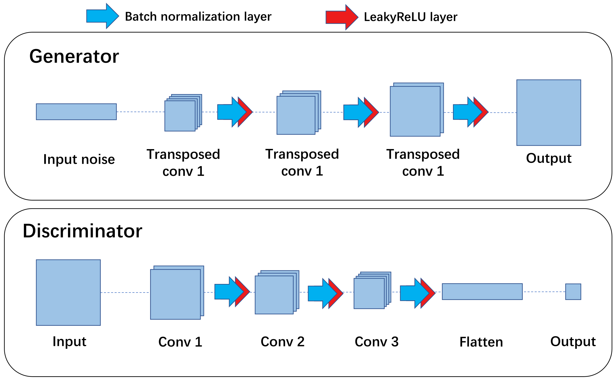
Once the modification for the GAN loss function has been determined, the next step is to train a GAN in cooperation with a CNN. The collaborative training process is demonstrated in Figure 1. Generally, a GAN provides a more balanced dataset for CNN to improve its fault diagnosis accuracy. Whereas CNN evaluates the GAN’s generated dataset and outputs its fault classification result as a correction term in the generator’s loss function to improve the GAN’s data-generation quality, under the collaborative training structure, both CNN and GAN performance can be enhanced. Specifically, as shown in Figure 1, the CNN is firstly built based on the unbalanced dataset, and its classification error is supposed to be high. Meanwhile, the discriminator, as well as the generator, of the GAN are established. Initially, the generator does not work so well, and the generated samples are not so similar to the original ones. The next step is to optimize the CNN and GAN collaboratively. During the optimization process, the GAN’s generator learns to generate samples similar to the original signal. The newly generated samples are immediately added to the training dataset of the CNN so that the dataset imbalance can be reduced. When the Nash equilibrium is reached, which is defined as D ( x r e a l ) = D ( x f a k e ) = 0.5 , the optimization process stops. Lastly, the GAN’s generator is used to extend the original dataset and fine-tune the CNN with the extended dataset. The architecture of the GAN proposed in this paper is detailed in Figure 2. Table 1 and Table 2 summarize the hyperparameters of the GAN and CNN, respectively.

3. Experimental dataset

3.1. Introduction of Bearing Test Bench and Dataset

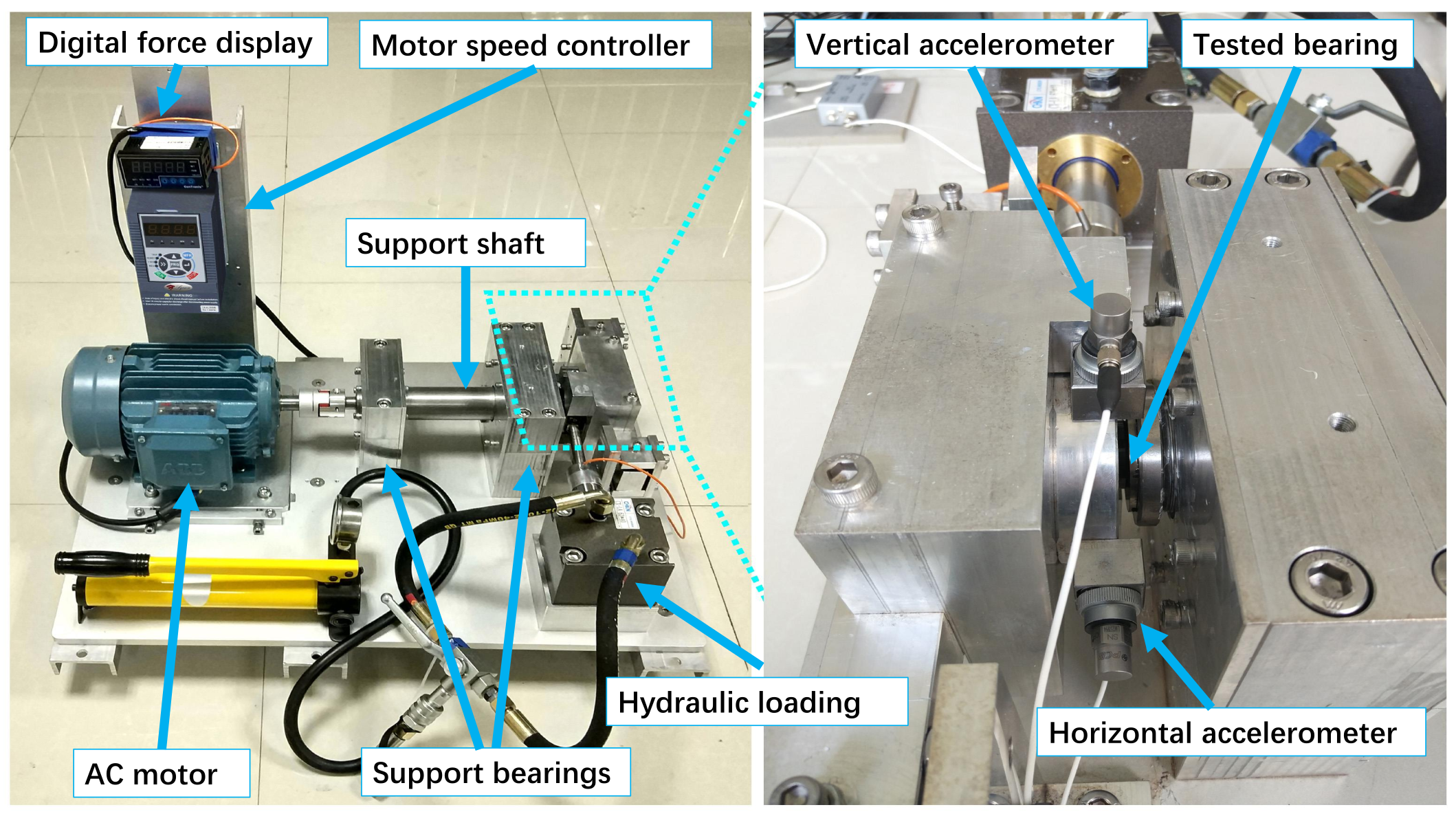
Experimental data for validation comes from the Xi’an Jiaotong University (XJTU-SY) bearing test bench [19]. As shown in Figure 3, the bearing accelerated life test bench consists of an alternating current induction motor, motor speed controller, supporting shaft, supporting bearing, hydraulic loading system, and test bearing. The test bearing type is LDK UER204, and its basic parameters are summarized in Table 3. The bearing works under 3 different conditions, as specified in the first column of Table 4, where f s stands for the shaft frequency, and F r the radial loading force. Both the axial and radial accelerations are measured at a sampling frequency of 25.6   k Hz , and the sampling interval between any two measurements is defined as 1 min , and each sampling lasts for 1.28   s . Under each condition, 5 bearings are tested, such as bearing 1_1–1_5 under condition 1. As each test bearing has a different lifetime, the measurement sample size of each test bearing varies from one to another.
Due to the inherent micro-anisotropy and different working conditions, the lifetime and failure location of the test bearing differ from each other. For a single fault, there are 3 fault types in total, namely the outer race fault, the inner race fault, and the cage fault. Moreover, there are two datasets, bearing 1_5 and bearing 3_2, containing the measurements of compound fault. To simplify the labeling process, only a single fault is considered in this paper. As summarized in Table 4, the number of total samples is large enough for CNN training. However, the dataset is extremely unbalanced. For the most test bearings under all 3 conditions, the failure occurs on the outer ring, with very limited samples on the inner ring and the cage.

3.2. Data Preprocessing

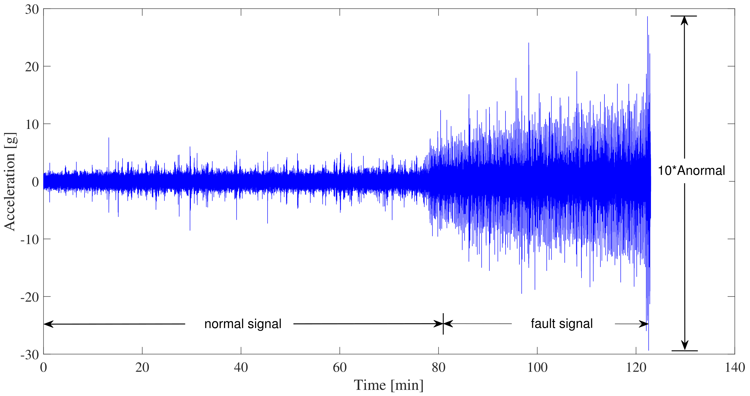
The XJTU-SY bearing dataset has recorded the bearing acceleration during the whole life cycle. The test bench runs continuously until the acceleration amplitude exceeds 10 × A n o r m a l , which is defined as the failure point. Here, A n o r m a l is the maximum amplitude of the horizontal or vertical vibration signals when the bearing runs in the normal operating stage. The fault location in Table 4 stands for position where the fault happens when bearing finally fails. In order to extract the sufficient measurement data for the fault classification while maintaining the correct labels, the signals with acceleration amplitude between 2 × A n o r m a l and 10 × A n o r m a l are regarded as the fault signals, as shown in Figure 4. All the measurement samples in the fault period are labeled with the corresponding final failure position, such as 1 for the cage fault, 2 for the inner race fault, and 3 for the outer race fault.
After preparation for the valid source data and labels, the next step is the data preprocessing. At first, the original measurement is denoised by 3-level wavelet decomposition, with S y m l e t 4 as the mother wavelet. After the noise cancellation for the high-frequency components, the data is normalized by z-score. Finally, the normalized data is transformed from 1D to 2D, which means that the acceleration series are sliced into fragments with the same length and then stacked row by row to build a matrix, as illustrated in Figure 5. In each sample, there are a total of 32,768 points of data in each sample. Therefore, the size of 2D matrix is determined as 181 × 181 , and the reshaped 2D matrix is fed into GAN and CNN as images. All the work in this study is conducted in MATLAB Deep Network Designer.

4. Results and Analysis

4.1. Fault Data Generation Based on Optimized GAN

According to Table 5, there are significantly more samples for the outer race fault than for the inner race fault and the cage fault. Consequently, generating more samples for the inner race fault and the cage fault is paramount to reduce the dataset imbalance. It should be noticed that the inner race fault samples consist of data from bearing 2_1, bearing 3_3, and bearing 3_4, while the cage fault samples consist of data from bearing 1_4 and bearing 2_3. This means both the inner race and cage faults have measurement samples collected from different working conditions that define different data distributions. Furthermore, each test bearing has totally different aging dynamics, which can be deduced from their full life cycle trajectories [19]. As a result, the GANs for these datasets need to be trained individually. Bearing 1_4 has only one sample and is, hence, not feasible for the fault diagnosis. In total, 4 GANs need to be established for bearing 2_1, bearing 2_3, bearing 3_3, and bearing 3_4.
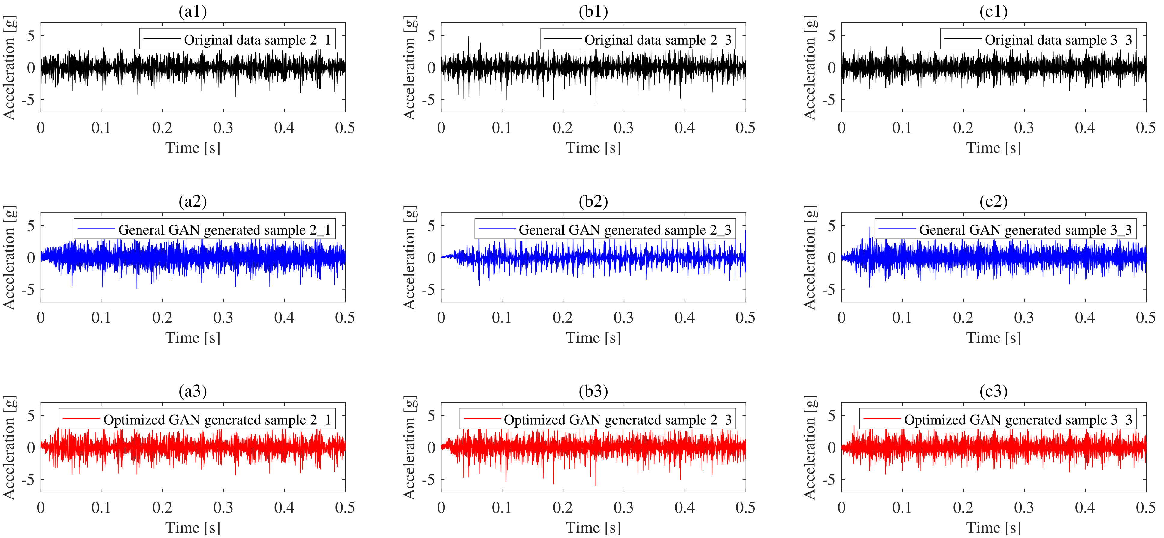
The data samples generated by a general GAN and an optimized GAN are illustrated in Figure 6 and compared with the original ones after normalization. Specifically, Figure 6(a1) stands for the original signal of a measurement sample from bearing 2_1, Figure 6(a2) is the corresponding sample generated by the general GAN, and Figure 6(a3) shows the sample generated by the optimized GAN. Likewise, Figure 6(b1–b3) are the result for bearing sample 2_3, and Figure 6(c1–c3) for bearing sample 3_3. Take the inner race fault bearing 2_1 as an example; both GANs produce the samples with high similarity to the original ones measured in time domain, and even the peaks are accurately rebuilt. It can be further noticed that the optimized GAN generates a much more accurate peak amplitude than the general GAN. In order to evaluate the GAN’s data-generation quality in time domain, every sample is regarded as a vector x ( x R D ), and every sampling point x i as an element in the vector.
The similarity between the generated sample and the original one can be measured by the angle between two corresponding vectors. Therefore, cosine similarity is adopted as a time domain similarity metric, which is defined as follows:
cos θ = m · n | m | · | n | ,
where m and n stand for the acceleration series from the original measurement and the generated sample, respectively, with m = x 1 , x 2 , , x L and n = x 1 , x 2 , , x L . | m | and | n | identify the 2-norm of m and n , respectively.
The cosine similarity results are summarized in Table 6. For all 3 cases, the sample generated by the optimized GAN has higher cosine similarity to the original one than that produced by the general GAN, which proves the superiority of the optimized GAN in the high-quality data generation. Additionally, the reason why the cosine similarity is relatively small can be explained as the acceleration values change within a big range of [ 5 , 5 ] , and the signal length is up to 32,761, which means any difference in acceleration amplitude or direction or time lag between counterpart points will bring big accumulative deviation. Besides, the assumption by taking the acceleration signal as 1D vector may not be so feasible when it contains too many elements, which needs further exploration in the future, such as using the Fréchet distance to replace the cosine similarity [23].
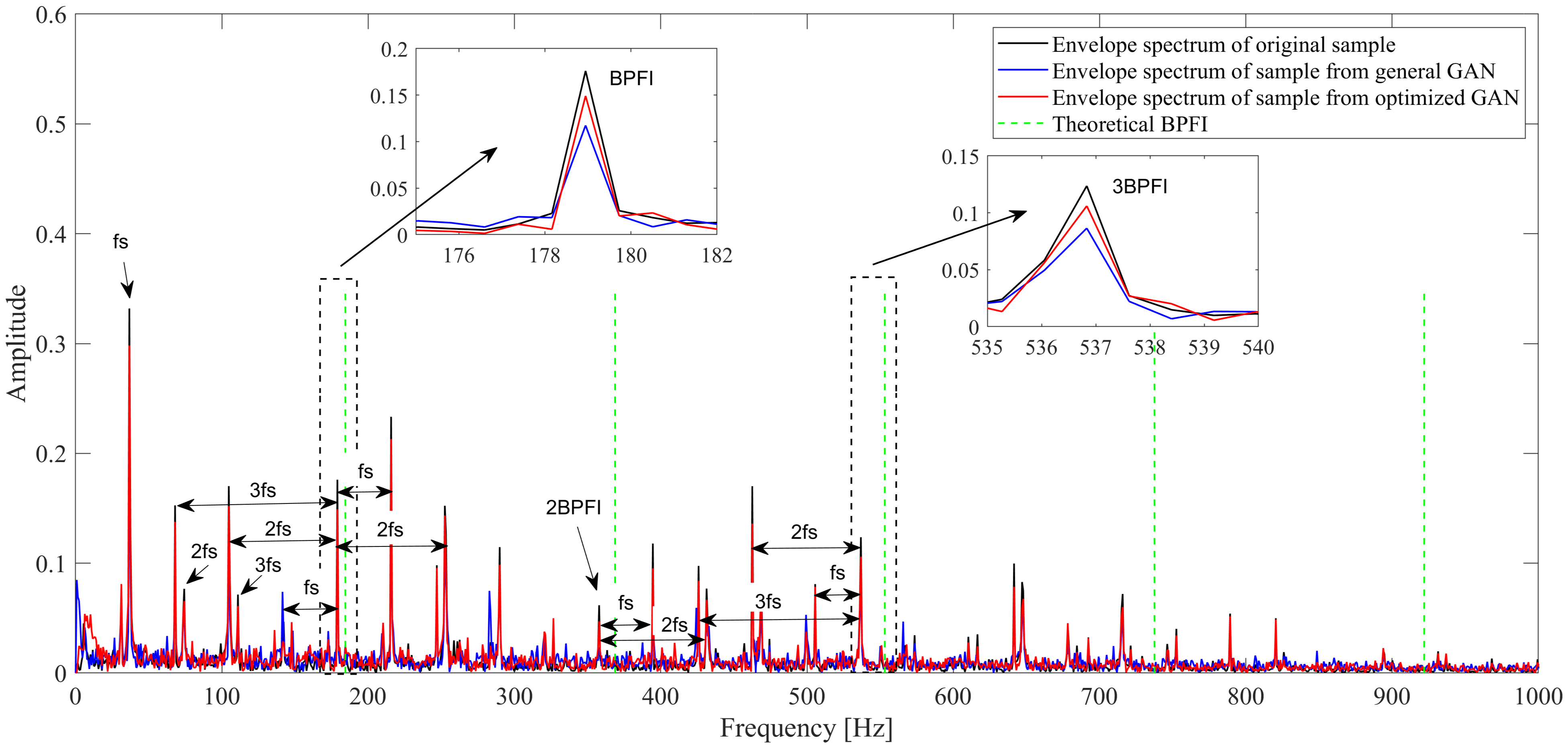
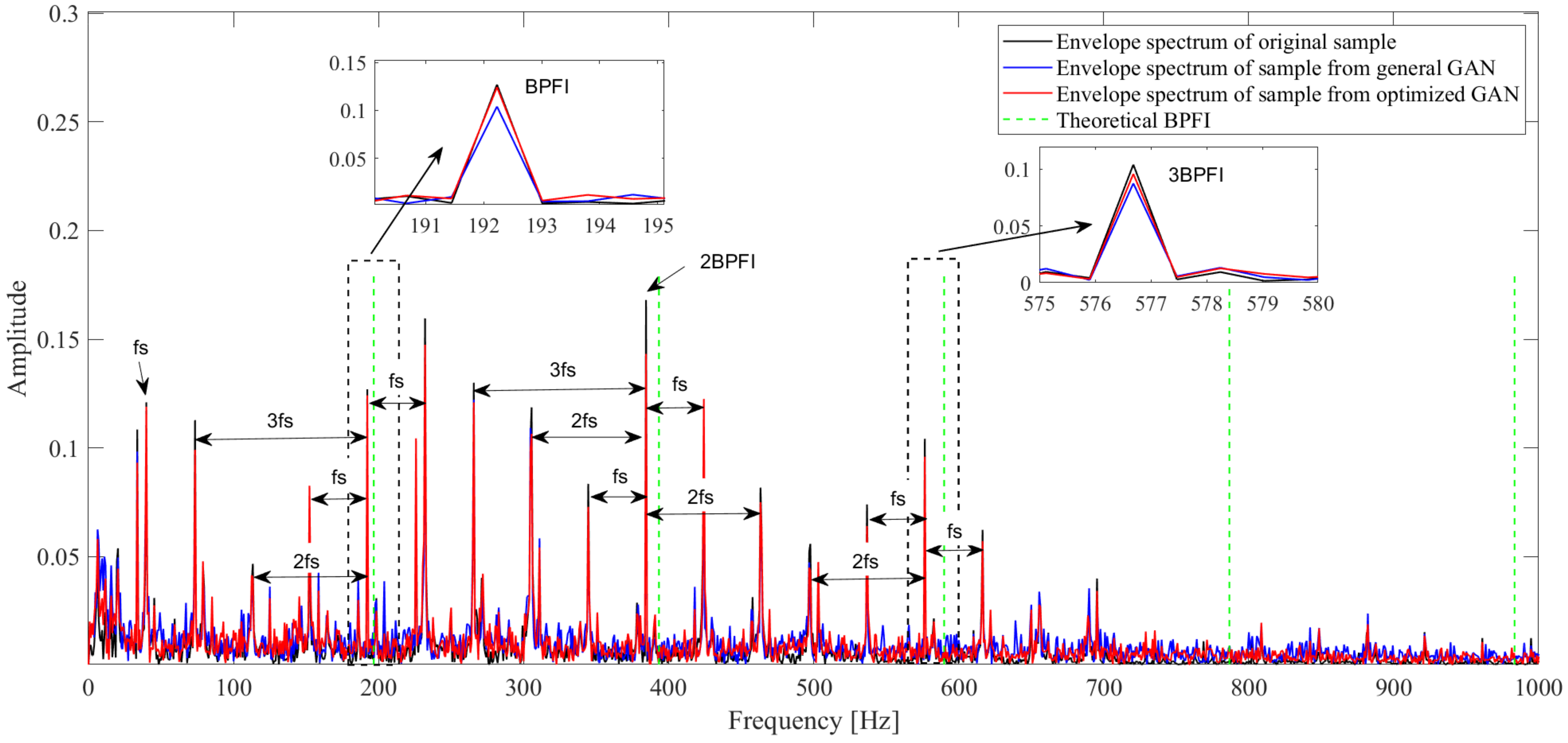
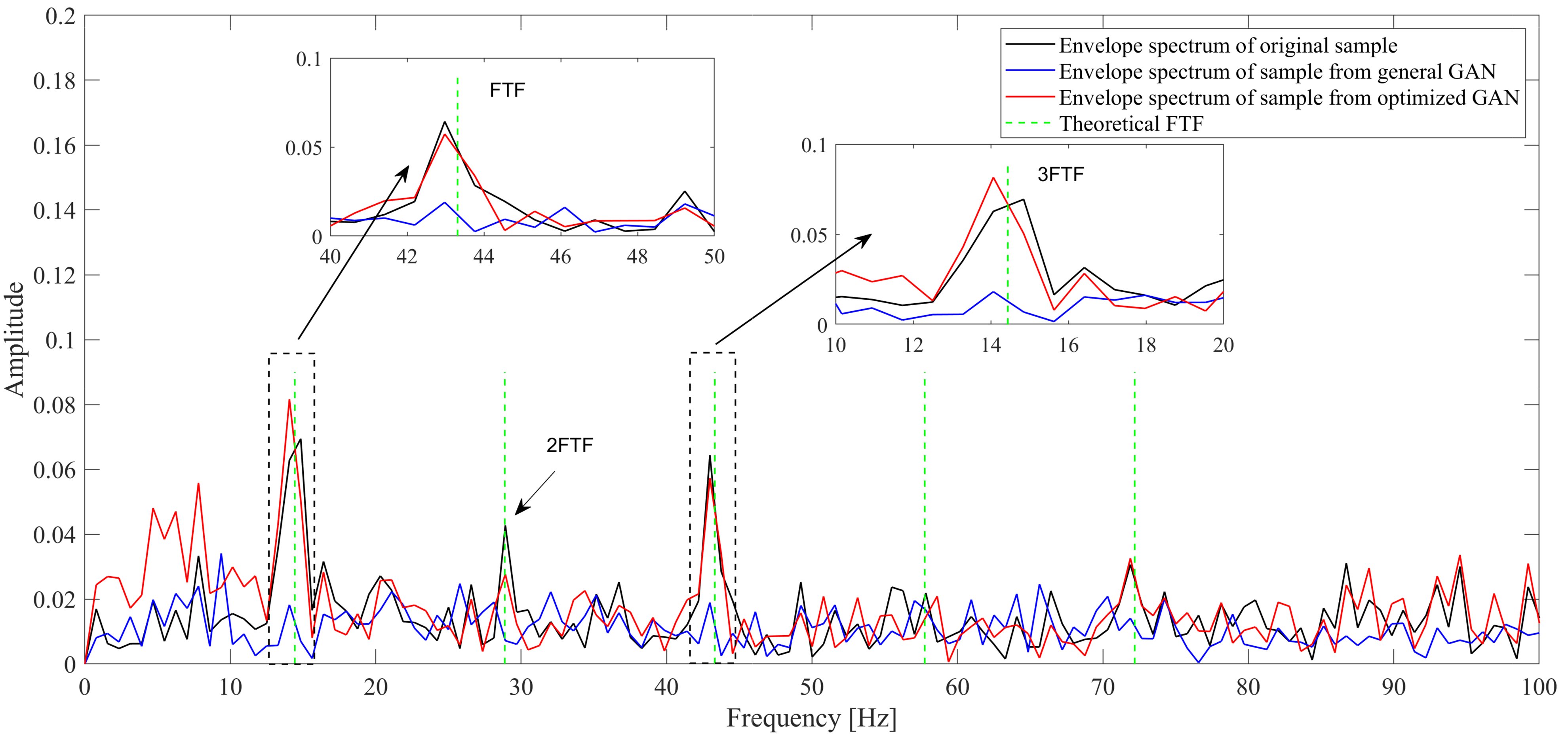
Apart from the overall similarity in time domain, the signal characteristics in the frequency domain are the same or even more important for the fault diagnosis. In this study, the envelope spectrum is processed on the original and generated samples. As only the 1st to 5th F C F s are considered in this study, the signal is first filtered by a low-pass filter of 1000 Hz, and then the envelope spectrum is extracted by Hilbert transform and Fast Fourier Transform. The results are displayed in Figure 7, Figure 8 and Figure 9. Take Figure 7 as an example, which gives the envelope spectrum of bearing 2_1, where the black line is the result of the original measurement, the blue line stands for the sample generated by the general GAN, and the red line symbolizes the sample from the optimized GAN. The theoretical B P F I is also provided by the green dash line. We can find that the envelope spectrum of samples generated by the optimized GAN is similar to the original one, while it appears clearly different from that of the samples generated by the general GAN, especially the amplitudes at the real fault characteristic frequencies. Two locally enlarged views in Figure 7 show that the amplitude from the sample generated by the optimized GAN is much closer to that of the original sample, compared with the sample from the general GAN. The phenomenon is the same for the inner race fault (bearing 3_3), as well as the cage fault (bearing 2_3), which confirms that the optimized GAN can efficiently promote the generated signals to capture more accurate fault characteristics in the frequency domain. As for the other peaks besides fault characteristic ones, especially for the inner race fault, we can find that most of them are caused by the modulation from the shaft frequency and its harmonics, which is consistent with the previous research [24]. Additionally, the deviation between the actual F C F s and the corresponding theoretical values can be explained by many factors, such as the frequency resolution of 0.7814 Hz, the occurrence of rolling element sliding, and the transient contact angles under high external load.
Table 7, Table 8 and Table 9 summarize the sample frequencies and amplitudes at the corresponding F C F and harmonics, as well as the relative error percentage of these two features between the generated and original samples. The comparison in Table 7 shows that, for all the 1st–5th order B P F I s, the frequencies and amplitudes of samples generated by the optimized GAN are much closer to the original ones than those of samples produced by the general GAN. For the sample generated by the optimized GAN, the frequency error percentage under all five orders of B P F I is zero, while the sample generated by the general GAN cannot fully capture the actual B P F I in the original ones, even though the deviation error is 0.34% and only exists in the 5th order B P F I . However, if we focus on the amplitudes under B P F I , the optimized GAN shows much more superiority over the general one. The amplitude errors under all 5 orders of B P F I from the samples generated by the optimized GAN are much smaller than those from the general GAN. Take the 2nd B P F I as an example; the actual amplitude from the original samples is 0.062, while the corresponding amplitudes of the samples from the general GAN and the optimized GAN are 0.023 and 0.047, respectively. The relative error percentage of amplitude drops from 62.0% to 23.8%. The above analysis confirms that the modification term L f r e q u e n c y in the GAN’s generator loss function can enable the GAN to capture the fault information in the frequency domain. The same conclusion can be also drawn based on the results in Table 8 and Table 9.
In summary, data generation results show that both the general GAN and the optimized GAN can generate similar samples compared to the original ones. However, the samples generated by the optimized GAN have higher similarity to the original one than that generated by the general GAN, especially at the F C F and harmonics in the frequency domain. More specifically, data generation for one fault type under different working conditions, such as bearing 2_1 and bearing 3_3, proves that the optimized GAN method can be applied to the bearings under the different working conditions. Furthermore, the results of bearing 2_1 (inner race fault) and bearing 2_3 (cage fault) demonstrate that the optimized GAN method adapts to the bearings with different defect types.

4.2. Fault Diagnosis Based on CNN_GAN

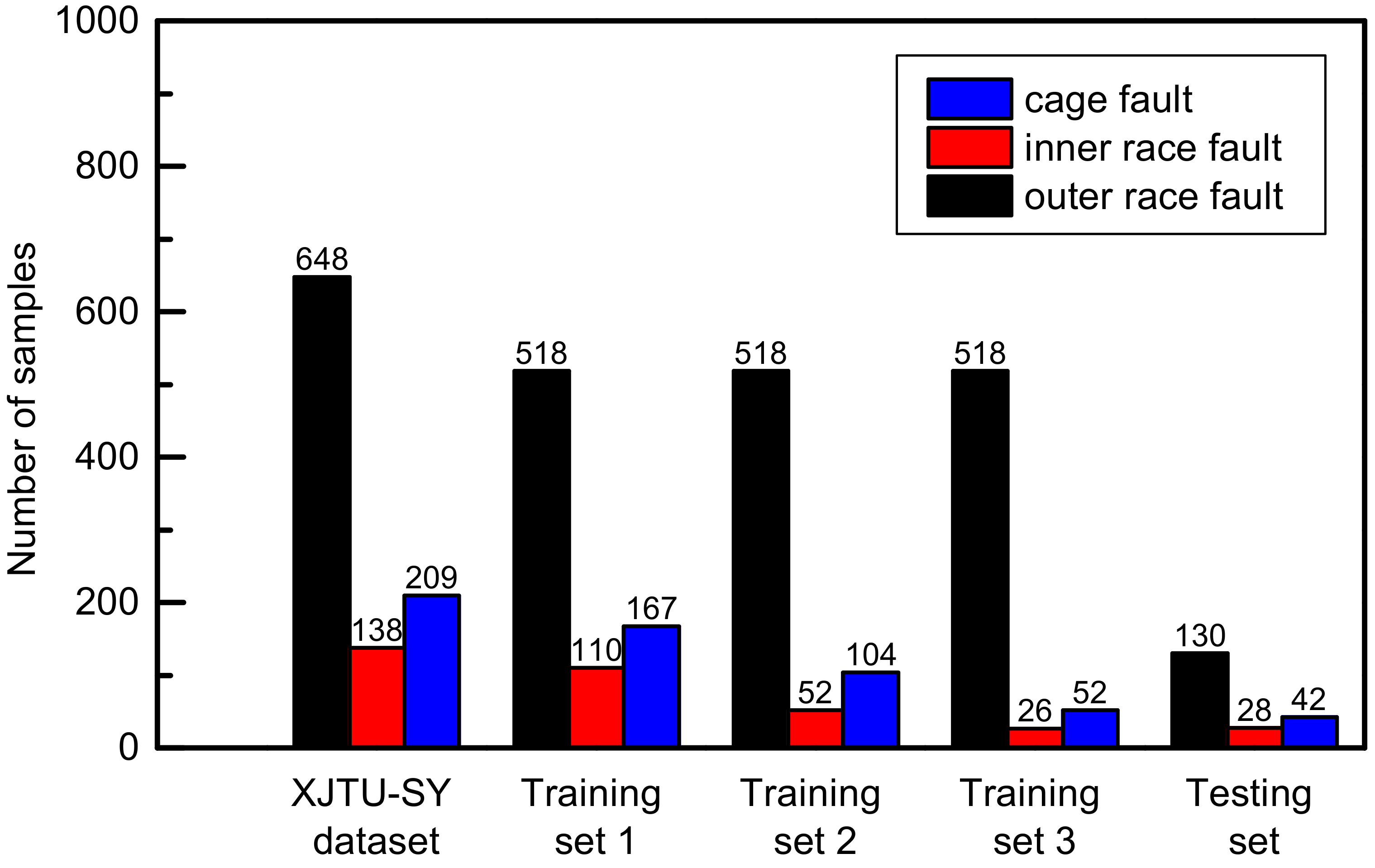
As introduced in Section 3, there are 648 outer race fault samples, 138 inner race fault samples, and 209 cage fault samples. In other words, the imbalance ratio of XJTU-SY bearing datasets is nearly 5:1:1.5 (outer race fault samples: inner race fault samples: cage fault samples). Besides, 80% of these samples are divided into the training set, with the remaining 20% as the test set. To fully evaluate the positive effect that the GAN has on CNN when dealing with the unbalanced datasets, two more training sets with the imbalance ratios of 10:1:2 and 20:1:2 are built by randomly selecting fewer inner race fault and cage fault samples from the XJTU-SY bearing datasets (the training dataset in Table 5), while the test set is fixed the same as the test set in Table 5. The sample composition of three training sets with different imbalance ratios and the test sets is illustrated in Figure 10.
Before validating the test set, on the one hand, CNN is trained on the training sets with the different imbalance ratios, in which the outer race fault has much more samples than the inner race fault and the cage fault. On the other hand, the unbalanced training sets are extended with the optimized GAN by generating more inner race fault and cage fault samples. After data generation, all 3 fault types in the extended training sets have the same sample size, with 518 samples individually. In other words, the ratios between the outer race fault samples, the inner race fault samples, and the cage fault samples become balanced. The general CNN and CNN_GAN mentioned above are validated with the same testing set. The difference between these two CNNs is that the former is trained with the imbalanced training set and then directly validated with the testing set, while the latter is trained with the extended dataset that has been balanced with the collaboration of the GAN and CNN and then validated with the testing set. The CNNs’ performance comparison on the testing set is displayed in Table 10.
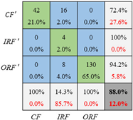
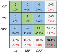
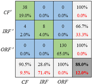
For the general CNN, the fault diagnosis accuracy decreases from 98% to 88% when the imbalance ratio of training set increases from 5:1:1.5 to 10:1:2, and it sharply drops to 68% when the imbalance ratio further raises to 20:1:2. This confirms that the imbalance ratio of training datasets has a great influence on the CNN’s performance. On the contrary, if a CNN is trained on the extended datasets that have been augmented with the generated samples from the optimized GAN, the CNN’s performance can be significantly improved. For instance, when CNN_GAN is trained with the training sets 1 and 2 that have been extended and balanced, its fault classification accuracy on the testing sets achieves up to 100% and 90%, respectively. Even when the imbalance ratio raises up to 20:1:2, the CNN_GAN’s fault classification accuracy still maintains 88%. Under all 3 training sets, the CNN_GAN has a smaller average cross-entropy error compared with the general CNN, which proves that the GAN can efficiently improve the CNN’s fault diagnosis performance by generating new samples when dealing with the unbalanced datasets. Additionally, Table 10 shows that a training set with a higher imbalance ratio brings lower CNN classification accuracy, even after being balanced by data generation with a GAN. Though CNN_GAN performs better than CNN, the change tendencies of both two networks over increasing imbalance ratios are consistent, which indicates there exists an imbalance ratio limitation of the training set that CNN_GAN can handle with, especially for a predefined CNN’s performance index. For example, in this case, if the target of the CNN’s classification accuracy on the fixed imbalanced dataset is set as 90%, then, the CNN_GAN can deal with the training set with a maximum imbalance ratio of 10:1:2.
Besides the accuracy and cross-entropy, the confusion matrix gives more details of the classification for each label. As presented in Table 11, all these 3 cases are validated on the same dataset as the testing set in Figure 10 but trained with one of the three training sets with different imbalance ratios in Figure 10. Specifically, the general CNN is trained with the original unbalanced datasets, and the CNN_GAN is trained with the extended datasets that have been balanced by the optimized GAN. In these confusion matrices, the misclassified samples mainly come from the inner race fault and the cage fault because the outer race fault samples are dominant in each training set. Moreover, the higher the imbalance ratio is, the higher the prediction error is. With further comparison between the CNN and CNN_GAN, it can be found that the CNN_GAN achieves higher overall accuracy than the general CNN. In addition, the fault classification accuracy of both the inner race fault and the cage fault can be improved if the optimized GAN is employed to generate the inner race and cage fault samples. For example, under set 1 and set 2, the CNN’s classification accuracy on the inner race fault increases from 85.7% to 100% and from 14.3% to 28.6%, respectively. With respect to the cage fault, the CNN’s diagnosis accuracy increases remarkably from 4.8% to 90.5% under set 3. The result can be explained as: in the unbalanced dataset, the dominant fault type samples have much more influence on the loss function, which, therefore, push the CNN forward to extract more local features that are only shared by the dominant fault type, with CNN’s ability lost to extract more general and robust features that can distinguish different fault types. This means that CNN has dropped into overfitting. While, for the CNN_GAN, the imbalanced data has been balanced, which means there are no dominant fault types in the training set. Therefore, the trained CNN_GAN can avoid overfitting and have the capability to capture fault features that can be used to recognize the fault types and be simultaneously robust enough. Based on the above analysis, it can be concluded that the balanced training dataset can effectively enhance the CNN’s fault classification performance, and the optimized GAN can efficiently transform the unbalanced dataset into the balanced one by generating samples for the fault types that have limited data.

5. Conclusions

To solve the CNN’s performance reduction problem under the unbalanced datasets, an improved GAN is proposed to generate new data for the fault class with limited samples. The work can be summarized as follows:
  • A collaborative network GAN_CNN is developed. The GAN generates an almost balanced dataset with data augmentation for the inner ring and the cage fault samples. Once the generated samples are added, the CNN evaluates the extended dataset quality and outputs the fault classification result to modify the loss function of the GAN’s generator.
  • Besides the overall similarity, the similarity on the envelope spectrum is considered when building the GAN. The envelope spectrum error from the 1st-5th order F C F between the experimental data and the generated data is taken as a correction term to the general cross-entropy based loss function of the GAN’s generator.
Experimental validation is carried on the XJTU-SY bearing dataset. Results confirm the effectiveness of an optimized GAN and the collaborative structure of the CNN_GAN. The following are the main conclusions:
  • When constructing the loss function for a GAN, the GAN performance can be improved by considering the envelope spectrum error. The generated samples have higher fidelity and contain more accurate fault information, which, in turn, contribute to the CNN’s accuracy improvement.
  • The collaborative network CNN_GAN performs better than the GAN or the CNN. The GAN generates more accurate data if the CNN’s classification results are considered into the GAN’s loss function. The CNN’s fault classification accuracy can be significantly enhanced after the GAN generates more data for the unbalanced training dataset.
Though only the idea is validated with CNN_GAN in this paper, it can be extended with other methods. For example, the fault characteristic spectrum can be replaced by other metrics characterizing bearing fault status. With regard to the outlook, we will focus on the extension of this method and try to develop a physics-guided GAN. Validation with more experimental data and application cases will also be addressed in the future.

Author Contributions

Conceptualization, D.R. and C.G.; methodology, D.R.; software, X.S. and D.R.; validation, X.S.; formal analysis, D.R. and X.S.; investigation, D.R.; resources, D.R.; data curation, X.S.; writing—original draft preparation, X.S. and D.R.; writing—review and editing, C.G. and J.Y.; visualization, D.R. and J.Y.; supervision, C.G.; project administration, C.G.; funding acquisition, D.R. All authors have read and agreed to the published version of the manuscript.

Funding

This research was funded by CSC (China Scholarship Council) scholarship (201806250024) and Zhejiang Lab’s International Talent Fund for Young Professionals.

Institutional Review Board Statement

Not applicable.

Informed Consent Statement

Not applicable.

Data Availability Statement

The original experimental data can be downloaded from: http://biaowang.tech/xjtu-sy-bearing-datasets, and the data samples generated by optimized GAN for this study can be found in the following web-based repository: https://www.dropbox.com/sh/aqtzfb514x8hymd/AAB-8cayG5dDsn0z_FFuiNosa?dl=0.

Acknowledgments

Acknowledgment is made for the XJTU-SY bearing dataset published by Xi’an Jiaotong University.

Conflicts of Interest

The authors declare no conflict of interest.

Abbreviations

The following abbreviations are used in this manuscript:
CNNConvolutional Neural Networks
GANGenerative Adversarial Networks
FCFFault characteristic frequency
LSTMLong Short Term Memory
BPFOBall Passing Frequency on Outer race
BPFIBall Passing Frequency on Inner race
FTFFundamental Train Frequency

References

  1. Li, N.; Lei, Y.; Lin, J.; Ding, S.X. An improved exponential model for predicting remaining useful life of rolling element bearings. IEEE Trans. Ind. Electron. 2015, 62, 7762–7773. [Google Scholar] [CrossRef]
  2. Janssens, O.; Slavkovikj, V.; Vervisch, B.; Stockman, K.; Loccufier, M.; Verstockt, S.; Van de Walle, R.; Van Hoecke, S. Convolutional neural network based fault detection for rotating machinery. J. Sound Vib. 2016, 377, 331–345. [Google Scholar] [CrossRef]
  3. Eren, L.; Ince, T.; Kiranyaz, S. A generic intelligent bearing fault diagnosis system using compact adaptive 1D CNN classifier. J. Signal Process. Syst. 2019, 91, 179–189. [Google Scholar] [CrossRef]
  4. Zhang, W.; Peng, G.; Li, C. Bearings fault diagnosis based on convolutional neural networks with 2-D representation of vibration signals as input. MATEC Web Conf. 2017, 95, 13001. [Google Scholar] [CrossRef] [Green Version]
  5. Guo, X.; Chen, L.; Shen, C. Hierarchical adaptive deep convolution neural network and its application to bearing fault diagnosis. Measurement 2016, 93, 490–502. [Google Scholar] [CrossRef]
  6. Wang, D.; Guo, Q.; Song, Y.; Gao, S.; Li, Y. Application of multiscale learning neural network based on CNN in bearing fault diagnosis. J. Signal Process. Syst. 2019, 91, 1205–1217. [Google Scholar] [CrossRef]
  7. Sabir, R.; Rosato, D.; Hartmann, S.; Guehmann, C. Lstm based bearing fault diagnosis of electrical machines using motor current signal. In Proceedings of the 18th IEEE International Conference On Machine Learning And Applications (ICMLA), Boca Raton, FL, USA, 16–19 December 2019; pp. 613–618. [Google Scholar]
  8. Yu, L.; Qu, J.; Gao, F.; Tian, Y. A novel hierarchical algorithm for bearing fault diagnosis based on stacked LSTM. Shock Vib. 2019. [Google Scholar] [CrossRef] [PubMed]
  9. Qiu, D.; Liu, Z.; Zhou, Y.; Shi, J. Modified Bi-Directional LSTM Neural Networks for Rolling Bearing Fault Diagnosis. In Proceedings of the ICC 2019-IEEE International Conference on Communications (ICC), Shanghai, China, 20–24 May 2019; pp. 1–6. [Google Scholar]
  10. Pan, H.; He, X.; Tang, S.; Meng, F. An improved bearing fault diagnosis method using one-dimensional CNN and LSTM. J. Mech. Eng 2018, 64, 443–452. [Google Scholar]
  11. Xiao, D.; Huang, Y.; Qin, C.; Liu, Z.; Li, Y.; Liu, C. Transfer learning with convolutional neural networks for small sample size problem in machinery fault diagnosis. Proc. Inst. Mech. Eng. Part C J. Mech. Eng. Sci. 2019, 233, 5131–5143. [Google Scholar] [CrossRef]
  12. Zhou, F.; Yang, S.; Fujita, H.; Chen, D.; Wen, C. Deep learning fault diagnosis method based on global optimization GAN for unbalanced data. Knowl.-Based Syst. 2020, 187, 104837. [Google Scholar] [CrossRef]
  13. Cordón, I.; García, S.; Fernández, A.; Herrera, F. Imbalance: Oversampling algorithms for imbalanced classification in R. Knowl.-Based Syst. 2018, 161, 329–341. [Google Scholar] [CrossRef]
  14. Ren, S.; Zhu, W.; Liao, B.; Li, Z.; Wang, P.; Li, K.; Chen, M.; Li, Z. Selection-based resampling ensemble algorithm for nonstationary imbalanced stream data learning. Knowl.-Based Syst. 2019, 163, 705–722. [Google Scholar] [CrossRef]
  15. Shao, S.; Wang, P.; Yan, R. Generative adversarial networks for data augmentation in machine fault diagnosis. Comput. Ind. 2019, 106, 85–93. [Google Scholar] [CrossRef]
  16. Zhang, W.; Li, X.; Jia, X.D.; Ma, H.; Luo, Z.; Li, X. Machinery fault diagnosis with imbalanced data using deep generative adversarial networks. Measurement 2020, 152, 107377. [Google Scholar] [CrossRef]
  17. Yuan, B. Efficient hardware architecture of softmax layer in deep neural network. In Proceedings of the 29th IEEE International System-on-Chip Conference (SOCC), Seattle, WA, USA, 6–9 September 2016; pp. 323–326. [Google Scholar]
  18. Kramer, O. Scikit-learn. In Machine Learning for Evolution Strategies; Springer: Berlin/Heidelberg, Germany, 2016; pp. 45–53. [Google Scholar]
  19. Wang, B.; Lei, Y.; Li, N.; Li, N. A hybrid prognostics approach for estimating remaining useful life of rolling element bearings. IEEE Trans. Reliab. 2018, 69, 401–412. [Google Scholar] [CrossRef]
  20. Randall, R.B.; Antoni, J. Rolling element bearing diagnostics—A tutorial. Mech. Syst. Signal Process. 2011, 25, 485–520. [Google Scholar] [CrossRef]
  21. Niu, L.; Cao, H.; He, Z.; Li, Y. A systematic study of ball passing frequencies based on dynamic modeling of rolling ball bearings with localized surface defects. J. Sound Vib. 2015, 357, 207–232. [Google Scholar] [CrossRef]
  22. Saruhan, H.; Saridemir, S.; Qicek, A.; Uygur, I. Vibration analysis of rolling element bearings defects. J. Appl. Res. Technol. 2014, 12, 384–395. [Google Scholar] [CrossRef]
  23. Devogele, T.; Etienne, L.; Esnault, M.; Lardy, F. Optimized discrete fréchet distance between trajectories. In Proceedings of the 6th ACM SIGSPATIAL Workshop on Analytics for Big Geospatial Data, Redondo Beach, CA, USA, 7–10 November 2017; pp. 11–19. [Google Scholar]
  24. Mishra, C.; Samantaray, A.; Chakraborty, G. Ball bearing defect models: A study of simulated and experimental fault signatures. J. Sound Vib. 2017, 400, 86–112. [Google Scholar] [CrossRef]
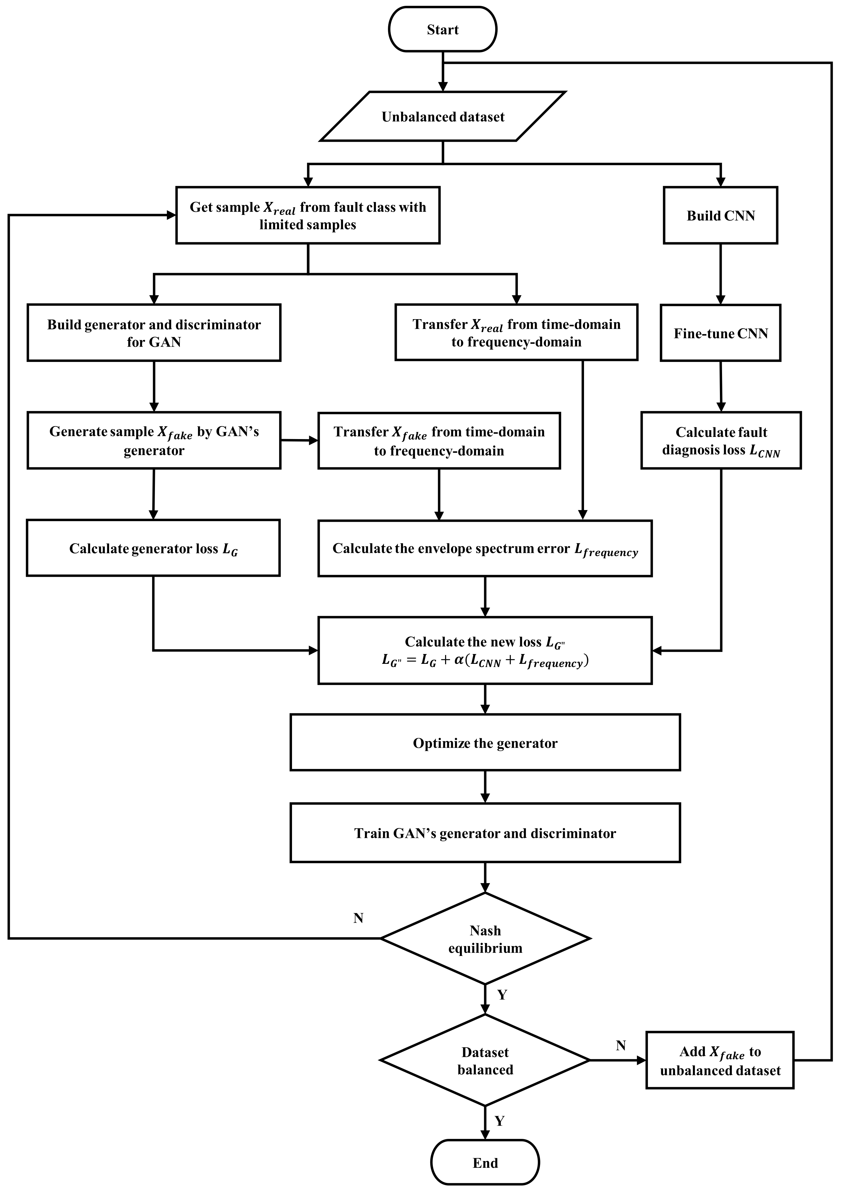
Figure 1. Collaborative training structure of the GAN and CNN.
Lubricants 09 00105 g001
Figure 2. Architecture of generator and discriminator in the GAN.
Lubricants 09 00105 g002
Figure 3. XJTU-SY experimental setup [19].
Lubricants 09 00105 g003
Figure 4. Complete life cycle of bearing 1_1.
Lubricants 09 00105 g004
Figure 5. Illustration of data reshape.
Lubricants 09 00105 g005
Figure 6. Comparison between original sample and generated sample in time domain; (a), (b) and (c) represent bearing 2_1, bearing 2_3 and bearing 3_3 respectively, while (1), (2) and (3) represent the original sample, general GAN and optimized GAN respectively.
Lubricants 09 00105 g006
Figure 7. Envelope spectrum comparison: inner race fault of bearing 2_1.
Lubricants 09 00105 g007
Figure 8. Envelope spectrum comparison: inner race fault of bearing 3_3.
Lubricants 09 00105 g008
Figure 9. Envelope spectrum comparison: cage fault of bearing 2_3.
Lubricants 09 00105 g009
Figure 10. Composition of training sets and the test set.
Lubricants 09 00105 g010
Table 1. Hyperparameters of the GAN.
HyperparametersValues
Initial learning rate of generator0.0001
Initial learning rate of discriminator0.0001
Kernel size of discriminator’s 1st layer 8 × 8
Kernel size of discriminator’s other layers 4 × 4
Number of filters in discriminator’s n-th layer 16 × 2 n 1
Kernel size of generator’s last layer 8 × 8
Kernel size of discriminator’s other layers 4 × 4
Number of filters in generator’s n-th layer 512 / 2 n 1
Max epochs2000
Table 2. Hyperparameters of the CNN.
HyperparametersValues
Initial learning rate0.0002
Max epochs1000
Batch size20
Kernel size of 1st layer 7 × 7
Kernel size of other layers 3 × 3
Number of filters in n-th layer 16 × 2 n 1
Table 3. Specifications of bearing parameters.
ParametersValuesParametersValues
Inner raceway diameter 29.30   m m Ball diameter 7.92   m m
Outer raceway diameter 39.80   m m Number of balls8
Pitch diameter 34.55   m m Initial contact angle0
Table 4. Data specification of XJTU-SY bearing dataset.
ConditionTest BearingMeasurement Sample SizeFault Location
(1)
f s = 35 Hz
F r = 12 k N
bearing 1_1123outer ring
bearing 1_2161outer ring
bearing 1_3158outer ring
bearing 1_4122cage
bearing 1_552outer ring & inner ring
(2)
f s = 37.5   Hz
F r = 11 k N
bearing 2_1491inner ring
bearing 2_2161outer ring
bearing 2_3533cage
bearing 2_442outer ring
bearing 2_5339outer ring
(3)
f s = 40 Hz
F r = 10 k N
bearing 3_12538outer ring
bearing 3_22496inner ring & element & cage & outer ring
bearing 3_3371inner ring
bearing 3_41515inner ring
bearing 3_5114outer ring
Table 5. Sample size of different fault types.
Fault LocationTest BearingMeasurement Sample SizeTraining SetsTest Sets
Outer racebearing 1_158518130
bearing 1_2108
bearing 1_369
bearing 2_277
bearing 2_412
bearing 2_5173
bearing 3_155
bearing 3_5106
Inner racebearing 2_12611028
bearing 3_328
bearing 3_484
Cagebearing 1_4116742
bearing 2_3208
Table 6. Cosine similarity of samples in time domain.
Generated SampleCosine Similarity
GANOptimized GAN
bearing 2_10.32140.3739
bearing 3_30.33740.3408
bearing 2_30.20090.2675
Table 7. Amplitudes and frequencies of bearing 2_1 at 1st–5th B P F I .
Sample SourceParameter1st— BPFI 2nd— BPFI 3rd— BPFI 4th— BPFI 5th— BPFI
Original sampleFrequency (Hz)178.944357.889536.833715.788931.449
Amplitude0.1760.0620.1240.0720.020
Sample from general GANFrequency (Hz)178.944357.889536.833715.788928.323
Error (%)00000.34
Amplitude0.1170.0230.0860.0530.011
Error (%)33.362.030.126.144.1
Sample from optimized GANFrequency178.944357.889536.833715.788931.449
Error (%)00000
Amplitude0.1490.0470.1060.0600.018
Error (%)15.323.814.216.59.4
Table 8. Amplitudes and frequencies of bearing 3_3 at 1st–5th B P F I .
Sample SourceParameter1st— BPFI 2nd— BPFI 3rd— BPFI 4th— BPFI 5th— BPFI
Original sampleFrequency (Hz)192.229384.457576.686808.767994.744
Amplitude0.1270.1680.1040.0150.013
Sample from general GANFrequency (Hz)192.229384.457576.686808.767990.055
Error (%)00000.5
Amplitude0.1040.1310.0880.0190.006
Error (%)18.022.115.926.049.5
Sample from optimized GANFrequency (Hz)192.229384.457576.686808.767961.143
Error (%)00000
Amplitude0.1240.1430.0960.0200.011
Error (%)2.214.77.926.714.4
Table 9. Amplitudes and frequencies of bearing 2_3 at 1st–5th F T F .
Sample SourceParameter1st— FTF 2nd— FTF 3rd— FTF 4th— FTF 5th— FTF
Original sampleFrequency (Hz)14.84728.91242.97857.82571.890
Amplitude0.0690.0430.0640.0220.031
Sample from general GANFrequency14.06628.13142.97857.04371.890
Error (%)5.32.701.40
Amplitude0.0180.0190.0190.0200.014
Error73.355.470.610.754.1
Sample from optimized GANFrequency (Hz)14.06628.91242.97858.60671.890
Error (%)5.3001.40
Amplitude0.0820.0280.0570.0210.033
Error (%)17.535.310.94.66.4
Table 10. Comparison of fault diagnosis performance between CNN and CNN_GAN.
Imbalance RatioCNNCNN_GAN
AccuracyCross-Entropy ErrorAccuracyCross-Entropy Error
Training set 1 (5:1:1.5)98%0.6071100%0.5645
Training set 2 (10:1:2)88%0.701390%0.6642
Training set 3 (20:1:2)68%0.847888%0.7012
Table 11. Fault diagnosis confusion matrix under three training sets.
Diagnosis NetworkConfusion Matrix on Testing Set
Training with Set 1
Unbalance Ratio (5:1:1.5)
Training with Set 2
Unbalance Ratio (10:1:2)
Training with Set 3
Unbalance Ratio (20:1:2)
CNN Lubricants 09 00105 i001 Lubricants 09 00105 i002 Lubricants 09 00105 i003
CNN_GAN Lubricants 09 00105 i004 Lubricants 09 00105 i005 Lubricants 09 00105 i006
Target label: CF-cage fault, IRF-inner race fault, ORF-outer race fault; prediction label: CF’-cage fault, IRF’-inner race fault, ORF’-outer race fault.
Publisher’s Note: MDPI stays neutral with regard to jurisdictional claims in published maps and institutional affiliations.