Nonlinear Dynamic Response of an Unbalanced Flexible Rotor Supported by Elastic Bearings Lubricated with Piezo-Viscous Polar Fluids

Abstract

On the basis of the V. K. Stokes micro-continuum theory, the effects of couple stresses on the nonlinear dynamic response of the unbalanced Jeffcott’s flexible rotor supported by layered hydrodynamic journal bearings is presented in this paper. A nonlinear transient modified Reynolds’ equation is derived and discretized by the finite element method to obtain the fluid-film pressure field as well as the film thickness by means of the implicit Euler method. The nonlinear orbits of the rotor center are determined by solving the nonlinear differential equations of motion with the explicit Euler’s scheme taking into account the flexibility of rotor. According to the obtained results, the combined effects of couple stresses due to the presence of polymer additives in lubricant and the pressure dependent viscosity on the nonlinear dynamic response of the rotor-bearing system are significant and cannot be ignored or overlooked. As expected, these effects are more noticeable for polymers characterized by higher length molecular chains.

1. Introduction

Rotating machines such as turbo-machines are the most important class of machinery that are extensively used in diverse engineering applications such as power stations, aircraft propulsion systems, etc. These machines include at least one rotor generally supported by oil-lubricated journal bearings which must not be considered to be passive elements, but elements which sensitively affect the dynamic behavior and stability of the rotor.

The design trend of such mechanical systems in modern engineering is towards lower weight and operating at super critical speeds.

The role of rotor is to transmit or to transform the mechanical power. It is often of very much complex realization and includes bladed disks or impellers, gears, for example.

The correct prediction of dynamic behavior is extremely essential when the rotor rotating at high speeds is made very flexible. Further, the dynamic behavior of a rotor-bearing system largely depends on the nonlinear dynamic characteristics of oil-lubricated bearings which may be a source of self-induced vibrations popularly known as oil whirl and oil whip phenomena which occur especially when the rotor-bearing system is lightly loaded or operates at low values of eccentricity ratio. This vibratory motion can cause considerable mechanical problems, like rubbing between shaft and bearing, blades and stator in turbo-machines, or more generally vibrations of the whole rotating machinery. In 1924, Newkirk and Taylor [1] first demonstrated that the oil whirl is caused by the dynamic oil film forces in the bearings. Since then, a number of researchers have focused their theoretical and experimental studies on the stability, bifurcation, and chaos of rotor-bearing systems, and a significant progress in rotor-dynamics field has been made [2,3,4,5,6,7,8,9,10,11,12,13,14,15,16,17,18,19,20,21].

Of the many published works, the most extensive portion of the literature on rotor dynamics is concerned with determining critical speeds, natural whirl frequencies, instability thresholds, and imbalance response. In these works generally based on the linearized theory, the authors used in their analysis several assumptions among them the rotor and bearings are assumed to be rigid. Moreover, the linear stability analysis predicts the stability limits only under small disturbances, it does not give any information about the transient phenomena of a rotor-bearing system under large disturbances. Those phenomena should be studied by means of a nonlinear stability theory.

On the other hand, the rheological behavior of mineral oils used as lubricants in industrial machinery is influenced by the presence of additives such as Viscosity Index (VI) improver polymers which are characterized by long-chains. Thus, Oils containing VI additives such as multi-grade engine oils must be considered as non-Newtonian fluids and can be modeled as polar fluids. Experimentally, it was found that the presence of dissolved polymer in the lubricant increases the load carrying capacity of the lubricating film and decreases the friction coefficient [22,23].

In order to better describe the rheological behavior of this kind of non-Newtonian lubricant so-called couple stress fluid, different micro-continuum theories have been developed [24,25]. The Stokes micro-continuum theory [26] is the simplest theory of fluids proposed in the technical literature, which allows the polar effects such as the presence of couple-stresses m_i and body couples noted ℓ_i in addition to the body forces and surface forces Figure 1.

Figure 1. Balance of forces and couples acting on elementary volume according to V. K. Stokes theory.

Figure 1. Balance of forces and couples acting on elementary volume according to V. K. Stokes theory.

The iso-volume couple-stress fluids are characterized by two constants, namely $\mu$ and $\eta$ whereas only one parameter appears for a Newtonian iso-volume fluid which is the dynamic viscosity $\mu$. The new material constant $\eta$ is responsible for couple-stress property. In the literature, the effects of couple-stresses on the behavior of journal bearings are studied by defining the dimensionless couple-stress parameter ${\ell }^{\ast }=\frac{\ell }{C}$ where $\ell =\sqrt{\frac{\eta }{\mu }}$ which has the dimension of length and can be thought of as a fluid property depending on the size of the high polymer molecule.

Owing to its relative mathematical simplicity, the couple-stress fluid model has been widely applied to analyze various hydrodynamic lubrication problems: hydrostatic thrust bearings, slider bearings, rolling bearings, squeeze film bearings, layered journal bearings, and dynamically loaded engine journal bearings [27,28,29,30,31,32,33]. The theoretical results obtained showed that the presence of the couple-stress provides an enhancement in the load carrying capacity, improve the dynamic performance characteristics and the stability of journal bearings, and lengthens the response time of the squeeze film action of the system as compared to the Newtonian lubricant case. It was also shown that the effects of couple stress are more pronounced for high values of the couple-stress parameter $\ell$.

According to the Stokes micro-continuum theory of couple stress fluids [26] together with the variation of viscosity with pressure, the combined effects of piezo-viscous dependency and non-Newtonian couple stresses on wide parallel rectangular-plate squeeze-film characteristics have recently been studied by Lin et al. [34]. The viscosity-pressure relationship used by the authors is that of Barus [35] which is largely used in elastohydrodynamic lubrication analysis. They have found that the combined effects of piezo-viscosity and couple stresses cause an increase in the load carrying capacity and the squeeze film time.

As far as we know, very few research works have been devoted to analyze the nonlinear dynamic behavior of flexible rotors mounted in layered journal bearings lubricated with complex non-Newtonian fluids taking into account the combined effects of fluid couple-stresses, pressure-viscosity dependency, and compliance of the bearing structure.

The main objective of the present research is to theoretically investigate the nonlinear dynamic response of a flexible rotor supported by layered bearings using piezo-viscous couple-stress fluids as lubricants. The elastic deformation of the liner due to the fluid film pressure is calculated using a simplified elasticity model known as the “thin liner model”. So, we assume that the radial deformation at the fluid-liner interface is proportional to the hydrodynamic pressure. On the other hand, the Barus law is used in order to take into account the viscosity-pressure dependency at constant temperature:

$$\mu \left(p\right)={\mu }_0{e}^{\alpha p}$$

(1)

where ${\mu }_0$ is the atmospheric dynamic viscosity, and α is the pressure-viscosity coefficient which can be obtained by plotting the natural logarithm of dynamic viscosity $\mu$ versus pressure p. The slope of the graph corresponds to the value of α. The pressure-viscosity coefficient is a function of the molecular structure of the lubricant and its physical characteristics. If α = 0, the viscosity is then constant and the fluid is considered as iso-viscous.

The pressure-viscosity coefficient of the Barus equation has a value between 1.5–2.4 × 10⁻⁸ (m²/N) for paraffinic oils, and a value between 2.5–3.5 × 10⁻⁸ (m²/N) for aromatic oils according to Klamann [36].

There are various formulae available to calculate the pressure-viscosity coefficient. One of the early ones was derived by Wooster [37]:

$$\alpha =\left(0.6+0.965lo{g}_{10}\left({\mu }_0\right)\right)\times {10}^{-8}$$

(2)

where α is the pressure-viscosity coefficient in (Pa⁻¹), and ${\mu }_0$ is the atmospheric dynamic viscosity in (cP) or (mPa·s). There are also other equations for the calculation of the pressure-viscosity coefficient available in the literature. Some of these equations are accurate for certain fluids and inaccurate for others. One of the problems associated with available formulae is that they only allow the accurate calculation of pressure-viscosity coefficients at low shear rates. An accurate value of this coefficient can be determined experimentally.

The piezo-viscosity effect varies between oils; and it is more considerable for naphthenic oils than paraffinic oils. Water; by contrast shows only a small rise; almost negligible; in viscosity with pressure.

Note that the value of the pressure-viscosity coefficient is in general reduced at higher temperatures, with naphthenic oils being the most severely affected. In some cases even at moderate temperatures, there is a substantial reduction in the pressure-viscosity coefficient.

There are many other formulae for viscosity-pressure relationships. A short review of some of the empirical formulae for the viscosity-pressure relationships is given in [38]. These formulae allow for the calculations of viscosity changes with pressure under various conditions and to various degrees of accuracy.

As a first approximation, we consider the simplest flexible rotor model popularly known as the Jeffcott model (1919). In spite of its age of over 90 years, the Jeffcott rotor is still widely used.

Figure 2 shows a typical Jeffcott rotor. It consists of a simply supported flexible massless shaft with a rigid disc mounted at the mid-span. The disc center of rotation, C, and its center of gravity, G, is offset by a distance, e which is called the unbalance eccentricity. The shaft spin speed is ω and the shaft whirls about the bearing axis with a whirl frequency ν. For present study, synchronous condition has been assumed, i.e., ν = ω. According to the beam theory, the stiffness of the shaft k_r can be expressed as

$$k_r=\frac{\mathrm{load}}{\mathrm{deflection}}=\frac{48E_r{I}_{Gy}}{L_r^3}$$

(3)

where E_r is the Young’s modulus of rotor, $I_{Gy}={\int }_S^{ }{x}^{2}ds=\frac{\pi D^4}{64}$ is the second moment of area of the rotor (shaft) cross-section, and L_r denotes the span of the rotor (shaft).

Figure 2. A typical Jeffcott rotor.

Figure 2. A typical Jeffcott rotor.

The finite element method is used to approach the nonlinear transient pressure equation called in the present study the modified Reynolds’ equation derived from momentum and mass conserving principles for an incompressible and piezo-viscous couple stress fluid using the V. K. Stokes micro-continuum theory [26]. The first order differential equations system resulting from the discretization of the pressure equation is solved by the implicit Euler’s scheme and the relaxed substitution iterative method in order to determine the instantaneous hydrodynamic forces acting on the rotor (shaft), i.e., at each time step. The nonlinear trajectories of the shaft center are obtained by solving the rotor-dynamics equations with a direct integration procedure, namely the explicit Euler’s scheme.

In the parametric study, there are three key parameters dominating the combined effects of the pressure-viscosity dependency, the presence of couple-stresses, and the compliance of the bearing-liner which are the dimensionless viscosity-pressure coefficient $\tilde{\alpha }$, the dimensionless couple stress parameter $\tilde{\ell }$, and the normalized elasticity parameter $\complement$, respectively.

2. Governing Equations

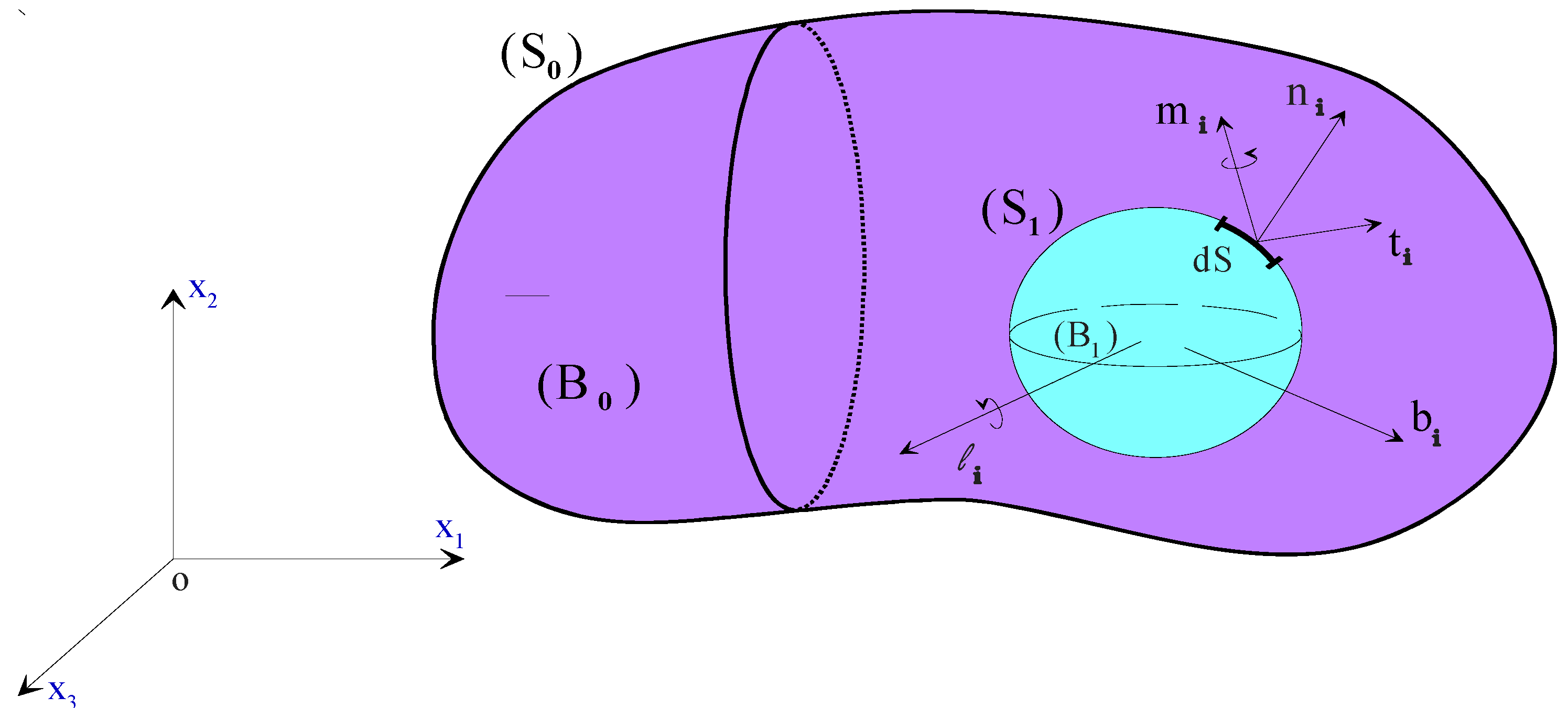
2.1. Momentum Equations of the Polar or Couple Stress Fluid

On the basis of the V. K. Stokes micro-continuum theory (26), when the body forces $b_i$ and body couples ${\ell }_i$ are neglected Figure 1, the motion of the iso-volume polar fluids can be governed by the following equations:

$$\frac{\partial u_i}{\partial x_i}=0$$

(4)

$$\rho \hspace{0.17em}\frac{D{u}_i}{Dt}=\frac{\partial {\sigma }_{ji}}{\partial x_j}$$

(5)

$$M_{ji,j}+e_{ijk}{\sigma }_{jk}=0$$

(6)

where $\frac{D}{Dt}( )=\frac{\partial }{\partial t}( )+u_j\frac{\partial }{\partial x_j}( )$ which is the material time derivative, and ${\sigma }_{ji}\ne {\sigma }_{ij}$.

The constitutive equations for the polar or couple-stresses fluids are given as

$${\sigma }_{ij}=-p{\delta }_{ij}+\mu \left(\frac{\partial u_i}{\partial x_j}+\frac{\partial u_j}{\partial x_i}\right)-\frac{1}{2}{e}_{ijk}{M}_{rk,r}$$

(7)

$$M_{rk}=\frac{1}{3}{M}_{nn}{\delta }_{rk}+4\eta ⥄{\omega }_{k,r}+4{\eta }^{\prime }{\omega }_{r,k}$$

(8)

where ${\mathrm{\omega }}_i=\frac{1}{2}{e}_{irs}\frac{\partial u_s}{\partial x_r}$ is the ith component of the vorticity vector.

If we now consider the case where $\mathrm{\eta }$ and ${\mathrm{\eta }}^{\prime }$ are constants, the conservation of momentum is given by [26]:

$$\rho \frac{D{u}_i}{Dt}=-\frac{\partial p}{\partial x_i}+\frac{\partial }{\partial x_r}\left(\mu \frac{\partial u_i}{\partial x_r}\right)-\eta \hspace{0.17em}\frac{{\partial }^4{u}_i}{\partial x_r\partial x_r\partial x_s\partial x_s}$$

(9)

where $\rho$ is the fluid density, $u_i$ is the velocity component, t is the time, p is the pressure, $\mu$ is the classical shear viscosity and $\eta$ is a new material parameter responsible for the couple-stress property.

Note that the dimension of the material constant $\mathrm{\mu }$ is that of viscosity (ML⁻¹T⁻¹) whereas the dimensions of $\mathrm{\eta }$ is that of momentum (MLT⁻¹). The ratio $\mathrm{\eta }/\mathrm{\mu }$ has dimension of length square and, in the following, we denote this material constant by $\ell$, where $\ell ={\left(\raisebox{1ex}{$\eta $}\!\left/ \!\raisebox{-1ex}{$\mu $}\right.\right)}^{\raisebox{1ex}{$1$}\!\left/ \!\raisebox{-1ex}{$2$}\right.}$. Some experiments for determining the material constants $\mathrm{\mu }$ and $\mathrm{\eta }$ for incompressible fluids are given in Equation (1). Physically, the quantity $\ell$ can be regarded as a characteristic length of the additives which are added to the base oil and which can be polymers or co-polymers.

In thin film theory, the dimension across the film thickness is small compared to the others. From this assumption, we can determine the order of magnitude for the different terms of Equation (9).

The field equations governing the motion of the lubricating oil in the Cartesian coordinates system are:

$$\{\begin{array}{l}\eta \frac{{\partial }^{4}u}{\partial y^4}-\frac{\partial }{\partial y}\left(\mu \frac{\partial u}{\partial y}\right)=-\frac{\partial p}{\partial x}\\ \frac{\partial p}{\partial y}=0\\ \eta \frac{{\partial }^{4}w}{\partial y^4}-\frac{\partial }{\partial y}\left(\mu \frac{\partial w}{\partial y}\right)=-\frac{\partial p}{\partial z}\end{array}$$

(10)

and

$$\overrightarrow{\nabla }\cdot \overrightarrow{V}=\frac{\partial u}{\partial x}+\frac{\partial v}{\partial y}+\frac{\partial w}{\partial z}=0$$

(11)

where $\overrightarrow{V}$ is the flow velocity field.

According to the Barus law, the second term appearing on the left hand side of Equation (10) can be expressed as follows:

$\frac{\partial }{\partial y}\left(\mu \frac{\partial u}{\partial y}\right)={\mu }_0{e}^{\alpha p}\frac{{\partial }^{2}u}{\partial y^2}$ since $\frac{\partial \mu }{\partial y}=\frac{\partial \mu }{\partial p}\frac{\partial p}{\partial y}=0$ according to the second equation of Equation (10).

The boundary conditions at the bearing surfaces (y = 0) and the journal surface (y = h) are:

$$\begin{array}{l}u\left(x,0,z\right)=0\\ w\left(x,0,z\right)=0\end{array}$$

(12)

$$\begin{array}{l}{\frac{{\partial }^{2}u}{\partial y^2}|}_{y=0}=0\\ {\frac{{\partial }^{2}w}{\partial y^2}|}_{y=0}=0\end{array}$$

(13)

$$\begin{array}{l}u\left(x,h,z\right)=U_j\\ w\left(x,h,z\right)=0\end{array}$$

(14)

$$\begin{array}{l}{\frac{{\partial }^{2}u}{\partial y^2}|}_{y=h}=0\\ {\frac{{\partial }^{2}w}{\partial y^2}|}_{y=h}=0\end{array}$$

(15)

Conditions Equations (12) and (14) are the no-slip velocity conditions and conditions Equations (13), (15) result from the fact that the couple-stresses ($-2\eta \frac{{\partial }^{2}u}{\partial y^2}$) and ($-2\eta \frac{{\partial }^{2}w}{\partial y^2}$) vanish at the solid boundary. Using the above boundary conditions, the fluid velocity components u and w for an iso-volume piezo-viscous couple stress fluid are:

$$\begin{array}{l}u\left(x,y,z\right)=U_j\frac{y}{h}+\frac{e^{-2\alpha p}}{2{\mu }_0}\frac{\partial p}{\partial x}\left\{\frac{y\left(y-h\right)}{e^{-\alpha p}}+2{\ell }^2\left[1-\frac{Cosh\left(\frac{2y-h}{2\ell e^{-\frac{1}{2}\alpha p}}\right)}{Cosh\left(\frac{h}{2\ell e^{-\frac{1}{2}\alpha p}}\right)}\right]\right\}\\ w\left(x,y,z\right)=\frac{e^{-2\alpha p}}{2{\mu }_0}\frac{\partial p}{\partial z}\left\{\frac{y\left(y-h\right)}{e^{-\alpha p}}+2{\ell }^2\left[1-\frac{Cosh\left(\frac{2y-h}{2\ell e^{-\frac{1}{2}\alpha p}}\right)}{Cosh\left(\frac{h}{2\ell e^{-\frac{1}{2}\alpha p}}\right)}\right]\right\}\end{array}$$

(16)

h being the fluid film thickness depending on x, z and t variables.

2.2. Modified Transient Nonlinear Piezo-Viscous Reynolds’ Equation and Boundary Conditions

Substituting the expressions of the velocity components u and w from Equation (16) in the continuity Equation (11) and integrating across the film thickness, i.e., with respect to y variable, using the boundary conditions for v given below:

$$\begin{array}{l}v\left(x,0,z\right)=0\\ v\left(x,h,z\right)=V_j=\frac{dh\left(x,z,t\right)}{dt}=\frac{\partial h}{\partial t}+U_j\frac{\partial h}{\partial x}+W_j\frac{\partial h}{\partial z}\end{array}$$

(17)

yields to the following transient nonlinear modified Reynolds’ equation:

$$\overrightarrow{\nabla }\cdot \overrightarrow{Q}=\frac{\partial Q_x}{\partial x}+\frac{\partial Q_z}{\partial z}= -\frac{\partial h}{\partial t}$$

(18)

where

$Q_x=-\frac{G\left(h,\ell ,\alpha ,p\right)}{12{\mu }_0}\frac{\partial p}{\partial x}+\frac{h}{2}{U}_j$, $Q_z=-\frac{G\left(h,\ell ,\alpha ,p\right)}{12{\mu }_0}\frac{\partial p}{\partial z}$, and

$$G\left(h,\ell ,\alpha ,p\right)=h^3{e}^{-\alpha p}-12{\ell }^2\left[h{e}^{-2\alpha p}-2\ell e^{-\frac{5}{2}\alpha p}\tanh \left(\frac{h{e}^{\frac{1}{2}\alpha p}}{2\ell }\right)\right]$$

(19)

$Q_x={\displaystyle \underset{0}{\overset{h}{\int }}u\left(x,y,z\right)dy}$ and $Q_z={\displaystyle \underset{0}{\overset{h}{\int }}w\left(x,y,z\right)dy}$ being the volume flow rate components per unit length in x and z directions, respectively.

According to Equations (17) and (19), Equation (18) becomes

$$\frac{\partial }{\partial x}\left(G\left(h,\ell ,\alpha ,p\right)\frac{\partial p}{\partial x}\right)+\frac{\partial }{\partial z}\left(G\left(h,\ell ,\alpha ,p\right)\frac{\partial p}{\partial z}\right)= 6{\mu }_0\left[U_j\frac{\partial h}{\partial x} +2\frac{\partial h}{\partial t}\right]$$

(20a)

where U_j = ɷR is the linear velocity of the journal surface.

Equation (20a) is known as the modified Reynolds’ equation which is a nonlinear partial differential equation.

For an iso-viscous and nonpolar (Newtonian) fluid for which $\alpha =\eta =0$, Equation (20a) reduces to the standard linear Reynolds’ equation since $G\left(h,\ell ,\alpha ,p\right)=h^3$, i.e.,

$$\frac{\partial }{\partial x}\left(h^3\frac{\partial p}{\partial x}\right)+\frac{\partial }{\partial z}\left(h^3\frac{\partial p}{\partial z}\right)= 6{\mu }_0\left[U_j\frac{\partial h}{\partial x} +2\frac{\partial h}{\partial t}\right]$$

(20b)

Using the non-dimensional quantities (indicated with a superscript asterisk (*))

$\theta =\raisebox{1ex}{$x$}\!\left/ \!\raisebox{-1ex}{$R$}\right.,z^{\ast }=\frac{z}{L},p^{\ast }=\frac{p}{{\mu }_0\omega {\left(\raisebox{1ex}{$R$}\!\left/ \!\raisebox{-1ex}{$C$}\right.\right)}^2},h^{\ast }=\frac{h}{C},\lambda ={\left(R/L\right)}^2,{\alpha }^{\ast }={\mu }_0\omega {\left(\raisebox{1ex}{$R$}\!\left/ \!\raisebox{-1ex}{$C$}\right.\right)}^2\alpha ,\hspace{0.17em}{\ell }^{\ast }=\frac{\ell }{C},\hspace{0.17em}\mathrm{and} t^{\ast }=\omega t$ in Equation (20), the normalized transient modified Reynolds equation for a journal bearing system Figure 3 is obtained in the form

$$\frac{\partial }{\partial \theta }\left(G^{*}\left(h^{*},{\ell }^{*}, {\alpha }^{*},p^{*}\right)\frac{\partial p^{*}}{\partial \theta }\right)+\lambda \frac{\partial }{\partial z^{*}}\left(G^{*}\left(h^{*},{\ell }^{*}, {\alpha }^{*},p^{*}\right)\frac{\partial p^{*}}{\partial z^{*}}\right)=6\frac{\partial h^{*}}{\partial \theta }+12\frac{\partial h^{*}}{\partial t^{*}}$$

(21)

where

$$h^{*}\left(\theta ,z^{*},t^{*}\right)=1+X^{*}\left(t^{*}\right)cos\theta +Y^{*}\left(t^{*}\right)sin\theta +\complement \tilde{p}\left(\theta ,z^{*},t^{*}\right)$$

(22)

In Equation (20), $\left(X^{*},Y^{*}\right)=\left(X,Y\right)/C$ are the Cartesian instantaneous co-ordinates of the journal centre and the parameter $\complement$represents the compliance factor of the elastic bearing-liner which is defined as

$$\complement ={\sigma }_0{t}_h^{*}{C}_d^{*}$$

(23)

where ${\sigma }_0=\frac{\left(1+\sigma \right)\left(1-2\sigma \right)}{1-\sigma }$, $t_h^{*}=\raisebox{1ex}{$t_h$}\!\left/ \!\raisebox{-1ex}{$R$}\right.$ is the relative thickness of the bearing-liner, and $C_d^{*}=\frac{{\mu }_0\omega {\left(\raisebox{1ex}{$R$}\!\left/ \!\raisebox{-1ex}{$C$}\right.\right)}^3}{E}$ is the deformation coefficient, E and $\sigma$ are the Young’s modulus and Poisson’s ratio of bearing-liner material, respectively.

Figure 3. Photograph and schematic representation of a coated journal bearing.

Figure 3. Photograph and schematic representation of a coated journal bearing.

The normalized pressure field must satisfy the modified Reynolds’ Equation (21) in $D^{*}=\left(0,2\pi \right)\times \left(-\raisebox{1ex}{$1$}\!\left/ \!\raisebox{-1ex}{$2$}\right.,\raisebox{1ex}{$1$}\!\left/ \!\raisebox{-1ex}{$2$}\right.\right)$ and the following boundary conditions on $\partial D^{*}$:

$$p^{*}\left(\theta ,z^{*}=\pm \raisebox{1ex}{$1$}\!\left/ \!\raisebox{-1ex}{$2$}\right.,t^{*}\right)=0, p^{*}\left(\theta =0,z^{*},t^{*}\right)=p^{*}\left(\theta =2\pi ,z^{*},t^{*}\right)$$

(24)

In addition, the Gümbel’s condition also known as the half-Sommerfeld condition [39], suggested in the early 1920s, is used to take into account the film rupture occurring in the divergent region of the bearing. This condition neglects the sub-ambient pressure completely when calculating bearing performance and it is frequently used in the numerical simulations of hydrodynamic lubrication problems owing to its simplicity.

Although this condition does not respect the mass flow continuity between the over-ambient pressure (leading edge) region and the sub-ambient pressure (trailing edge) region, it does give a theoretical pressure curve comparable to that obtained experimentally or by using the mass conserving algorithms especially for highly loaded short journal bearings (L/D < 1) with low supply pressures.

Dowson and Taylor [40] presented a good review of cavitation phenomenon in hydrodynamic journal bearings, where different cavitation models were largely discussed.

For an aligned bearing, the pressure field is symmetric about the bearing mid-plane section. For computational efficiency, we calculate only half of the pressure field.

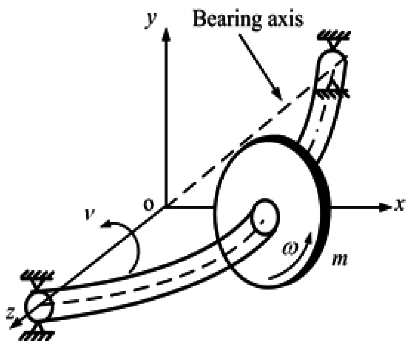
2.3. Rotor-Dynamic Equations

When the external load acting on the rotor or the journal varies both in direction and magnitude, the journal center describes a trajectory within the bearing. The determination of this trajectory requires the solution of the rotor-dynamic equations coupled with those governing the hydrodynamic behavior of lubricating oil films.

Generally, the external loads acting on the rotor are:

-

the weight of the rotor 2W₀ = 2 mg;

-

the dynamic load components $W_X(t)$ and $W_Y(t)$ due an unbalance mass characterized by its eccentricity e;

-

the hydrodynamic forces F_X and F_Y due to the presence of the lubricating oil film.

The rotor-bearings system is modeled as a flexible Jeffcott rotor symmetrically supported by two identical layered hydrodynamics bearings ignoring the gyroscopic effects as depicted in Figure 2. We assume that the rotor mass is lumped at the midpoint with massless shaft, central load of 2m, rotor damping of 2b_r, and rotor stiffness of 2k_r.

For each bearing are attributed a mass m of the rotor, a static applied load W₀ = mg, and a synchronous dynamic excitation due to an unbalance mass $\left|\overrightarrow{W}(t)\right|=me{\omega }^2$.

The application of the dynamic fundamental principle gives

$$\{\begin{array}{l}m\ddot{X}+b_r\dot{X}+k_{r}X=W_0+me{\omega }^2\cos \omega t+F_X(X,Y,\dot{X},\dot{Y})\\ m\ddot{Y}+b_r\dot{Y}+k_{r}Y=me{\omega }^2\sin \omega t+F_Y(X,Y,\dot{X},\dot{Y})\end{array}$$

(25)

where

$$\left\{\begin{array}{c}{F}_X\left(t\right)\\ F_Y\left(t\right)\end{array}\right\}={\displaystyle \underset{-\raisebox{1ex}{$L$}\!\left/ \!\raisebox{-1ex}{$2$}\right.}{\overset{\raisebox{1ex}{$L$}\!\left/ \!\raisebox{-1ex}{$2$}\right.}{\int }}{\displaystyle \underset{0}{\overset{2\pi }{\int }}p\left(\theta ,z,t\right)\left\{\begin{array}{c}\cos \theta \\ \sin \theta \end{array}\right\}Rd\theta dz}}$$

(26)

F_X and F_Y are the hydrodynamic forces in X and Y directions that are nonlinear functions of the displacement components (X,Y) and the velocities $\left(\dot{X},\dot{Y}\right)$ of the journal center O_j. They are calculated by integrating the hydrodynamic pressure over the bearing surface. This latter is obtained by solving the transient modified Reynolds’ equation by finite element method.

In dimensionless variables, Equation (25) is written as

$$\left[\begin{array}{cc}1& 0\\ 0& 1\end{array}\right]\left\{U\prime \prime \right\}+\left[\begin{array}{cc}{B}_r& 0\\ 0& B_r\end{array}\right]\left\{U\prime \right\}+\left[\begin{array}{cc}{K}_r& 0\\ 0& K_r\end{array}\right]\left\{U\right\}=\left\{\begin{array}{c}{W}_0^{*}+\epsilon \cos \left(t^{*}\right)+{\widehat{F}}_X(X^{*},Y^{*},X^{*\prime },Y^{*\prime })\\ \epsilon \sin \left(t^{*}\right)+{\widehat{F}}_Y(X^{*},Y^{*},X^{*\prime },Y^{*\prime }) \end{array}\right\}$$

(27)

where

$$B_r=\frac{b_r}{m\omega } , K_r=\frac{k_r}{m{\omega }^2} , W_0^{*}=\frac{W_0}{mC{\omega }^2}=\frac{g}{C{\omega }^2}, \epsilon =\frac{e}{C} , \left({\widehat{F}}_X, {\widehat{F}}_Y\right)=\frac{{\mu }_0\omega RL{\left(\raisebox{1ex}{$R$}\!\left/ \!\raisebox{-1ex}{$C$}\right.\right)}^2}{mC{\omega }^2} \left(F_X^{*}, F_Y^{*}\right)$$

$$\left\{U\right\}=\left\{\begin{array}{c}{X}^{*}\\ Y^{*}\end{array}\right\}, \left\{U\prime \right\}=\left\{\begin{array}{c}{X}^{*\prime }\\ Y^{*\prime }\end{array}\right\} , \left\{U\prime \prime \right\}=\left\{\begin{array}{c}{X}^{*\prime \prime }\\ Y^{*\prime \prime }\end{array}\right\} , and {(°)}^{\prime }=\frac{d}{d{t}^{*}}(°)=\frac{d(°)}{dt}\frac{dt}{d{t}^{*}}=\frac{1}{\omega }\frac{d}{dt}(°)$$

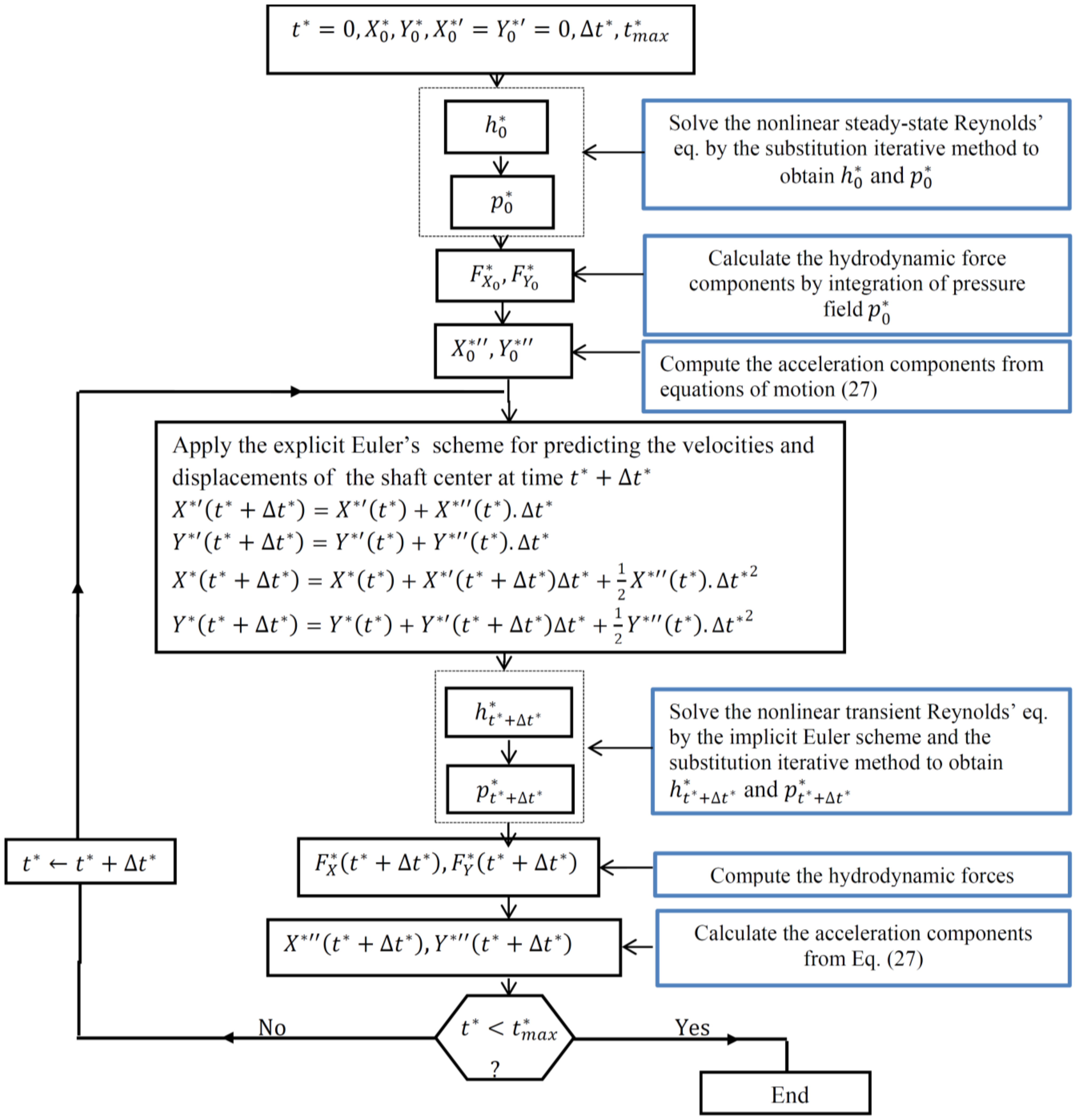
3. Computation Procedure of the Journal Bearing Nonlinear Dynamic Response

Solving the normalized equations of motion (27) ahead of time numerically using the direct integration methods of second order differential equations such as the explicit Euler’s method, the transient motion of the journal center O_j for balanced and unbalanced shafts is determined Figure 4 (See Appendix A for more details).

Figure 4. Flow chart of the computational procedure.

Figure 4. Flow chart of the computational procedure.

4. Finite Element Treatment of the Steady-State Modified Reynolds’ Equation

4.1. Weak Integral Formulation and Finite Element Discretization

In steady-state conditions, the normalized modified Reynolds’ equation becomes

$$\frac{\partial }{\partial \theta }\left(G^{*}\left(h_0^{*},{\ell }^{*}, {\alpha }^{*},p_0^{*}\right)\frac{\partial p_0^{*}}{\partial \theta }\right)+\lambda \frac{\partial }{\partial z^{*}}\left(G^{*}\left(h_0^{*},{\ell }^{*}, {\alpha }^{*},p_0^{*}\right)\frac{\partial p_0^{*}}{\partial z^{*}}\right)=6\frac{\partial h_0^{*}}{\partial \theta }$$

(28a)

where

$$h_0^{*}\left(\theta ,z^{*}\right)=1+X_0^{*}cos\theta +Y_0^{*}sin\theta +\complement {\tilde{p}}_0\left(\theta ,z^{*}\right)$$

(28b)

The Galerkin’s weighted residual method is employed to build up the integral formulation associated to Equation (28a), i.e.,

$$W^{*}\left(p_0^{*}\right)={\displaystyle \underset{D^{*}}{\iint }\delta p_0^{*}\left(\frac{\partial }{\partial \theta }\left(G^{*}\left(h_0^{*},{\ell }^{*},{\alpha }^{*},p_0^{*}\right)\frac{\partial p_0^{*}}{\partial \theta }\right)+\lambda \frac{\partial }{\partial z^{*}}\left(\tilde{G}\left(h_0^{*},{\ell }^{*},{\alpha }^{*},p_0^{*}\right)\frac{\partial p_0^{*}}{\partial z^{*}}\right)-6\frac{\partial h_0^{*}}{\partial \theta }\right)}d{D}^{*}=0$$

(29)

where $\delta p_0^{*}$ is the first variation of $p_0^{*}$, $D^{*}=\left(0,\hspace{0.17em}2\pi \right)\times \left(0,\hspace{0.17em}\raisebox{1ex}{$1$}\!\left/ \!\raisebox{-1ex}{$2$}\right.\right)\subset R^2$ the half computational domain, and $d{D}^{*}=d\theta d{z}^{*}$.

By virtue of Green’s theorem (integration by parts), the weak form of Equation (29) is obtained further. As a result, the weak form contains lower order partial derivatives of $p_0^{*}$ and includes two types of integration. Namely, domain integration over computational domain and contour integration along the boundary of $D^{*}$, i.e., $\partial D^{*}$, the latter can be neglected because $\delta p_0^{*}$ is zero at both ends of the housing, yielding

$$W^{*}\left(p_0^{*}\right)={\displaystyle \underset{D^{*}}{\iint }\left(G^{*}\left(h_0^{*},{\ell }^{*},{\alpha }^{*},p_0^{*}\right)\left(\frac{\partial \delta p_0^{*}}{\partial \theta }\frac{\partial p_0^{*}}{\partial \theta }+\lambda \frac{\partial \delta p_0^{*}}{\partial z^{*}}\frac{\partial p_0^{*}}{\partial z^{*}}\right)-6h_0^{*}\frac{\partial \delta p_0^{*}}{\partial \theta }\right)}d{D}^{*}=0$$

(30)

Isoparametric four-noded rectangular elements with sides parallel to the global axes are used in the discretization of the fluid film domain $D^{*}$ such that $D^{*}={\displaystyle \underset{e\ge 1}{\cup }{D^{*}}^{\left(e\right)}}$.

After writing Equation (30) over a subdomain ${D^{*}}^{\left(e\right)}$and discretisation by the finite element method, we obtain a system of nonlinear algebraic equations

$$W^{*\left(e\right)}\left(p_0^{*\left(e\right)}\right)=\langle \delta p_n\rangle \left(\left[k_e\left(p_0^{*\left(e\right)}\right)\right]\left\{p_0^{*\left(e\right)}\right\}-\left\{f_e\left(p_0^{*\left(e\right)}\right)\right\}\right)$$

(31)

where $\left[k_e\right]$ and $\left\{f_e\right\}$ are the elementary matrices defined as

$$k_{e_{ij}}={\displaystyle \underset{D^{*\left(e\right)}}{\iint }{G}^{*\left(e\right)}}\left(\frac{\partial N_i}{\partial \theta }\frac{\partial N_j}{\partial \theta }+\lambda \frac{\partial N_i}{\partial z^{*}}\frac{\partial N_j}{\partial z^{*}}\right)d\theta d{z}^{*} \mathrm{and} f_{e_i}=6{\displaystyle \underset{D^{*\left(e\right)}}{\iint }{h}_0^{*\left(e\right)}\frac{\partial N_i}{\partial \theta }d\theta d{z}^{*}}$$

(32)

Over the parent element, the bilinear shape functions N_i (Lagrangian polynomials) are expressed as

$$N_i\left(\xi ,\eta \right)=\frac{1}{4}\left(1+{\xi }_i\xi \right)\left(1+{\eta }_i\eta \right); i=1,\hspace{0.17em}2,\hspace{0.17em}3,\hspace{0.17em}4$$

(33)

where $\xi$ and $\eta$ are the local coordinates of an element such that $-1\le \xi ,\eta \le 1$.

Accordingly, static pressure and static film thickness over a parent element are then approached by $p_0^{*\left(e\right)}\left(\xi ,\eta \right)={\displaystyle \sum _{i=1}^4{N}_i\left(\xi ,\eta \right)}{p}_i^{*}$ and $h_0^{*\left(e\right)}\left(\xi ,\eta \right)={\displaystyle \sum _{i=1}^4{N}_i\left(\xi ,\eta \right)}\hspace{0.17em}{h}_i^{*}$, respectively.

The coefficients $k_{e_{ij}} \mathrm{and} f_{e_i}$ are numerically evaluated over the parent element using the Gauss-Legendre quadrature with ($2\times 2$) integration points as depicted in Figure 5.

Figure 5. Representation of integration points over the iso-parametric parent element.

Figure 5. Representation of integration points over the iso-parametric parent element.

After assembling of different elementary matrices, finite element approximation leads to the following nonlinear system:

$$\left[K\left(P_0\right)\right]\left\{P_0\right\}=\left\{F\left(P_0\right)\right\}$$

(34)

where $\left[K\right]=\underset{e\ge 1}{A}\left[k_e\right]$ is the global matrix of fluidity, $\left\{P_0\right\}$ the nodal static pressures vector on the domain (D), and $\left\{F\right\}=\underset{e\ge 1}{A}\left\{f_e\right\}$ the global vector containing the term appearing on the RHS of the stationary modified Reynolds’ equation. $\underset{e\ge 1}{A}$ being the assembling operator.

The static pressure field is integrated over the half bearing domain to generate the dimensionless lift force components, i.e.,

$$\left\{\begin{array}{c}{F}_{X_0}^{*}\\ F_{Y_0}^{*}\end{array}\right\}=2{\displaystyle \sum _{e\ge 1}{\displaystyle \underset{D^{*\left(e\right)}}{\iint }{p}_0^{*\left(e\right)}\left\{\begin{array}{c}\cos {\theta }^{\left(e\right)}\\ \sin {\theta }^{\left(e\right)}\end{array}\right\}}}d\theta d{z}^{*}$$

(35)

with ${\theta }^{\left(e\right)}={\displaystyle \sum _{i=1}^4{N}_i}{\theta }_i$ since the element is isoparametric, i.e., the element geometrical nodes are also the interpolation nodes. The lift force components Equation (35) are also calculated by means of the Gauss-Legendre quadrature with ($2\times 2$) integration points.

4.2. Method of Solution of Steady-State Nonlinear Modified REYNOLDS’ Equation

The steady-state solution of the modified Reynolds’ Equation (28a) which is a highly nonlinear elliptic partial differential equation is obtained by the relaxed substitution iterative method. This method consists of building up a series of solutions $\left\{P_0^{\left(0\right)}\right\}$, $\left\{P_0^{\left(1\right)}\right\}$, ....., $\left\{P_0^{\left(k-1\right)}\right\}$, $\left\{P_0^{\left(k\right)}\right\}$ where $\left\{P_0^{\left(k\right)}\right\}$ being calculated from $\left\{P_0^{\left(k-1\right)}\right\}$ by solving the linear system:

$$\left[K\left(P_0^{\left(k-1\right)}\right)\right]\left\{P_0^{\left(k\right)}\right\}=\left\{F\left(P_0^{\left(k-1\right)}\right)\right\}; k=1, 2, ...., k_{max}$$

(36)

We can write this in incremental form by introducing the residual vector $\left\{R^{\left(k\right)}\right\}$:

$$\left\{R^{\left(k\right)}\right\}=\left\{R\left(P_0^{\left(k-1\right)}\right)\right\}=\left\{F\left(P_0^{\left(k-1\right)}\right)\right\}-\left[K\left(P_0^{\left(k-1\right)}\right)\right]\left\{P_0^{\left(k-1\right)}\right\}$$

(37)

where Ω₀ is an under-relaxation factor which ensures and accelerates the convergence of the iterative process.

To obtain the steady-state fluid pressure, the required steps of the computational procedure are presented in detail in Appendix A.

4.3. Iterative Research of the Steady-State Equilibrium Position

The steady-state equilibrium position of shaft center (X₀,Y₀) due to the application of static load ${\mathit{W}}_0=\left(W_{X0},W_{Y0}\right)$ is determined when the integration of the resulting steady-state hydrodynamic pressure obtained from Equation (28a) balances with the applied load components $\left(W_{X0},W_{Y0}\right)$, i.e.,

$$W_{X_0}^{*}={\displaystyle \underset{-\raisebox{1ex}{$1$}\!\left/ \!\raisebox{-1ex}{$2$}\right.}{\overset{\raisebox{1ex}{$1$}\!\left/ \!\raisebox{-1ex}{$2$}\right.}{\int }}{\displaystyle \underset{0}{\overset{2\pi }{\int }}{p}_0^{*}\cos \theta }}d\theta d{z}^{*}$$

(38a)

$$W_{Y_0}^{*}={\displaystyle \underset{-\raisebox{1ex}{$1$}\!\left/ \!\raisebox{-1ex}{$2$}\right.}{\overset{\raisebox{1ex}{$1$}\!\left/ \!\raisebox{-1ex}{$2$}\right.}{\int }}{\displaystyle \underset{0}{\overset{2\pi }{\int }}{p}_0^{*}\sin \theta }}d\theta d{z}^{*}$$

(38b)

In this case, the bearing load is known as a constant and the position of the shaft center is to be calculated from numerical iterations. Therefore, an inverse solution of the steady-state modified Reynolds’ equation is required (See Appendix A for details).

5. Finite Element Treatment of the Transient Modified Reynolds’ Equation

5.1. Weak Integral Formulation and Finite Element Discretization

Applying the Galerkin weighted residual method and the Green’s theorem, the weak integral form associated to the transient modified Reynolds’ Equation (21) is

$$\underset{-\frac{1}{2}}{\overset{\frac{1}{2}}{{\displaystyle \int }}}\underset{0}{\overset{2\pi }{{\displaystyle \int }}}\left[G^{*}\left(h^{*},{\ell }^{*},{\alpha }^{*},p^{*}\right)\left(\frac{\partial \delta p^{*}}{\partial \theta }\frac{\partial p^{*}}{\partial \theta }+\lambda \frac{\partial \delta p^{*}}{\partial z^{*}}\frac{\partial p^{*}}{\partial z^{*}}\right)-6h^{*}\frac{\partial \delta p^{*}}{\partial \theta }+12\delta p^{*} \frac{\partial h^{*}}{\partial {\mathrm{t}}^{*}}\right]d{D}^{*}=0$$

(39)

where

$$\frac{\partial h^{*}}{\partial \tilde{t}}={h^{*}}^{\prime }=X^{*\prime }cos\theta +Y^{*\prime }sin\theta +\complement p^{*\prime }$$

(40)

According to Equation (40), Equation (39) becomes:

$$\underset{-\frac{1}{2}}{\overset{\frac{1}{2}}{{\displaystyle \int }}}\underset{0}{\overset{2\pi }{{\displaystyle \int }}}{G}^{*}\left(h^{*},{\ell }^{*},{\alpha }^{*},p^{*}\right)\left(\frac{\partial \delta p^{*}}{\partial \theta }\frac{\partial p^{*}}{\partial \theta }+\lambda \frac{\partial \delta p^{*}}{\partial z^{*}}\frac{\partial p^{*}}{\partial z^{*}}\right)d\theta d{z}^{*}+\underset{-\frac{1}{2}}{\overset{\frac{1}{2}}{{\displaystyle \int }}}\underset{0}{\overset{2\pi }{{\displaystyle \int }}}12\delta p^{*}\complement p^{*\prime }d\theta d{z}^{*}=6\underset{-\frac{1}{2}}{\overset{\frac{1}{2}}{{\displaystyle \int }}}\underset{0}{\overset{2\pi }{{\displaystyle \int }}} h^{*}\frac{\partial \delta p^{*}}{\partial \theta }d\theta d{z}^{*}-12\underset{-\frac{1}{2}}{\overset{\frac{1}{2}}{{\displaystyle \int }}}\underset{0}{\overset{2\pi }{{\displaystyle \int }}}\delta p^{*}(X^{*\prime }cos\theta +Y^{*\prime }sin\theta )d\theta d{z}^{*}$$

(41)

After writing Equation (41) over a subdomain ${D^{*}}^{\left(e\right)}$and discretisation by the finite element method, we obtain a set of first order differential equations

$$\left[c_e\right]\left\{p{\prime }_n\right\}+\left[k_e\right]\left\{p_n\right\}= \left\{f_e\right\}$$

(42)

where

$$\left[c_e\right]= 12{\int }^{}{\int }_{{D^{*}}^{\left(e\right)}}^{ }\complement \left\{N\right\}<N>d{D^{*}}^{\left(e\right)} \mathrm{or} {c_e}_{ij}= 12{\int }^{}{\int }_{{D^{*}}^{\left(e\right)}}^{ }\complement N_i{N}_{j}d{D^{*}}^{\left(e\right)}$$

$$\left[k_e\right]= {{\displaystyle \int }}^{}{{\displaystyle \int }}_{{D^{*}}^{\left(e\right)}}^{ }{G}^{*\left(e\right)} \left(\left\{\frac{\partial N}{\partial \theta }\right\}<\frac{\partial N}{\partial \theta }>+\lambda \left\{\frac{\partial N}{\partial z^{*}}\right\}<\frac{\partial N}{\partial z^{*}}>\right)d{D^{*}}^{\left(e\right)}$$

or

$${k_e}_{ij}={{\displaystyle \int }}^{}{{\displaystyle \int }}_{{D^{*}}^{\left(e\right)}}^{ }{G}^{*\left(e\right)} \left(\frac{\partial N_i}{\partial \theta }\frac{\partial N_j}{\partial \theta }+\lambda \frac{\partial N_i}{\partial z^{*}}\frac{\partial N_j}{\partial z^{*}}\right)d{D^{*}}^{\left(e\right)}$$

$$\left\{f_e\right\}= 12{{\displaystyle \int }}^{}{{\displaystyle \int }}_{{D^{*}}^{\left(e\right)}}^{ }\left(\frac{h^{*\left(e\right)}}{2}\left\{\frac{\partial N}{\partial \theta }\right\}-\left(X^{*\prime }cos\theta +Y^{*\prime }sin\theta \right)\left\{N\right\}\right)d{D^{*}}^{\left(e\right)}$$

or

$${f_e}_i=12{{\displaystyle \int }}^{}{{\displaystyle \int }}_{{D^{*}}^{\left(e\right)}}^{ }\left(\frac{h^{*\left(e\right)}}{2}\frac{\partial N_i}{\partial \theta }-\left(X^{*\prime }cos\theta +Y^{*\prime }sin\theta \right)N_i\right)d{D^{*}}^{\left(e\right)}$$

After assembling of elementary matrices, we get

$$\left[C\left(P_{t^{*}}\right)\right]\left\{P_{t^{*}}^{\prime }\right\}+\left[K\left(P_{t^{*}}\right)\right]\left\{P_{t^{*}}\right\}= \left\{F\left(P_{t^{*}}\right)\right\}$$

(43)

5.2. Method of Solution of Transient Nonlinear Modified Reynolds’ Equation

We found in the preceding section that solving the modified Reynolds’ equation under dynamic conditions by the finite element reduces ultimately to the solution of simultaneous nonlinear first order ordinary differential equations of the form Equation (43).

After formation of matrix Equation (43) the matrices must be restructured or modified to account for any essential boundary conditions Equation (24). In addition to the boundary conditions, we must also know the initial conditions, i.e., $\left\{P\left(0\right)\right\}$. There are many general methods and several special techniques for solving first-order matrix differential equations. We consider the direct numerical integration in time to solve the original set of coupled equations. The procedure relies on deriving recursion formulas that relate the values of $\left\{P\right\}$ at one instant of dimensionless time $\tilde{t}$ to the values of $\left\{P\right\}$ at a later time $\tilde{t}+∆\tilde{t}$, where $∆\tilde{t}$ is the dimensionless time step. The recursion formulas make it possible for the solution to be marched out in time, starting from the initial conditions at time $\tilde{t}=0$ and continuing step by step until reaching the desired duration.

Consider the semi-implicit Euler method for solving Equations (43). We write these equations at time ${\mathrm{t}}_{\beta }^{*}=t^{*}+\beta ∆t^{*}$, where$0\le \beta \le 1$ as

$${\left[\complement \left(P\right)\right]}_{{\mathrm{t}}_{\beta }^{*}}{\left\{P^{\prime }\right\}}_{{\mathrm{t}}_{\beta }^{*}}+{\left[K\left(P\right)\right]}_{{\mathrm{t}}_{\beta }^{*}}{\left\{P\right\}}_{{\mathrm{t}}_{\beta }^{*}}= {\left\{F\left(P\right)\right\}}_{{\mathrm{t}}_{\beta }^{*}}$$

(44)

and introduce the following approximations

$${\left\{P^{\prime }\right\}}_{{\mathrm{t}}_{\beta }^{*}}=\frac{{\left\{P\right\}}_{t^{*}+∆t^{*}}-{\left\{P\right\}}_{t^{*}}}{∆t^{*}}$$

(45a)

$${\left\{P\right\}}_{{\mathrm{t}}_{\beta }^{*}}=\left(1-\beta \right){\left\{P\right\}}_{t^{*}}+\beta {\left\{P\right\}}_{t^{*}+∆t^{*}}$$

(45b)

$${\left\{F\left(P\right)\right\}}_{{\mathrm{t}}_{\beta }^{*}}=\left(1-\beta \right){\left\{F\left(P\right)\right\}}_{t^{*}}+\beta {\left\{F\left(P\right)\right\}}_{t^{*}+∆t^{*}}$$

(45c)

Substituting Equation (45a) to (45c) into Equation (44) gives

$$\left[\overline{K}\left(P\right)\right]{\left\{P\right\}}_{t^{*}+∆t^{*}}= {\left\{\overline{F}\left(P\right)\right\}}_{t^{*}+∆t^{*}}$$

(46)

where $\left[\overline{K}\right]= \frac{1}{∆t^{*}}\left[C\left(P\right)\right]+ \beta \left[K\left(P\right)\right]$

and

$$\left\{{\overline{F}}_{t^{*}+∆t^{*}}\right\}=\left(\frac{1}{∆t^{*}}\left[C\left(P\right)\right]-\left(1-\beta \right) \left[K\left(P\right)\right]\right){\left\{P\right\}}_{t^{*}}+\left(1-\beta \right){\left\{F\left(P\right)\right\}}_{t^{*}}+\beta {\left\{F\left(P\right)\right\}}_{t^{*}+∆t^{*}}$$

where the ${\left\{P\right\}}_{t^{*}+∆t^{*}}$ on the left-hand side of the equation are unknowns, and all of the terms on the right-hand side are known. Equation (46) represents a general family of recurrence relations. If β = 0, we get the explicit Euler algorithm, i.e.,

$$\frac{1}{∆t^{*}}\left[C\left(P\right)\right]{\left\{P\right\}}_{t^{*}+∆t^{*}}=\left(\frac{1}{∆t^{*}}\left[C\left(P\right)\right]- \left[K\left(P\right)\right]\right){\left\{P\right\}}_{t^{*}}+{\left\{F\left(P\right)\right\}}_{t^{*}}$$

(47)

and if β = 1 we obtain the implicit Euler method

$$\left(\frac{1}{∆t^{*}}\left[C\left(P\right)\right]+ \left[K\left(P\right)\right]\right){\left\{P\right\}}_{t^{*}+∆t^{*}}=\frac{1}{∆t^{*}}\left[C\left(P\right)\right]{\left\{P\right\}}_{t^{*}}+{\left\{F\left(P\right)\right\}}_{t^{*}+∆t^{*}}$$

(48)

If $\left[C\right]=0 and X^{\prime }=Y^{\prime }=0$, we get the nonlinear algorithm for the steady-state modified Reynolds’ Equation.

6. Results and Discussions

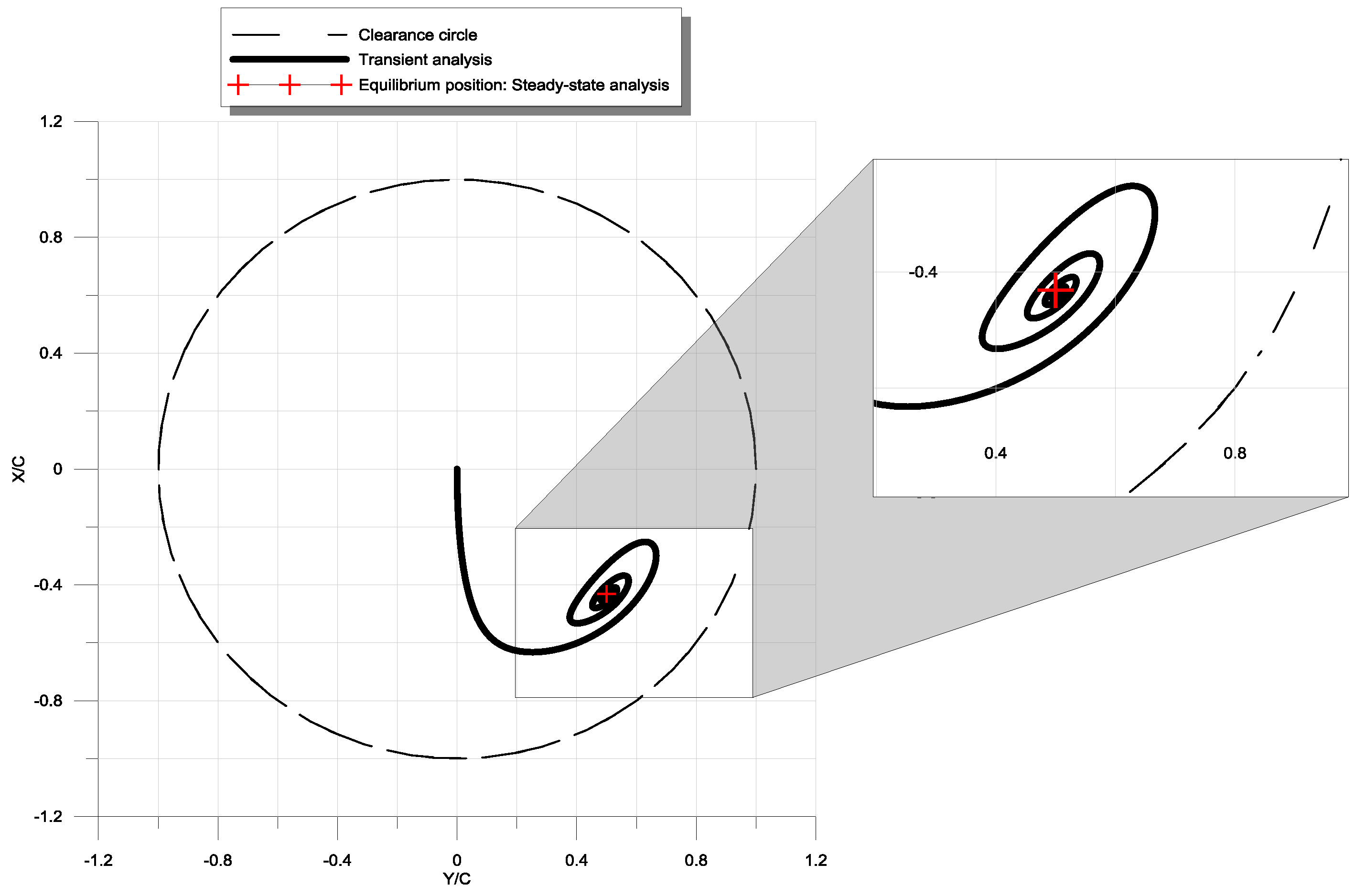
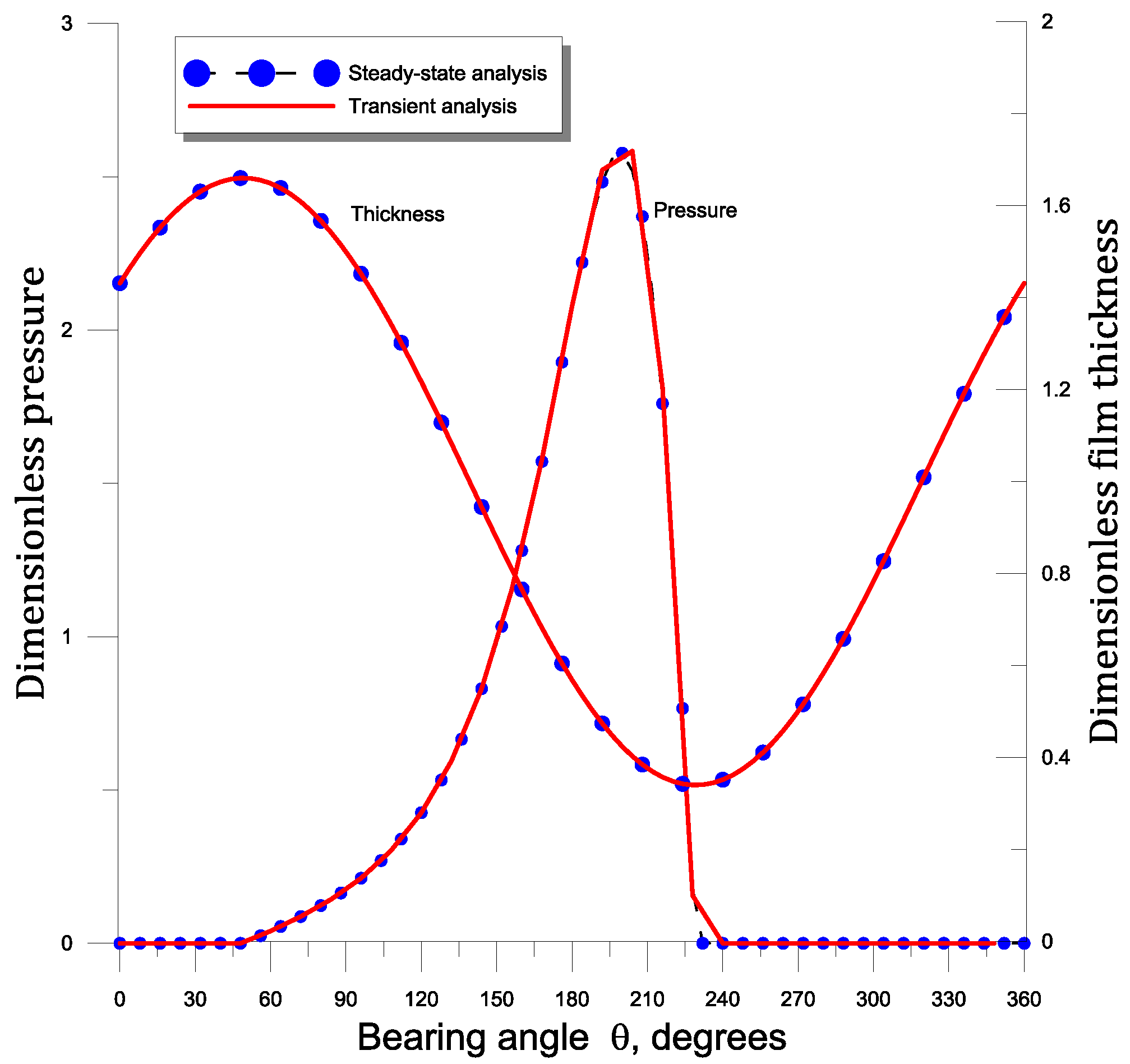
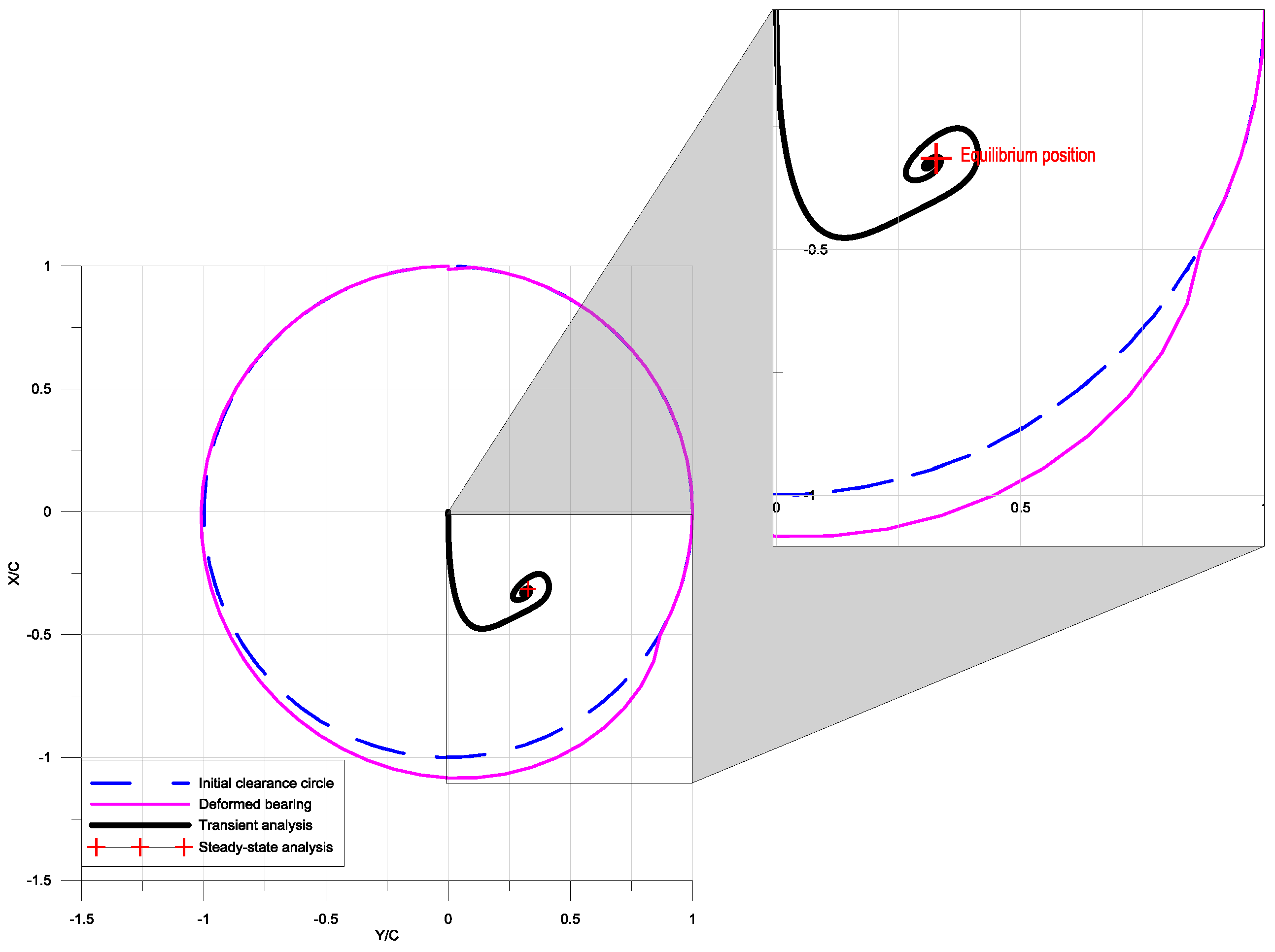
6.1. Transient Solution vs. Steady-State Solution

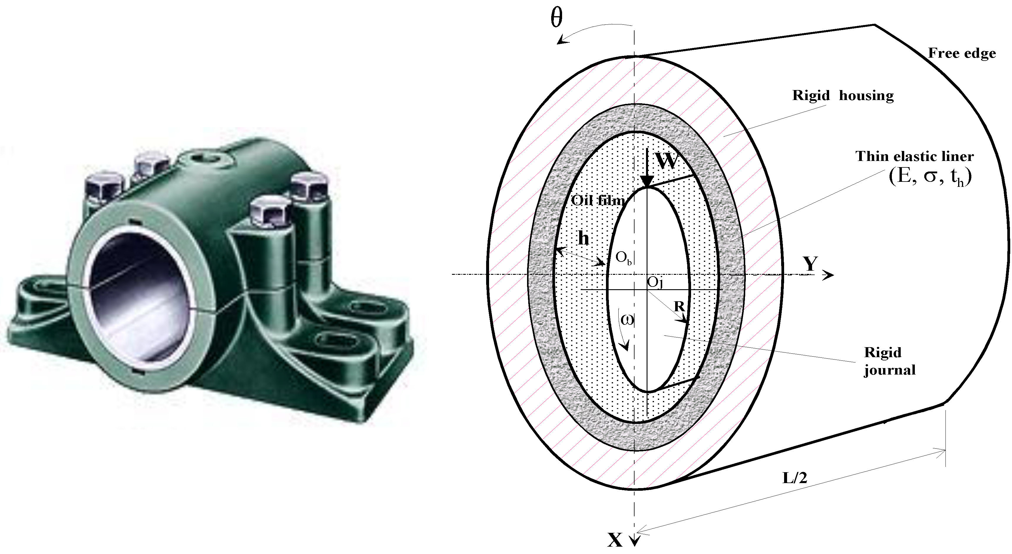
The nonlinear dynamic analysis, described in the Section 5, has been incorporated into a computer program.

In order to check the correctness of the results obtained from the nonlinear transient analysis of hydrodynamic journal bearings, a separate 2-D finite difference computer program was developed to calculate the steady-state position by solving the inverse hydrodynamic lubrication by means of the relaxed iterative Newton-Raphson method as stated in Section 4. For (2-D) finite difference analysis, which in this paper will be referred to as the exact solution, a grid size of (61 × 16) nodes is used in θ and z directions, respectively. The number of nodes is chosen in order to ensure accurate results with minimum CPU time. The rotor and bearing parameter values used in the calculations as well as the finite element meshing characteristics and data of calculations are reported in Table 1 and Table 2. In this section, the calculations were made for two different cases:

Case 1: A balanced rigid journal bearing lubricated with Newtonian and iso-viscous lubricant: W₀ = 340 kN (S = 0.18, $W_0^{*}$ = 1.8), α^* = 0, ℓ^* = 0, C_d = 0, ε = 0.

Case 2: A balanced layered journal bearing lubricated with piezo-viscous couple stress lubricant: W₀ = 2720 kN (S = 0.0225, $W_0^{*}$ = 14), α = 17 × 10⁻⁹ Pa⁻¹, ε = 0, ℓ^* = 0.3, t_h = 10 × 10⁻³ m, E = 0.9 GPa, σ = 0.35.

For both cases, the geometrical characteristics such as the bearing length, the bearing radius and the radial clearance as well as the rotational velocity are the same and are given in Table 1.

Table 1. Rotor and bearing parameter values used in the calculations.

Parameter	Symbol	Unit	Value
Bearing length	L	m	0.320
Journal diameter	D = 2R	m	0.500
Radial clearance	C	m	3.5 × 10−4
Bearing-liner thickness	$t_h$	m	10−2
Young’s modulus of the bearing-liner (polyethylene high density at 20 °C) [41]	E	Pa	0.9 × 109
Poisson’s ratio of the bearing-liner at 20 °C [41]	σ	-	0.35
Dynamic viscosity of lubricant at atmospheric pressure	${\mu }_0$	Pa·s	15 × 10−3
Density of lubricant	ρ	kg·m−3	870
Pressure-viscosity coefficients	α	Pa−1	0
			17 × 10−9
			42.5 × 10−9
			212.5 × 10−9
Rotor speed	$N$	rpm	3 × 103
Rotor mass (disc)	2m	kg	68 × 103
Rotor length	Lr	m	10
Young’s modulus of the rotor (steel) at 20 °C	Er	Pa	210 × 109
Rotor stiffness	kr	N/m	5 × 106
Rotor damping	br	N·s/m	0
Mass unbalance eccentricities	e	m	0
			70 × 10−6
			280 × 10−6
Unbalance dynamic loads	meω2	kN	0 235 940
Static load applied per bearing	W0 = mg	kN	340

Table 1. Rotor and bearing parameter values used in the calculations.

Parameter	Symbol	Unit	Value
Bearing length	L	m	0.320
Journal diameter	D = 2R	m	0.500
Radial clearance	C	m	3.5 × 10−4
Bearing-liner thickness	$t_h$	m	10−2
Young’s modulus of the bearing-liner (polyethylene high density at 20 °C) [41]	E	Pa	0.9 × 109
Poisson’s ratio of the bearing-liner at 20 °C [41]	σ	-	0.35
Dynamic viscosity of lubricant at atmospheric pressure	${\mu }_0$	Pa·s	15 × 10−3
Density of lubricant	ρ	kg·m−3	870
Pressure-viscosity coefficients	α	Pa−1	0
			17 × 10−9
			42.5 × 10−9
			212.5 × 10−9
Rotor speed	$N$	rpm	3 × 103
Rotor mass (disc)	2m	kg	68 × 103
Rotor length	Lr	m	10
Young’s modulus of the rotor (steel) at 20 °C	Er	Pa	210 × 109
Rotor stiffness	kr	N/m	5 × 106
Rotor damping	br	N·s/m	0
Mass unbalance eccentricities	e	m	0
			70 × 10−6
			280 × 10−6
Unbalance dynamic loads	meω2	kN	0 235 940
Static load applied per bearing	W0 = mg	kN	340

Figure 6 shows the shaft center trajectory obtained using the transient analysis in the case 1, i.e., when the bearing is rigid and the lubricant is Newtonian. We can notice in this case that this trajectory tends to reach the shaft equilibrium position obtained from the steady state analysis which locates at ($X_0^{*}$ = 0.431287,$Y_0^{*}$ = 0.499599). These values are almost close to those predicted by the transient analysis which are (X^* = 0.439241, Y^* = 0.501445).

Figure 6. Journal center trajectory and final position for the case 1 (W₀ = 340 kN ($W_0^{*}$ = 1.8), S = 0.18, α^* = 0, ℓ^* = 0, C_d = 0, ε = 0).

Figure 6. Journal center trajectory and final position for the case 1 (W₀ = 340 kN ($W_0^{*}$ = 1.8), S = 0.18, α^* = 0, ℓ^* = 0, C_d = 0, ε = 0).

In Figure 7, we represent a comparison of film thickness and pressure profile obtained by the transient and steady state methods in the case 1. A very good agreement is observed.

Figure 7. Comparison of steady-state oil-film pressure and film thickness curves calculated from steady-state and transient analysis. (W₀ = 340 kN ($W_0^{*}$ = 1.8), S = 0.18, α^* = 0, ℓ^* = 0 C_d = 0, ε = 0).

Figure 7. Comparison of steady-state oil-film pressure and film thickness curves calculated from steady-state and transient analysis. (W₀ = 340 kN ($W_0^{*}$ = 1.8), S = 0.18, α^* = 0, ℓ^* = 0 C_d = 0, ε = 0).

Figure 8 depicts the shaft center trajectory calculated with the transient analysis in the case 2, i.e., when considering the compliance of the bearing-liner and the lubricant as a non-Newtonian couple stress fluid. Similar trends for case 2 are obtained as in case 1, i.e., the path of shaft center gradually approaches the static equilibrium position whose the co-ordinates are ($X_0^{*}$ = 0.3143, $Y_0^{*}$ = 0.3268). The values predicted by the transient analysis are (X^* = 0.3272, Y^* = 0.3136). As in the case 1, the discrepancy between the two results is very small.

Figure 8. Journal center trajectory and final position for the case 2. (W₀ = 2720 kN ($W_0^{*}$ = 14.14), S = 0.0225, α = 17 × 10⁻⁹ Pa⁻¹, ε = 0, ℓ^* = 0.3, t_h = 10 × 10⁻³ m, E = 0.9 GPa, σ = 0.35).

Figure 8. Journal center trajectory and final position for the case 2. (W₀ = 2720 kN ($W_0^{*}$ = 14.14), S = 0.0225, α = 17 × 10⁻⁹ Pa⁻¹, ε = 0, ℓ^* = 0.3, t_h = 10 × 10⁻³ m, E = 0.9 GPa, σ = 0.35).

Figure 9 and Figure 10 illustrate the differences between the results for a rigid bearing lubricated with an iso-viscous Newtonian fluid and for a compliant bearing using a piezo-viscous polar fluid as lubricant.

Figure 9. Comparison of nonlinear unbalanced shaft center trajectories for flexible rotor and large unbalance mass (ε = 0.80).

Figure 9. Comparison of nonlinear unbalanced shaft center trajectories for flexible rotor and large unbalance mass (ε = 0.80).

Figure 10. Comparison of nonlinear unbalanced shaft center trajectories for flexible rotor and small unbalance mass (ε = 0.20).

Figure 10. Comparison of nonlinear unbalanced shaft center trajectories for flexible rotor and small unbalance mass (ε = 0.20).

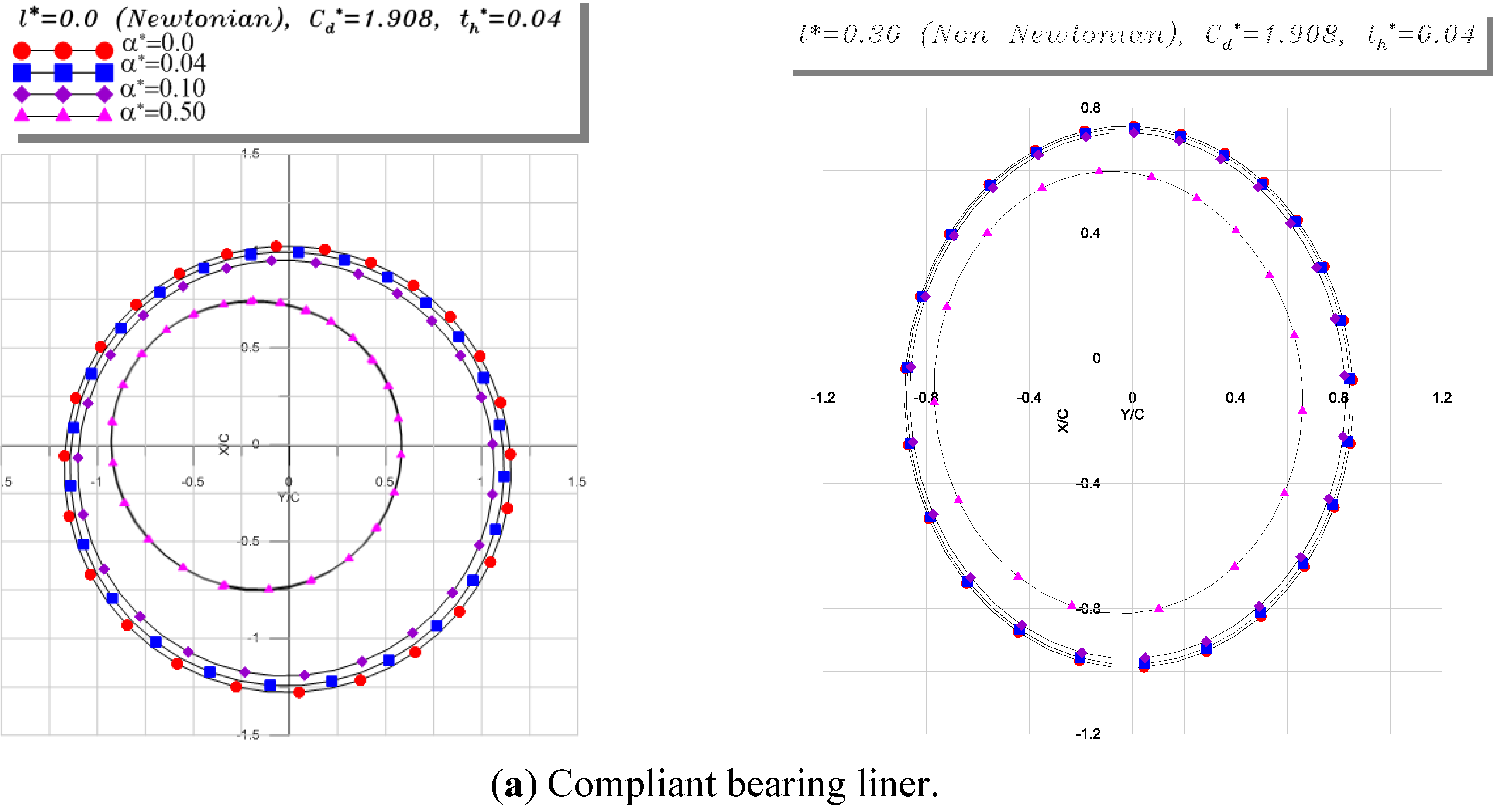
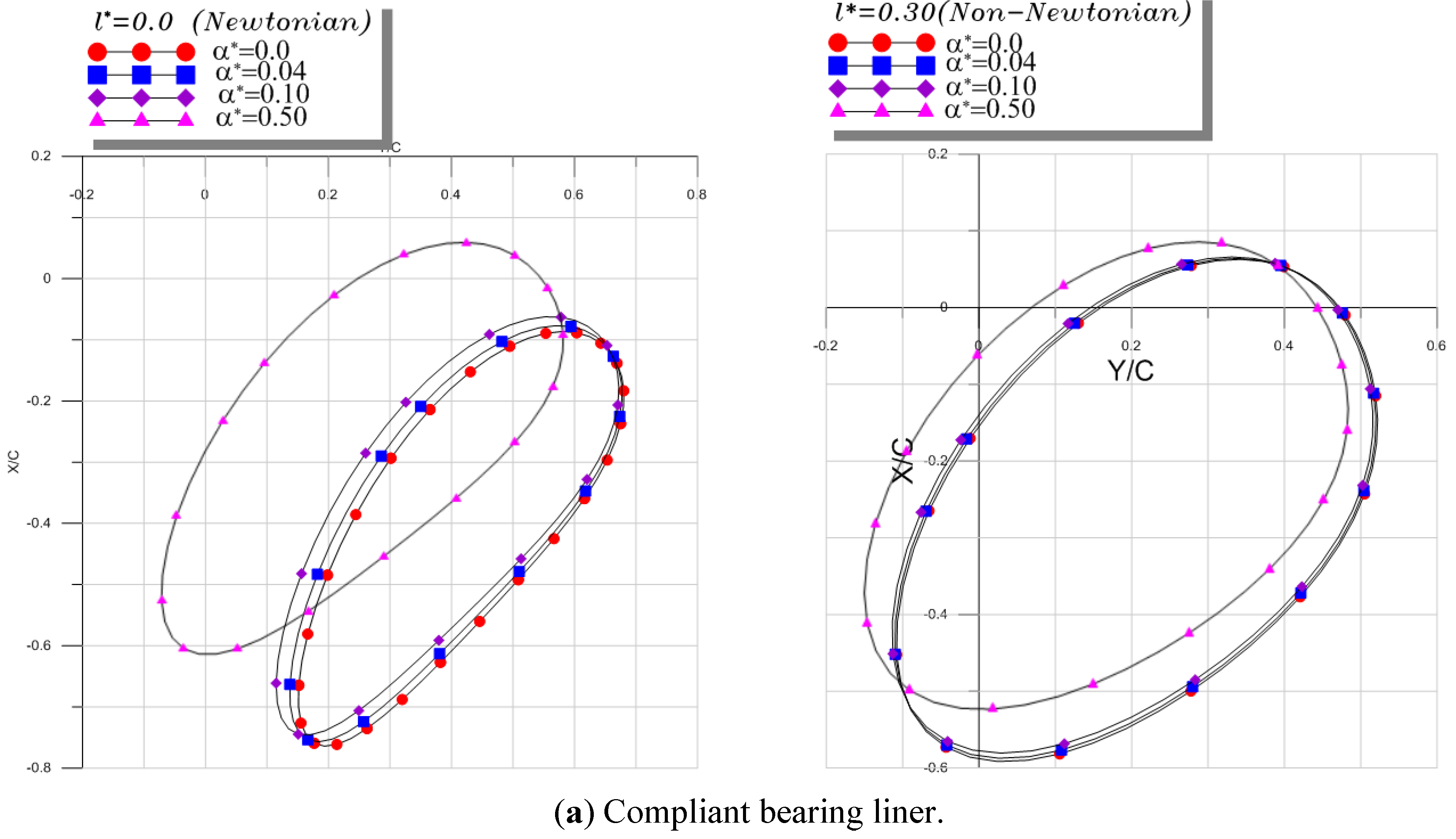
6.2. Parametric Study

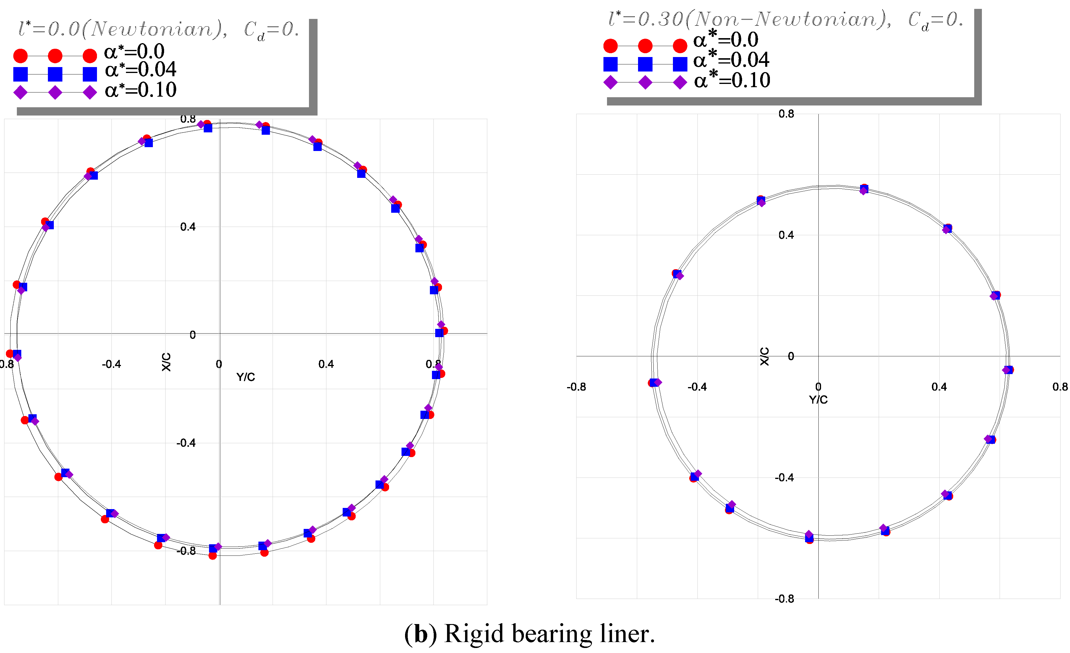
6.2.1. Flexible Rotor with Large Unbalance Mass

Figure 9 represents the trajectories of the shaft center in given running conditions:

W₀ = 340 kN, t_h = 10⁻² m, E = 0.9 GPa, σ = 0.35, b_r = 0, k_r = 5 MN/m, N = 3000 rpm or ω = 100 × π rad/s, and ε = 0.80. Note that for the rigid bearing-liner, the Young’s modulus of liner E tends to infinity and the deformation coefficient $C_d$ is then equal to zero because it is inversely proportional to the elasticity modulus.

The relative unbalance eccentricity ε = 0.80 corresponding to e = 280 microns generates a dynamic load W = meω² = 940 kN at synchronous frequency (ν/ω = 1). For this operating condition, the value of W is greater than the static load W₀ (W/W₀ ≈ 3) and is representative of some emergency conditions in turbomachinery when a blade is lost for example.

It is noted that only the final form of shaft center orbits will be presented in the following, i.e., the results corresponding to the transient numerical effect due to initial conditions will be omitted.

The trajectories of the shaft center within the compliant bearing $\left(C_d^{*}=1.908, \sigma =0.35 and t_h^{*}=0.04\right)$ are given in Figure 9a for two values of couple stress parameter l^* = 0.0 (Newtonian case) and l^* = 0.0 (non-Newtonian couple stress fluid), and different values of the piezo-viscosity coefficient ranging from 0.0 (iso-viscous case) to 0.50. In these operating conditions, the rotor has a very large amplitude of circular or pseudo-circular motion and the nonlinear dynamic behavior appears clearly. This is due to the fact that the dynamic loading due to a large unbalance mass is very important compared to the static one as afore-mentioned above.

On the other hand, we observe in the Newtonian case l^* = 0 that increasing the pressure coefficient α^* shorten the shaft trajectories. This is due to the pressure rise leading to a higher load carrying capacity which reacts and reduces the trajectories size. We can notice that the operating eccentricity of the journal bearing can be greater than the radial clearance in this case where the unbalance mass is large. Furthermore, the orbits described by the shaft center are widely modified by the bearing compliance especially for the non-Newtonian case as clearly illustrated in Figure 9a. They exactly follow the shape of the deformed bearing.

Figure 9b represents the case of rigid bearing-liner. It is seen that the influence of pressure viscosity α^* on the orbits is weak in both Newtonian and non-Newtonian cases. That means in this case the distortion plays a major role in the bearing response. Moreover, the non-Newtonian orbits are smaller than those obtained in the Newtonian case, i.e., when the couple stress parameter l^* of the lubricating fluid increases.

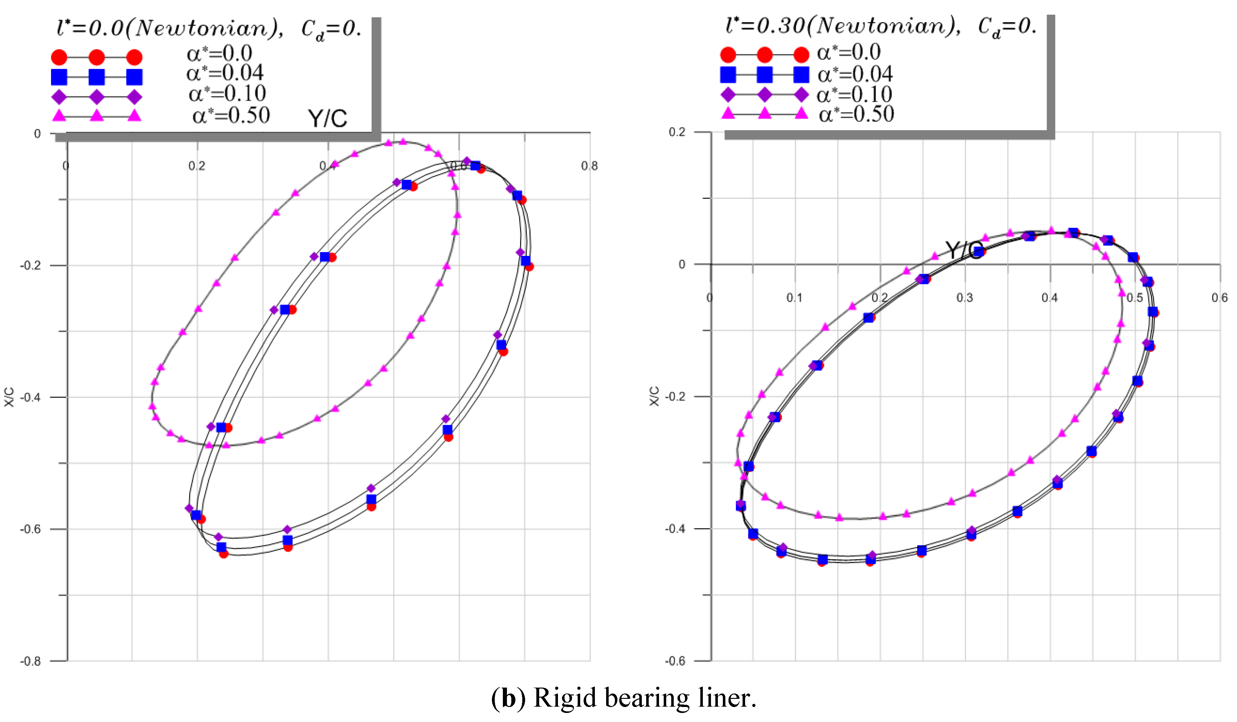
6.2.2. Flexible Rotor with Small Unbalance Mass

The relative unbalance eccentricity ε = 0.20 corresponding to e = 70 microns generates a dynamic load W = meω² = 235 kN at synchronous frequency (ν/ω= 1) which corresponds to 0.70 times the static load. This defect may be attributed to a large residual unbalance which could exist in the shaft.

The trajectories of the shaft center within the rigid and compliant bearings are given in Figure 10 for the same values of the couple stress parameter l^* and the piezo-viscosity coefficient. As expected, the shaft center moves around the equilibrium position in both cases since the dynamic load is smaller than the static one. Moreover, the co-ordinates of the equilibrium position change when increasing the piezo-viscosity coefficient especially for higher values of this coefficient in both Newtonian and non-Newtonian cases. So, it results a shift of orbits towards the bearing center as depicted in the figure.

For small unbalance value as the pressure magnitude is lower the impact of bush distortion is less pronounced than for a large unbalanced case.

For the rigid case, we observe in Figure 10b the same tendencies with smaller size trajectories.

Table 2. Finite element meshing characteristics and data of calculations.

Parameter	Symbol	Value
Number of elements in the circumferential direction of bearing	Nθ	30
Number of elements in the axial direction of half-bearing	Nz	10
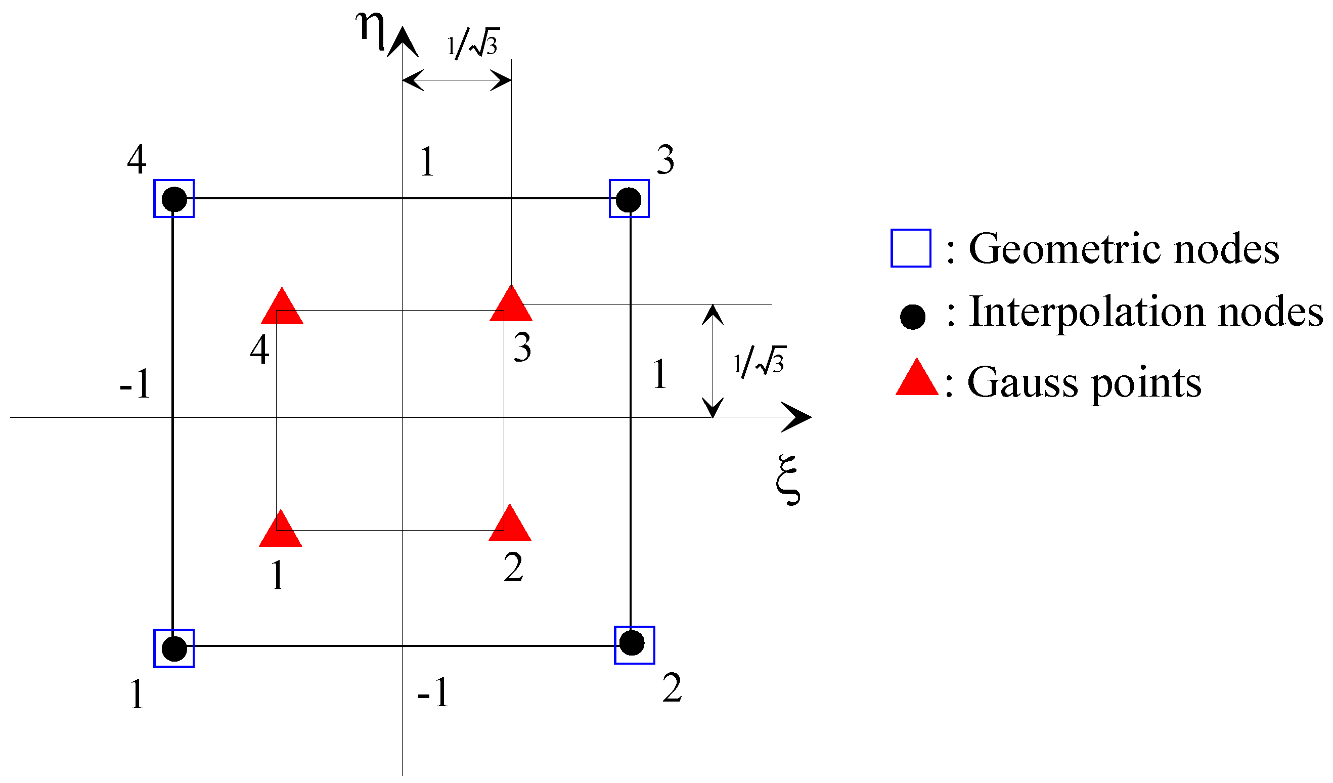
Number of Gauss integration points in ξ-direction	-	2
Number of Gauss integration points in η-direction		2
Under-relaxation factor for the substitution iterative method	Ω0	0.10
Convergence criterion of the substitution iterative method	εp	10−5
Dimensionless time increment	Δ$t^{*}=\omega ∆t$	$2\pi /50$
Time limit	${t^{*}}_{max}$	40π †

^† This value corresponds to 20 revolutions of the shaft.

Table 2. Finite element meshing characteristics and data of calculations.

Parameter	Symbol	Value
Number of elements in the circumferential direction of bearing	Nθ	30
Number of elements in the axial direction of half-bearing	Nz	10
Number of Gauss integration points in ξ-direction	-	2
Number of Gauss integration points in η-direction		2
Under-relaxation factor for the substitution iterative method	Ω0	0.10
Convergence criterion of the substitution iterative method	εp	10−5
Dimensionless time increment	Δ$t^{*}=\omega ∆t$	$2\pi /50$
Time limit	${t^{*}}_{max}$	40π †

^† This value corresponds to 20 revolutions of the shaft.

7. Conclusions

In this paper, a transient nonlinear analysis was developed and presented with details to investigate the nonlinear dynamic response of an unbalanced Jeffcott flexible rotor mounted in layered journal bearings lubricated with a piezo-viscous polar fluid. The analysis is based on the V. K. Stokes micro-continuum theory for describing the flow of piezo-viscous polar lubricants blended with additives. Using the classical assumptions of hydrodynamic lubrication, a transient and nonlinear modified Reynolds equation was derived in order to take into consideration the combined effects of pressure dependent viscosity and couple stresses resulting from the presence of polymer additives in the base oil. The trajectories of the shaft center were obtained numerically by solving the rotordynamics equations with the explicit Euler’s scheme.

The two dominant parameters in the present analysis are the viscosity-pressure coefficient and the couple stress parameter. Such parameters must be considered as key parameters to design adequately bearings of rotating machineries.

The obtained results have been compared with the iso-viscous and Newtonian case.

According to the theoretical results presented, the combined effects of couple stresses due to the presence of polymer additives in lubricant and the pressure dependent viscosity provide lift load enhancement and produce higher oil-film thickness and more contracted trajectories of the shaft center even at severe running conditions (e.g., higher loading, large unbalance mass, etc.). In these circumstances, the destructive metal-to-metal contact between the shaft and bearing surfaces may also be avoided because of the elasticity of the bearing. Qualitatively, these results agree very well with those obtained by the same authors [33] in the case of internal combustion engine connecting-rod bearings lubricated with an iso-viscous polar fluid.

References

1. Newkirk, B.L. Shaft whipping. Gen. Electr. Rev. 1924, 27, 169–178. [Google Scholar]
2. Newkirk, B.L.; Taylor, H.D. Shaft whipping due to oil action in journal bearings. Gen. Electr. Rev. 1925, 28, 985–988. [Google Scholar]
3. Stodola, A. Kritische Wellenstörung Infolge der Nachgiebigkeit des Oelpolsters im Lager. Schweizerische Bauzeitung 1925, 85/86. [Google Scholar] [CrossRef]
4. Hummel, B.L. Kritische Drehzahlen als folge der Nachgiebigkeit des Schmiermittels im Lager. A.W. Zickfeldt: Berlin, Germany, 1926. [Google Scholar]
5. Newkirk, B.L. Whirling balance shafts. In Proceedings of the Third ICAM, Stockholm, Sweden; 1931. [Google Scholar]
6. Hori, Y. A theory of oil whip. ASME J. Appl. Mech. 1959, 81, 189–198. [Google Scholar]
7. Sternlicht, B. Elastic and damping properties of cylindrical journal bearings. J. Basic Eng. 1959, 81, 101–108. [Google Scholar]
8. Holmes, R. The vibration of a rigid shaft on short sleeve bearings. J. Mech. Eng. Sci. 1960, 2, 337–341. [Google Scholar] [CrossRef]
9. Lund, J.W. The stability of an elastic rotor in journal bearings with flexible damped supports. ASME J. Appl. Mech. 1965, 32, 911–920. [Google Scholar] [CrossRef]
10. Lund, J.W.; Saibel, E. Oil whip orbits of a rotor in sleeve bearings. ASME J. Eng. Ind. 1967, 89, 813–823. [Google Scholar] [CrossRef]
11. Badgley, H.; Booker, J.F. Turbo-rotor instability: Effect of initial transients on plain motion. ASME J. Lubr. Technol. 1969, 91, 625–633. [Google Scholar] [CrossRef]
12. Akers, A.; Michaelson, S.; Cameron, A. Stability contours for a whirling finite journal bearing. ASME J. Lubr. Technol. 1971, 93, 177–190. [Google Scholar] [CrossRef]
13. Kirk, R.G.; Gunter, E.J. Short bearing analysis applied to rotor dynamics. Part 1: Theory. ASME J. Lubr. Technol. 1976, 98, 47–56. [Google Scholar] [CrossRef]
14. Kirk, R.G.; Gunter, E.J. Short bearing analysis applied to rotor dynamics. Part 2: Results of journal bearing response. ASME J. Lubr. Technol. 1976, 98, 319–329. [Google Scholar] [CrossRef]
15. Hahn, E.J. Stability and unbalance response of centrally preloaded rotors mounted in journal and squeeze film bearings. ASME J. Lubr. Tech. 1979, 101, 120–128. [Google Scholar] [CrossRef]
16. Grosby, W.A. The stability of a rigid rotor in ruptured finite journal bearings. Wear 1982, 80, 333–346. [Google Scholar] [CrossRef]
17. Akkok, M.; Ettles, C.M. Journal bearing response to excitation and behavior in the unstable region. ASLE Trans. 1984, 27, 341–351. [Google Scholar] [CrossRef]
18. Lahmar, M.; Haddad, A.; Nicolas, D. An optimized short bearing theory for nonlinear dynamic analysis of turbulent journal bearings. Eur. J. Mech. A/Solids 2000, 19, 151–177. [Google Scholar] [CrossRef]
19. Agnieszka (Agnes) Muszyǹska, Rotodynamics; Taylor & Francis: New York, USA, 2005.
20. Laha, S.K.; Kakoty, S.K. Non-linear dynamic analysis of a flexible rotor supported on porous oil journal bearings. Commun. Nonlinear Sci. Numer. Simulat. 2011, 16, 1617–1631. [Google Scholar] [CrossRef]
21. Kushare, P.B.; Sharma, S.C. Nonlinear transient stability study of two lobe symmetric hole entry worn hybrid journal bearing operating with non-Newtonian lubricant. Tribol. Int. 2014, 69, 84–101. [Google Scholar] [CrossRef]
22. Oliver, D.R. Load enhancement effects due to polymer thickening in a short model journal bearings. J. Non-Newton. Fluid Mech. 1988, 30, 185–196. [Google Scholar] [CrossRef]
23. Spikes, H.A. The behaviour of lubricants in contacts: Current understanding and future possibilities. J. Eng Tribol. Proc. IMechE 1994, 28, 3–15. [Google Scholar] [CrossRef]
24. Ariman, T.T.; Sylvester, N.D. Microcontinuum fluid mechanics: A review. Int. J. Eng. Sci. 1973, 11, 905–930. [Google Scholar] [CrossRef]
25. Ariman, T.T.; Sylvester, N.D. Application of microcontinuum fluid mechanics. J. Eng. Sci. 1974, 12, 273–293. [Google Scholar] [CrossRef]
26. Stokes, V.K. Couple-stresses in fluids. Phys. Fluids 1966, 9, 1709–1715. [Google Scholar] [CrossRef]
27. Lin, J.R. Static and dynamic characteristics of externally pressurized circular step thrust bearings lubricated with couple-stress fluids. Tribol. Int. 1999, 32, 207–216. [Google Scholar] [CrossRef]
28. Mokhiamer, U.M.; Crosby, W.A.; el-Gamal, H.A. A study of a journal bearing lubricated by fluids with couple-stress considering the elasticity of the liner. Wear 1999, 224, 194–201. [Google Scholar] [CrossRef]
29. Lin, J.R.; Yang, C.B.; Lu, R.F. Effects of couple-stresses in the cyclic squeeze films of finite partial journal bearings. Tribol. Int. 2001, 34, 119–125. [Google Scholar] [CrossRef]
30. Naduvinamani, N.B.; Hiremath, P.S.; Gurubasavaraj, G. Squeeze film lubrication of a short porous journal bearing with couple-stress fluids. Tribol. Int. 2001, 34, 739–747. [Google Scholar] [CrossRef]
31. Lahmar, M. Elasto-hydrodynamic analysis of double-layered journal bearings lubricated with couple-stress fluids. J. Eng. Tribol. 2005, 219, 145–171. [Google Scholar]
32. Sarangi, M.; Majumdar, B.C.; Sekhar, A.S. Elastohydrodynamically Lubricated Ball Bearings with Couple-Stress Fluids, Part I: Steady-State Analysis. Tribol. Trans. 2005, 48, 404–414. [Google Scholar] [CrossRef]
33. Lahmar, M.; Bou-Saïd, B. Couple stress effects on the dynamic behavior of connecting rod bearings in both gasoline and Diesel engines. Tribol. Trans. 2008, 51, 44–56. [Google Scholar] [CrossRef]
34. Lin, J.R.; Chu, L.M.; Li, W.L.; Lu, R.F. Combined effects of piezo-viscous dependency and non-Newtonian couple-stresses in wide parallel-plate squeeze-film characteristics. Tribol. Int. 2011, 44, 1598–1602. [Google Scholar] [CrossRef]
35. Barus, C. Isothermal, isopiestics, and isometrics relative to viscosity. Am. J. Sci. 1893, 45, 87–96. [Google Scholar] [CrossRef]
36. Klamann, D. Lubricants and Related Products; Publ. Verlag Chemie: Weinheim, Germany, 1984; pp. 51–83. [Google Scholar]
37. Cameron, A. Basic Lubrication Theory; Ellis Horwood Limited: Chichester, UK, 1981. [Google Scholar]
38. Sargent, L.B., Jr. Pressure-Viscosity Coefficients of Liquid Lubricants. ASLE Trans. 1983, 26, 1–10. [Google Scholar] [CrossRef]
39. Gümbel, L. Vergleich der ergebnisse der rechnerischen Behaudlung des Lagerschmierungs problem mit neuen Versuchergebnisse; Bezirk, V.D.I., Ed.; Monatsblätter: Berlin, Germany, 1921; pp. 125–128. [Google Scholar]
40. Dowson, D.; Taylor, C.M. Cavitation in bearings. Ann. Rev. Fluid Mech. 1979, 11, 35–66. [Google Scholar] [CrossRef]
41. Hamrock, B.J.; Schmid, S.R.; Jacobson, B.O. Fundamentals of fluid film lubrication, 2nd ed.; CRC Press: Boca Raton, FL, USA.