


Abstract
Wear of the feedback ball head–ball seat interface changes the contact state and reduces the feedback force in electro-hydraulic servo valves, resulting in output nonlinearity and performance degradation. Existing wear models usually assume fixed surface morphology parameters, which their ability to describe time-varying wear evolution during repeated sliding. To address this issue, this study proposes a hybrid wear-prediction framework integrating fractal contact theory, Archard wear law, Gaussian process regression, and a servo-valve mechanical model. The real contact area and wear coefficient are expressed as functions of fractal parameters, while Gaussian process regression is used to predict their evolution under different loading cycles and displacement loads. Repeated loading tests and white-light interferometry measurements were performed to validate the proposed method. The results show that the fractal dimension of the ball seat increased by approximately 4.01%, whereas that of the ball head decreased by approximately 1.71%. After about 12,000 cycles, the fractal parameters tended to stabilize. The prediction error of the Gaussian process regression model was below 3%, and the wear-depth prediction error remained within approximately 1%. These results indicate that the proposed method can effectively capture the time-varying sliding wear behavior of the feedback ball head–ball seat interface.
1. Introduction
Sliding wear is a prevalent contact-degradation mechanism in counterfaces undergoing relative motion and can markedly shorten service life. In hydraulic and servo-valve systems, wear-related degradation commonly occurs in valve spools, sealing/contact pairs, feedback mechanisms, and other mating surfaces [1,2,3,4]. Sliding wear denotes surface damage and material loss driven by tangential resistance at the interface of two bodies that slide against one another [5,6]. Although macroscale analyses often idealize the contacting surfaces as smooth and continuous [7,8], the interface at the microscale comprises innumerable asperities of diverse geometry [9,10,11]. Consequently, real contact occurs through localized compression and shear among these asperities on rough surfaces, and the true contact area is far smaller than the nominal area [12]. The applied load is therefore concentrated over a reduced area, raising local stresses and accelerating component failure [13]. Under cyclic or reciprocating loads, asperities undergo elastic–plastic deformation and may detach, which is a primary source of contact-surface wear [14].
To elucidate the mechanisms underlying these phenomena, researchers have developed descriptive and analytical treatments of contact-surface wear and constructed theoretical models [15,16]. In 1966, Greenwood and Williamson [17] used a surface profilometer to quantify machined surfaces and showed that the heights of asperity summits on most rough surfaces are approximately Gaussian distributed. Drawing on statistical analysis and contact mechanics, they introduced a mixed elastic–plastic contact formulation: the G-W model for contact between a rough surface and a nominally smooth plane. Whitehouse and Archard [18] related summit curvature to the peak-height distribution and, on that basis, proposed the W-A model, which frames rough contact using stochastic-process theory rather than the purely statistical treatment of G-W. Building on W-A, Onion and Archard [19] derived the O-A model by assuming an exponential autocorrelation for the surface profile. Nayak [20] modeled summit height, local slope, and curvature as jointly Gaussian two-dimensional random fields, yielding a rough surface contact model that incorporates elastic plastic deformation within the G-W framework. Beyond contact formulations, rough-surface morphology also governs wear. Thomas et al. [21] reported that surface geometry is self-affine and multiscale. Majumdar and Bhushan [22] therefore adopted fractal descriptions of surface topography and subsequently coupled fractal geometry with contact mechanics to build an elastoplastic contact model for fractal roughness: the M-B model [23]. In this framework, a critical elastic contact area emerges that is independent of asperity size: contacts smaller than this threshold deform plastically, whereas larger ones remain elastic. Komvopoulos [24] further refined the M-B approach by distinguishing elastic, elastoplastic, and plastic regimes and by providing an explicit relation between contact load and true contact area.
In addition to contact-state characterization, wear prediction also requires a quantitative description of material removal during sliding. Archard’s wear law is widely used because it relates wear volume to normal load, sliding distance, hardness, and wear coefficient. However, in practical sliding contact, the real contact area and wear coefficient vary with surface morphology, especially during the running-in stage. Treating them as constants may therefore lead to errors in wear-depth prediction. To address this limitation, fractal contact theory can be combined with Archard-type wear models to express morphology-dependent variables as functions of fractal parameters. Moreover, Gaussian process regression provides an effective tool for predicting the nonlinear evolution of fractal parameters under different loading cycles and displacement loads.
Sliding wear is pervasive in electro-hydraulic servo valves, especially at the spool–sleeve interface, and can degrade both static and dynamic performance [25,26,27]. Wear of the feedback ball head disturbs the equilibrium of the force-feedback assembly, reduces the available feedback force, and introduces output nonlinearity related to wear depth [28,29]. In severe cases, it may cause flow fluctuation or even high-frequency self-excited oscillation. Therefore, the feedback ball head–ball seat interface is selected as the target contact pair in this study.
Although rough-surface contact models and Archard-type wear models have been widely used to describe sliding wear, many of them assume fixed surface morphology parameters or constant wear coefficients. This assumption is insufficient for the feedback ball head–ball seat interface, where the surface topography evolves continuously during repeated sliding contact. The time-varying fractal parameters directly affect the real contact area, wear coefficient, and wear depth. Therefore, the key research gap is the lack of a wear-prediction framework that can update the contact state according to the evolution of surface fractal parameters.
To address this gap, this study proposes a hybrid wear-prediction framework integrating fractal contact theory, Archard wear law, Gaussian process regression, and a servo-valve mechanical model. The main contributions are: (1) establishing a multiscale fractal contact model for elastic, elastoplastic, and plastic asperity contact; (2) formulating the real contact area and wear coefficient as functions of fractal parameters; (3) predicting the evolution of fractal parameters under different loading cycles and displacement loads; and (4) validating the predicted fractal parameters and wear depth through repeated loading experiments and surface-profile measurements.
2. Materials and Methods
The proposed wear-prediction method consists of four main parts: multiscale fractal contact modeling, Archard-law-based wear-depth calculation, Gaussian-process-based prediction of time-varying fractal parameters, and experimental validation. First, the feedback ball head–ball seat interface is simplified as an equivalent rough-surface contact pair. Then, the real contact area and wear coefficient are calculated from fractal parameters. Subsequently, Gaussian process regression is used to predict the evolution of fractal parameters under different loading cycles and displacement loads. Finally, repeated loading experiments and surface-profile measurements are used to validate the predicted fractal parameters and wear depth.
2.1. Test Object and Wear Mechanism
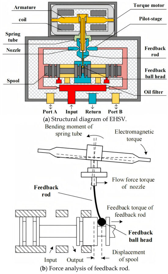
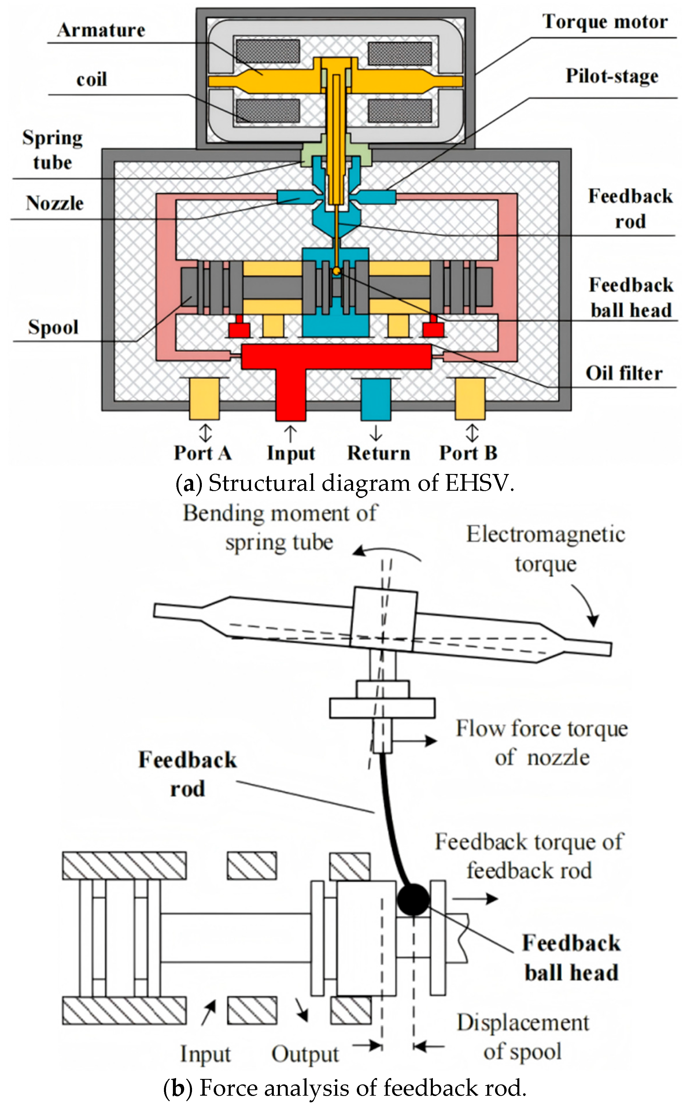
Electrohydraulic servo valves (EHSVs) are pivotal components in hydraulic servo-control systems, and their behavior governs both steady-state and dynamic performance. An EHSV transduces an electrical input into a spool displacement that is polarity-dependent, proportional, and precisely controlled. As shown in Figure 1a, adjusting the valve orifice regulates the flow rate and, in turn, the actuator motion. During spool reciprocation, the feedback ball head serves as the primary load-bearing element; as depicted in Figure 1b, it rolls within its mating ball socket.
Figure 1.
(a) Structure of the EHSV with the feedback rod at the neutral position; (b) Free-body diagram of the feedback-rod assembly under bending.
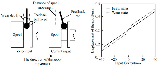
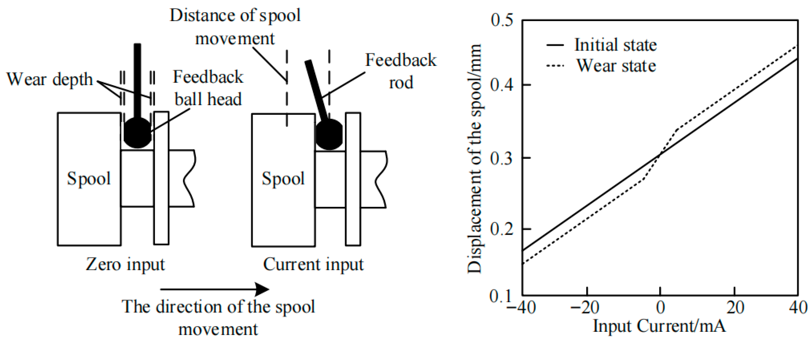
As shown in Figure 2, wear at the feedback ball head–ball seat interface changes the original contact geometry and introduces an additional clearance or wear depth . This wear-induced clearance weakens the mechanical feedback force transmitted from the spool to the armature-feedback assembly. As a result, the balance of the force feedback mechanism is disturbed, and a nonlinear region appears in the output characteristic. Therefore, the wear depth of the feedback ball head is selected as the key degradation variable in this study.
Figure 2.
Schematic illustrating the effects of feedback ball-head wear.
2.2. Fractal Representation of Rough Surfaces
Surface topography controls the number, height, and spatial distribution of asperities at a contact and, consequently, the interfacial wear rate. Robust description of this microstructure is therefore fundamental to constructing wear models. Traditional characterizations largely rely on statistical metrics and stochastic-process theory, but the resulting descriptors are often sensitive to sampling length and instrument resolution. At the microscopic scale, contact surfaces exhibit inherent features: disorder, randomness, fractality, multiscale structure, and self-affinity. In practice, the Weierstrass Mandelbrot (W-M) function from fractal geometry is widely used to represent rough surface microstructure.
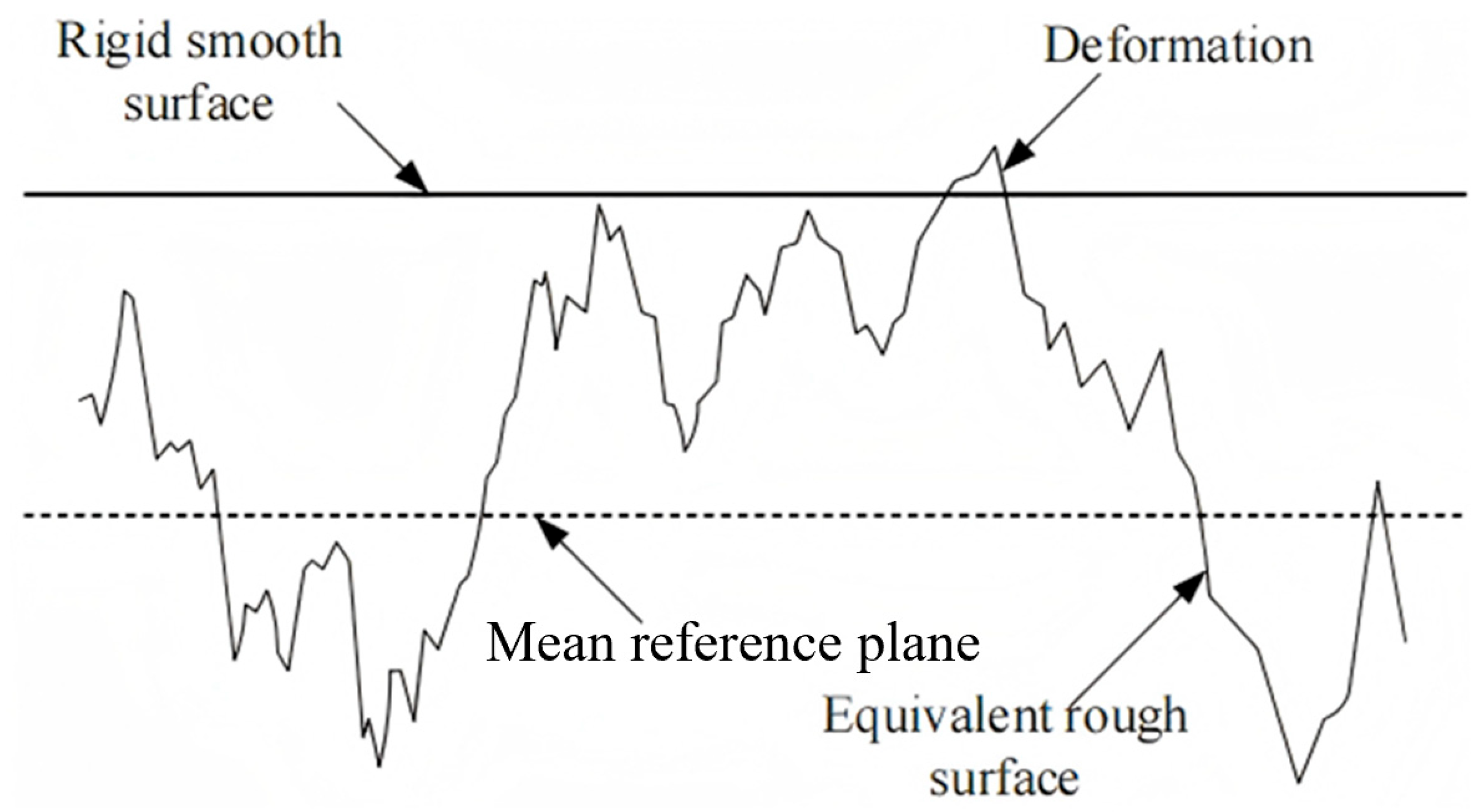
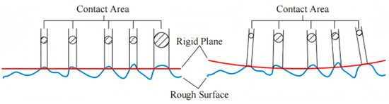
As illustrated in Figure 3, the contact of two rough bodies during wear can be idealized as an equivalent rough surface pressed against a rigid plane. In this schematic, the mean reference plane is introduced only as a geometric datum for defining the asperity height, summit position, and normal deformation in the fractal contact model. It should not be confused with roughness parameters such as the areal arithmetic mean height or the profile arithmetic mean roughness . The fractal-surface model is developed under three assumptions: (i) the equivalent surface is isotropic and exhibits fractal characteristics; (ii) asperity contacts act independently no asperity asperity interaction occurs and no volumetric deformation arises so under small global perturbations (light loading) the mean spacing between individual contacts is much larger than their characteristic size; and (iii) in the spectral description, only the maximum wavelength of the truncated profile is retained, meaning smaller bumps superposed on the dominant summit are neglected.
Figure 3.
Equivalent fractal rough-surface contact model.
Based on fractal surface theory and the W-M function widely used for rough-surface characterization [30,31,32], the isotropic two-dimensional rough profile can be simplified as follows:
where D and G are the fractal dimension and scaling coefficient, respectively. γn is the discrete frequency modes, n is the frequency index, and x the spatial coordinate.
The expression for the contour curve of a single asperity before deformation is
The peak height of the asperity before deformation is
The curvature radius of the top of asperity can be expressed as
Accordingly, the summit radius of curvature is not constant, its value varies with the real contact area a.
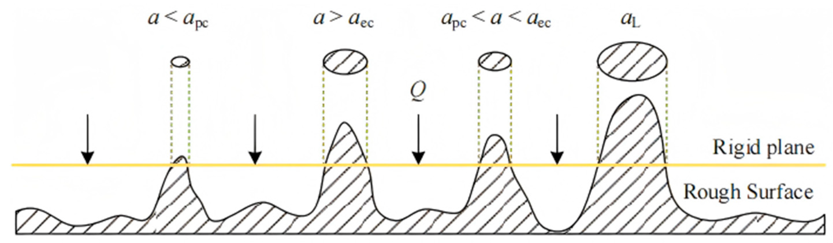
As illustrated in Figure 4, actual contact is intrinsically multiscale, involving simultaneous interactions among many asperity summits. Under a normal load Q, these summits experience different degrees of deformation. To more accurately represent this response and to compute the true contact area, a multiscale framework is adopted that partitions the deformation of an individual asperity into three regimes: elastic, elastoplastic, and fully plastic.
Figure 4.
Schematic diagram of multi-scale contact state.
2.3. Multiscale Contact Model
2.3.1. Elastic Deformation Stage
Based on Hertzian contact theory and fractal asperity contact models [33,34], the deformation of a single asperity is divided into elastic, elastoplastic, and plastic stages. In the elastic stage, the critical elastic deformation can be expressed as follows:
where Q denotes the normal load applied to the rough surface, and Eeq is the equivalent Young’s modulus.
For metallic materials, if Poisson’s ratio is assumed temperature-independent, thermal softening in the elastic-contact regime is represented via a temperature-dependent Young’s modulus. The modulus temperature relationship can then be written as
where E0 is the elastic modulus at temperature T0, α is the rate of change in the elastic modulus with temperature.
The flash point temperature rise in the contact point can be expressed as
where k is the friction coefficient of the contact surface, Q is the load applied per unit area, v is the relative velocity of motion, ω is the micro-motion frequency, τ is the thermal conductivity, c is the specific heat capacity.
The expression for the equivalent of Young’s modulus is
where µ1 and µ2 are the Poisson’s ratios of the materials at the two contact surfaces, and E1 and E2 are the Young’s moduli of the components, respectively.
When the asperity on the contact surface yields
where kµ is the friction coefficient of the contact surface.
Therefore, the deformation of the asperity can be written as
The thermal softening property also affects the yield limit of materials, and the yield limit of metal materials at temperature T is
when a > aec, it is in the stage of elastic deformation, and the critical elastic contact area can be written as
2.3.2. Elastic Plastic Contact Stage
The following equation determines the critical contact area between elasticity and plasticity
where r represents the radius of the contact point.
For strain-hardening materials, the following relationship exists
where m represents the strain hardening index.
The strain at the top of the asperity is expressed as
The expression between the top radius Rep and the contact area a is
When aec < a < apc, the critical plastic deformation is expressed as
where
2.3.3. Plastic Contact Stage
When a < apc, the contact point undergoes plastic deformation.
The top radius of the asperity during elastic plastic deformation is
Therefore, when the contact area a is smaller than the critical plastic transformation area apc, the deformation of the asperity δ > δec, and plastic deformation occurs at the contact point. When the contact area a is smaller than the critical elastic conversion area aec and larger than the plastic conversion area apc, the contact point undergoes elastic plastic deformation. When the contact area a is larger than the critical elastic conversion area apc, the deformation of the asperity δ < δec, and the contact point undergoes elastic deformation.
2.4. Fractal Wear Model Based on Archard Law
Archard’s wear law was adopted as the basic wear formulation because it provides a physically interpretable relationship among wear depth, normal load, sliding distance, hardness, and wear coefficient. In this study, other wear laws were not independently tested. However, the classical Archard model was modified by relating the wear coefficient and real contact area to the time-varying fractal parameters of the worn surface.
According to Archard’s classical wear law [15], the wear depth can be related to the real contact area, normal load, hardness, and relative sliding distance, and can be written as follows:
where Kabh is the wear coefficient, Ar is the actual contact area, Qc is the normal load, H is the hardness, and xb is the relative sliding distance.
In this work, the primary wear indicator is the wear depth , rather than the wear coefficient . The wear depth directly reflects the clearance change at the feedback ball head–ball seat interface and is closely related to the nonlinear output of the servo valve. In the Archard-based model, the wear volume is first calculated from the normal load, sliding distance, hardness, and wear coefficient, and then converted into wear depth according to the contact geometry. The wear coefficient is treated as a time-varying model parameter determined by the fractal characteristics of the worn surface.
The wear coefficient and the actual contact area are related to the surface morphology. As the wear process progresses, the surface morphology exhibits temporal variability. Therefore, this study establishes a mathematical model that relates these variables to the fractal parameters and . The servo-valve mechanical model is used to calculate the normal load and the relative sliding distance , both of which vary with the wear process.
2.4.1. Fractal Model of Wear Coefficient
Since the wear coefficient is affected by the friction state and asperity deformation, the relationship between the wear coefficient and friction coefficient is introduced based on asperity contact mechanics and the Tresca yield criterion as follows:
where kµ is the friction coefficient.
Based on the stress state of the microcontact boundary and the Tresca yield condition, the relationship between the normal load and the tangential load on the asperity is
When the tangential load on the asperity reaches its limit, all asperities in incomplete plasticity will be emitted. At this point, relative sliding occurs on the contact surface, and the tangential load is the maximum static friction force.
where the subscript np represents the non-plastic part.
The contact area A of the nonplastic part can be expressed as
The definition of the static friction coefficient on the contact surface is the ratio of the maximum tangential load to the normal load.
As the above formulas show, the friction coefficient of a material is related to its properties, contact area, and surface roughness. Combining the above formulas yields the wear coefficient Kabh.
2.4.2. Fractal Model of Real Contact Area
Based on simulating rough contours using the W-M function, it is necessary to introduce a density distribution function. For a given contact area a, the number of asperities larger than area a in the contact area can be obtained
where aL is the largest contact area.
The contact area distribution function of asperity can be written as
where represents the coefficient of expansion, expressed as
The above expression only applies to the contact between two rough planes and does not apply to cases where the plane is not a curved, cylindrical, or spherical surface. As shown in Figure 5, the surfaces of the ball and spool are spherical. Due to the different surface shapes, the actual contact state will also vary, so it needs to be corrected.
Figure 5.
Schematic diagram of contact between rough plane and rough surface.
Construct contact load coefficients for rough surfaces using fractal contact and Hertz elastic contact theories. Because the feedback ball head–ball seat interface is a spherical contact pair rather than a nominally flat rough contact, a geometric correction coefficient λ is introduced to modify the asperity contact-area distribution:
The expression for the surface contact coefficient λ is
where rb and rs are the curvature radii of the feedback rod ball and the ball hole on the spool, respectively.
The actual contact area between the feedback rod ball head and the ball hole can be expressed as
where aL is an unknown variable that needs to be solved. To calculate the actual contact area, it is necessary to calculate the load on all asperities at each deformation stage. The contact load on the contact surface is the sum of the contact loads at all contact points, and the load distribution on the entire contact surface is obtained through integration.
When a < apc, then
When apc < a < aec, then
When a > aec, then
where
The maximum contact area aL can be calculated by incremental iteration based on the force balance equation in the normal direction of the contact surface. On this basis, calculate the actual contact area using Equation (32).
2.5. Gaussian-Process-Based Prediction of Fractal Parameters
Studying the evolution law of fractal parameters can identify the running in state and describe the running process, which is of great significance for quantitative research on wear problems. Since the evolution of the fractal parameters is independent of the initial parameters, considering stiffness degradation and the increase in wear of the feedback rod that connects the ball head, this paper uses machine learning methods to describe the evolution of the fractal parameters. Gaussian process regression [35] is suitable for handling small-sample and nonlinear regression problems and has strong generalization ability.
This section uses the fractal parameters of each node in the numerical simulation as the data set. Based on Gaussian process regression, establish fractal parameter predictions corresponding to different displacements and cycle times.
where ω represents the fractal parameter obtained by fitting the Gaussian process regression, z = [xv, t]T, xv and t represent the displacement of the spool and the number of cycles, respectively. m(z) and k(z, z′) are the mean and kernel functions of Gaussian processes, respectively. By comparing the RMSE of the fitting results, Matérn 5/2 was chosen as the kernel function used in this article. The data set is divided into subsets to verify whether the model is overfitting. Select one subset as the validation set and the remaining subsets as the training set to train the model. During the model training process, all data are normalized to improve the accuracy and convergence speed of the model.
The response surfaces of the fractal parameters were generated using Gaussian process regression based on the experimentally identified fractal parameters. The input variables were the loading displacement and the number of loading cycles , while the output variables were the fractal dimension and characteristic scale of the ball head and ball seat. After data normalization, a Matérn 5/2 kernel was used to fit the nonlinear mapping between the operating conditions and the fractal parameters. The trained model was then used to generate response surfaces over the displacement-cycle domain.
Based on this data set, given the prior mean functions m(z) = 0 and k(z, z′), a posterior estimate of the test point z can be obtained.
where K is the Gram matrix.
2.6. Servo-Valve Mechanical Model and Wear-Depth Calculation
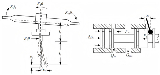
Figure 6 is a schematic diagram of the motion of the armature feedback rod assembly. The torque balance equation of the armature feedback rod assembly is
where Kt is the median electromagnetic torque coefficient of the torque motor, ic is the input current, Km is the median electromagnetic spring stiffness of the torque motor, and θ is the rotation angle of the armature. Ka is the stiffness of the spring tube, Kf is the flow force stiffness, Fb is the feedback force of the feedback rod, la is the distance from the axis of the pilot stage jet to the center of rotation of the armature, and lb is the distance from the center of the ball of the feedback rod to the axis of the jet.
Figure 6.
Schematic diagram of the motion of the feedback rod assembly.
The elasticity of the armature and nozzle has little effect on the displacement of the feedback rod, and are considered rigid bodies in this article. The contact load between the ball and the ball hole at the contact interface consists of two parts, one is the force generated by the input control current causing the armature feedback rod assembly to deflect, and the other is the force generated by the pressure difference in the control chamber pushing the valve core to move. If the feedback rod ball is unconstrained, its displacement is mainly caused by the deformation of the baffle and spring tube. When the ball moves in the ball hole, the displacement of the valve core imposes displacement constraints on the ball head. The normal contact load on the ball can be described as
where xb is the axial displacement of the ball head, ωH is the wear depth. The calculated contact load is compared with the normal load, and the maximum contact area aL is obtained by the Newton Raphson method.
The relative sliding distance between the ball head and the ball hole can be calculated through the displacement of the spool.
The normal contact load in Equation (43) is obtained from the displacement constraint between the ball head and the ball seat, while the relative sliding distance in Equation (44) is calculated from the spool displacement and the geometric relationship of the feedback mechanism.
2.7. Algorithm Workflow of the Proposed Wear-Prediction Framework
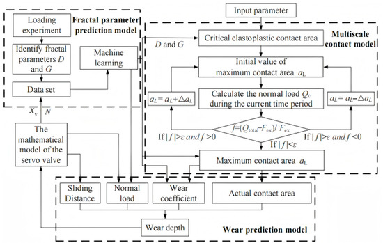
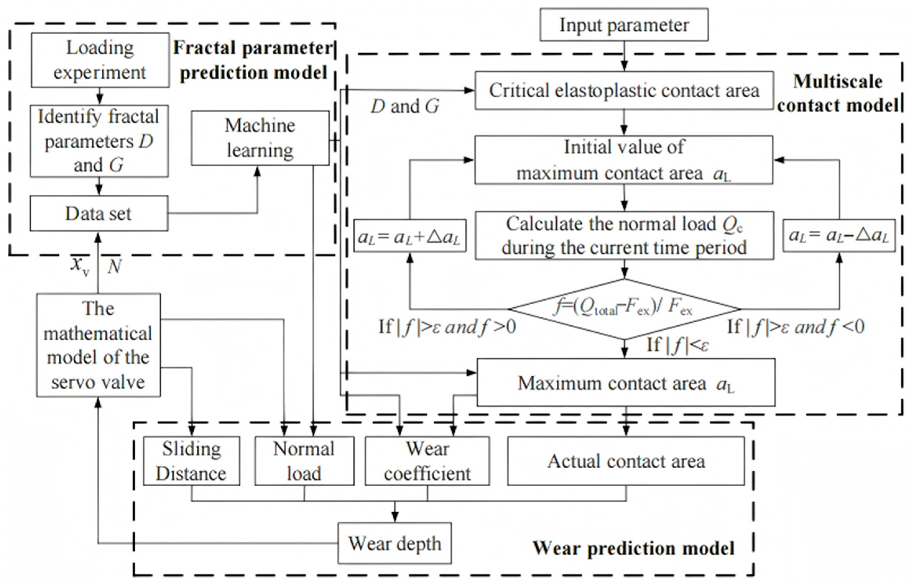
To clarify the implementation procedure of the proposed model, the complete wear-prediction workflow is summarized in Figure 7.
Figure 7.
Flowchart of the proposed wear-prediction framework.
As shown in Figure 7, the proposed framework includes parameter initialization, fractal-parameter prediction, multiscale contact calculation, wear-depth prediction, model updating, and experimental validation. The detailed procedure is as follows:
- Parameter initialization. The structural parameters, material parameters, loading conditions, and initial surface morphology parameters of the feedback ball head–ball seat interface are initialized.
- Fractal-parameter prediction. Worn-surface profiles are obtained from repeated loading experiments, and the fractal parameters are identified using the structural-function method. A Gaussian process regression model is then trained using the loading cycles and displacement loads as inputs and the fractal parameters as outputs.
- Multiscale contact calculation. The predicted fractal parameters are introduced into the multiscale contact model to determine the contact state of asperities, including elastic, elastoplastic, and plastic deformation stages. The critical contact areas and the real contact area are then calculated.
- Wear-depth prediction and model updating. The Archard-based fractal wear model is used to calculate the wear depth. In this process, the servo-valve mechanical model provides the normal contact load and relative sliding distance, while the wear coefficient and real contact area are updated according to the predicted fractal parameters. The calculated wear state is then fed back to update the contact geometry and model parameters for the next loading step.
- Experimental validation. The predicted fractal parameters and wear depth are compared with experimental results obtained from repeated loading tests and white-light interferometry measurements to evaluate the accuracy of the proposed method.
3. Results and Discussion
3.1. Experimental Setup and Surface-Profile Measurement
The repeated loading tests were conducted under a room-temperature laboratory environment, and no additional thermal loading or controlled humidity treatment was applied during the tests. Pre-test data were used to construct the training set for the fractal-parameter predictor, whereas validation tests evaluated the wear-prediction algorithm. In the pretests, the controlled variables were the number of loading cycles N and the applied load Q. The load Q equals the ball-head force Fb and is computed from Equation (43). Accordingly, Q was prescribed via the screw-module travel xv, which was set by the number of pulses delivered to the servo motor. Six displacement amplitudes were used: 0.40, 0.41, 0.42, 0.43, 0.44, and 0.45 mm. The loading process was governed by the pulse frequency of the servo motor, which was set to 200 kHz. For each displacement amplitude, surface profiles were acquired at N = 0, 2000, 4000, 6000, 8000, 10,000, 12,000, 14,000, and 16,000 cycles. Thus, the experimental duration for each loading condition was defined by the cumulative number of loading cycles, and the wear evolution was monitored until 16,000 cycles.
It should be noted that the measurements were time-series repeated-loading measurements for each loading condition, rather than independent repeated tests using multiple specimens for every condition. This experimental design was adopted because the purpose of the test was to capture the progressive evolution of surface morphology and wear depth during repeated sliding.
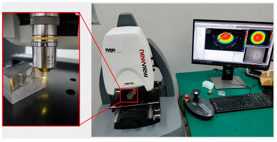
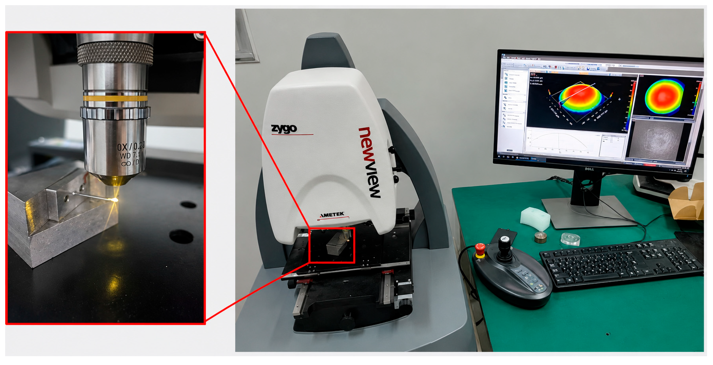
Surface topography and contour profiles were characterized using a white-light interferometer (WLI), as shown in Figure 8. The WLI was used to measure the worn surfaces of the feedback ball head and its mating ball seat/groove and to obtain both two-dimensional contour profiles and three-dimensional surface reconstructions. The vertical resolution of the instrument was less than 0.08 nm, the lateral sampling range was 0.34–16.42 μm, and the RMS repeatability was less than 0.008 nm. For each measured surface, the contour curve along the central axis of the contact region was extracted and used for structural-function-based fractal parameter identification. Since the wear depth at the feedback ball head–ball seat interface is very small, non-contact optical profiling was used to capture the surface contour evolution without damaging the worn surfaces. This approach is suitable for identifying small surface-morphology changes and evaluating wear-depth evolution in precision contact pairs [36,37].
Figure 8.
White-light interferometry setup for surface-profile measurement.
3.2. Fractal-Parameter Identification and Evolution
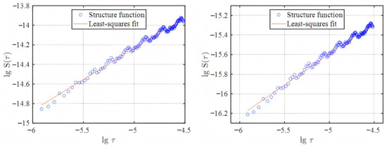
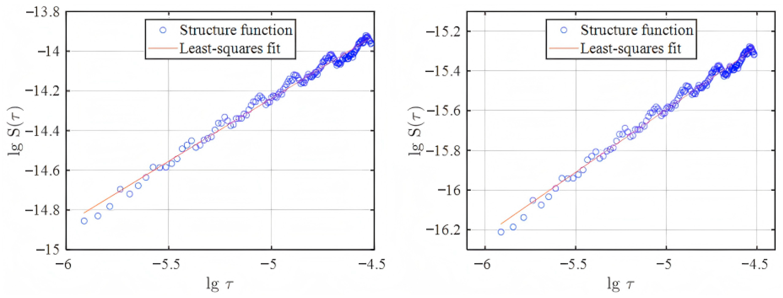
Before the repeated loading tests, the initial surface profiles of the feedback ball head and ball seat were measured and analyzed using the structural-function method. Figure 9 shows the structural-function fitting results of the initial contour curves. The approximately linear relationship in the log–log coordinate system indicates that the measured profiles exhibit fractal characteristics within the selected scale range. Linear least-squares fitting gave correlation coefficients of 0.927 for the ball head and 0.972 for the ball seat, indicating acceptable fitting quality. The initial fractal parameters were identified as , m for the ball head and , m for the ball seat. These parameters were used as initial inputs for the subsequent
contact and wear calculations.
Figure 9.
Structural function of surface contour curves of ball head and ball hole.
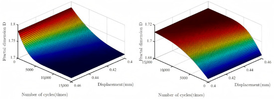
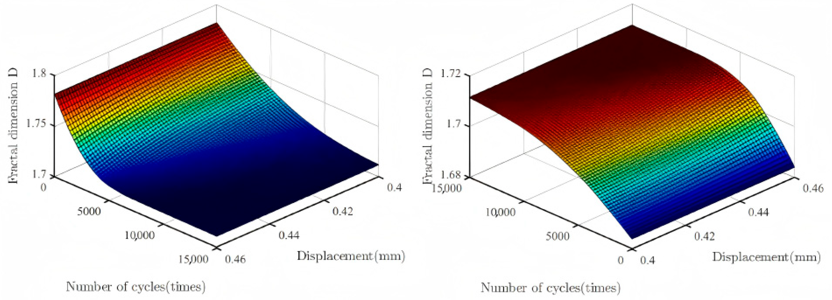
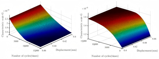
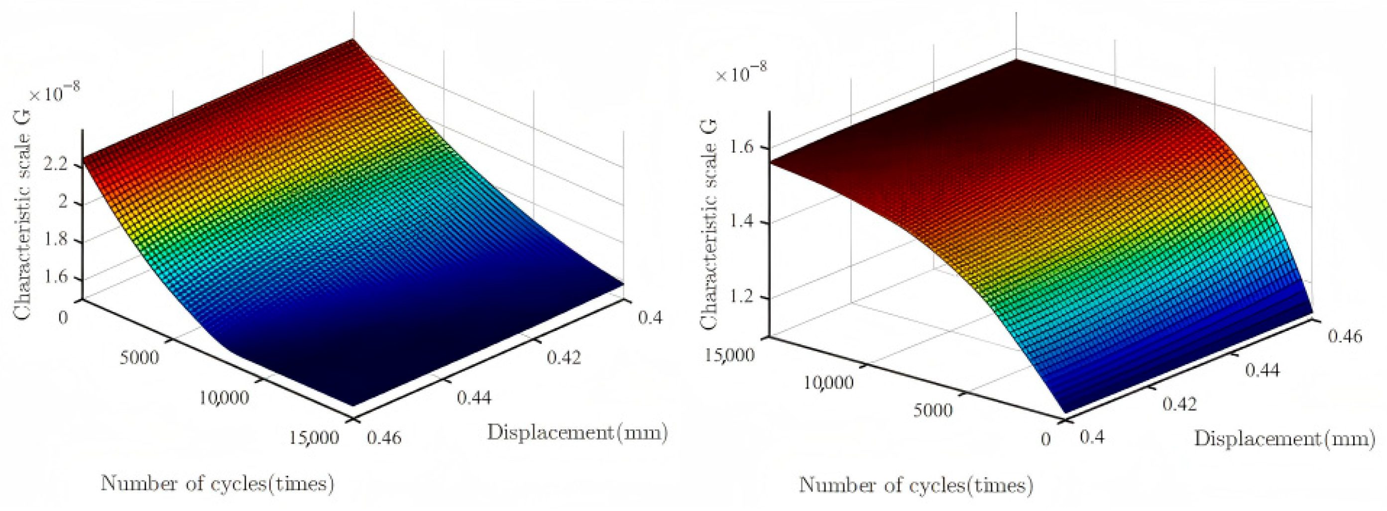
Based on the Gaussian-process-based response-surface generation method described in Section 2.3, the fitted response surfaces of the fractal dimension , and characteristic scale under different loading displacements and cycle numbers are shown in Figure 10 and Figure 11, respectively. The surface morphology of the friction pair during wear exhibits significant fractal characteristics, which can be characterized by scale-independent fractal parameters. Surface features can have an impact on the wear process and wear can also alter the surface morphology. To obtain the evolution law of the fractal dimension and characteristic scale during the wear process, we collected the surface morphology of the ball head and ball hole at different collection points using a white light interferometer. Extract the contour curve on the central axis and calculate the fractal dimension and characteristic scale of the contour curve using the structural function method. The fractal dimension reflects the complexity of the surface contour, while the characteristic scale is related to the amplitude of surface asperities. During wear, the two parameters change simultaneously, indicating the continuous evolution of surface morphology. The characteristic scale corresponds to a decrease in the amplitude of the contour curve, that is, a decrease in surface roughness, which means that the surface becomes smoother and smoother.
Figure 10.
Fitting surface of fractal dimension.
Figure 11.
Fitting surface of characteristic scale.
The fractal parameters change more obviously during the running-in stage than during the later stable-wear stage. This is mainly because high asperities on the initially rough surface are preferentially removed or plastically deformed during repeated sliding contact. As wear progresses, the contact surfaces gradually become more compatible, and the variation rate of the fractal parameters decreases.
It should be noted that the evolution of fractal dimension is affected by the initial surface state of each mating component. Therefore, the ball head and ball seat may show different local trends, rather than a strictly monotonic change in every curve. For the initially rougher ball seat, the removal of high asperities tends to smooth the surface, while the relatively smoother ball head may become slightly rougher due to micro-ploughing, adhesion, or material transfer during contact. Therefore, the main feature of the running-in process should be understood as the gradual convergence of the fractal parameters of the two mating surfaces.
When the number of cycles reaches a certain level, the fractal dimension and characteristic scale tend to stabilize, indicating that the contact pair gradually enters the stable-wear stage. Differences in loading displacement may lead to differences in the number of cycles required to complete the running-in process. Once the stable-wear stage is reached, the ball head and ball seat maintain relatively close fractal parameters, indicating the formation of a more stable and mutually compatible contact state.
3.3. Model Validation and Wear-Depth Prediction
To ensure the reliability of the proposed prediction method, the model was validated from three aspects. First, the fractal-parameter prediction model was trained using pretest data under different displacement loads and loading cycles, and validation subsets were used to check the generalization ability of the Gaussian process regression model. Second, an independent variable-amplitude loading test was conducted to evaluate the prediction performance under time-varying loading conditions. Third, the predicted fractal parameters and wear depths were compared with experimental measurements obtained by white-light interferometry and structural-function analysis.
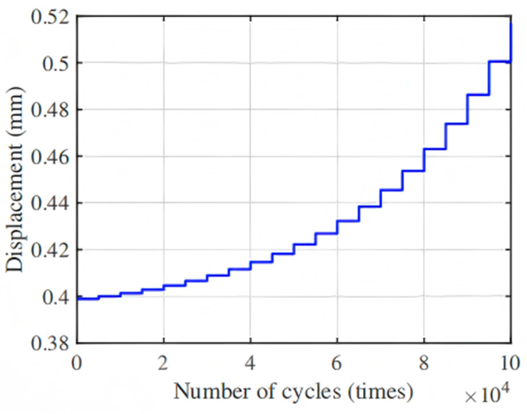
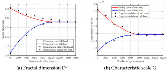
Therefore, verification experiments were conducted using the time-varying load spectrum shown in Figure 12. The fractal dimension and characteristic scale of the collected contour curves were calculated using the structural-function method, and the comparison results between the fractal parameters obtained from the verification experiment and the Gaussian process regression fitting curve are shown in Figure 13.
Figure 12.
Load spectrum.
Figure 13.
Simulation curves and experimental data of fractal parameters.
The results show that the fractal dimension and characteristic scale evolution characteristics of the experimental results are close to the simulation results. After the start of wear, it changes rapidly at a large rate, and the rate of change gradually decreases as the wear progresses. Among them, the dimension of the rougher ball hole increased from the initial 1.684 to 1.7516, while the fractal dimension of the relatively smooth ball head decreased from 1.7818 to 1.7514. The characteristic scales show a similar trend of change, with the characteristic scales of the ball head and ball hole varying from 2.25 × 10⁻⁸ m and 1.12 × 10⁻⁸ m, respectively, to around 1.57 × 10⁻⁸ m. After reaching 12,000 cycles, the fractal parameters tend to stabilize. The error between the experimental and predicted fractal parameters does not exceed 3%, indicating that the Gaussian process regression model can effectively capture the evolution of surface morphology under variable-amplitude loading conditions.
To evaluate the deviation between experimental and simulated results, the predicted fractal parameters and wear depths were compared with the values obtained from white-light-interferometry profiles and structural-function analysis. The prediction error of the Gaussian process regression model for the fractal parameters was below 3%. For wear-depth prediction, the deviation between the simulated and measured results remained within approximately 1%, indicating that the proposed model can describe the time-varying wear behavior of the feedback ball head-ball seat interface with acceptable accuracy.
For the relatively rough ball-seat surface, the initial wear rate was relatively high and then decreased rapidly from 7.28 × 10⁻⁹ m/cycle. After approximately 12,000 cycles, it stabilized around 1.11 × 10⁻⁹ m/cycle. For the relatively smooth ball-head surface, the wear rate was initially lower and gradually increased from 3.45 × 10⁻¹⁰ m/cycle to approximately 1.11 × 10⁻⁹ m/cycle, after which it remained relatively stable during subsequent cyclic loading. These results indicate that the proposed method can capture both the rapid morphology evolution during the running-in stage and the stable wear behavior after the contact pair becomes more compatible.
Compared with classical Archard-type wear models [15], the proposed method updates the wear coefficient and real contact area according to the predicted fractal parameters, rather than treating them as constants. Existing fractal contact models have shown that surface morphology affects asperity deformation and real contact area [30,31,32,33,34], while previous studies on hydraulic and servo-valve wear mainly focused on spool–sleeve wear, abrasive wear, or performance degradation [25,26,27,28,29]. In contrast, this study focuses on the feedback ball head–ball seat interface and couples fractal-parameter evolution with the servo-valve mechanical model. This allows the proposed framework to describe the transition from running-in wear to stable wear and to provide a more physically interpretable wear-depth prediction.
4. Conclusions
In this study, a wear-prediction framework combining fractal contact theory, Archard wear law, Gaussian process regression, and a servo-valve mechanical model was proposed for the feedback ball head–ball seat interface. The main conclusions are as follows:
The proposed model updates the real contact area and wear coefficient according to time-varying fractal parameters, rather than treating them as constants. This improves the physical interpretability of wear-depth prediction during repeated sliding contact.
During the running-in stage, the fractal dimension of the ball seat increased by approximately 4.01%, while that of the ball head decreased by approximately 1.71%. The characteristic scales of the two contact surfaces gradually converged to approximately 1.57 × 10⁻⁸ m.
After approximately 12,000 cycles, the fractal parameters tended to stabilize, indicating that the contact pair gradually entered a stable wear stage. This result shows that the proposed method can capture the transition from running-in wear to stable wear.
The prediction error of the Gaussian process regression model was below 3%, and the wear-depth prediction error remained within approximately 1%. These results verify the effectiveness of the proposed wear-prediction framework for describing the time-varying wear evolution of the feedback ball head–ball seat interface.
Author Contributions
Conceptualization, X.P.; software, J.Z.; validation, J.K.; writing—original draft preparation, X.P. All the data used in the simulation analysis in this paper are available. All authors have read and agreed to the published version of the manuscript.
Funding
This research was supported in part by the Innovation Fund Project for University Teachers in Gansu Province (2025B-215), the Key Research and Development Program of Gansu Province–Industrial Project (25YFGM002), the Qingyang City Major Science and Technology Project–Industrial Field Project (2025JY1005), the Longdong University Higher Education Teaching Research 2026 Key Project (LYJYJX2026A45), the Longdong University Horizontal Research Project (HXZK2547), Scientific Research Projects of Higher Education Institutions in Gansu Province (2026QB-096), and the Natural Science Foundation of Gansu Provincial Department of Science and Technology (24JRRM004).
Data Availability Statement
The original contributions presented in this study are included in this article. Further inquiries can be directed to the corresponding author.
Acknowledgments
The authors would like to thank the Robot Laboratory of the School of Intelligent Manufacturing, Longdong University, for providing the experimental equipment and workspace. This research was made possible through collaborative efforts and technical support from the robotics research team.
Conflicts of Interest
The authors declare no conflicts of interest.
Nomenclature
| D | Fractal dimension | – |
| G | Characteristic scale coefficient | m |
| a | Contact area of a single asperity | m2 |
| aL | Maximum contact area | m2 |
| aec | Critical elastic contact area | m2 |
| apc | Critical plastic contact area | m2 |
| Ar | Real contact area | m2 |
| Qc | Normal contact load | N |
| H | Hardness | Pa |
| xb | Relative sliding distance | m |
| wH | Wear depth | m |
| Kabh | Wear coefficient | – |
| kµ | Friction coefficient | – |
| Eeq | Equivalent Young’s modulus | Pa |
| E1, E2 | Young’s moduli of the two contact materials | Pa |
| µ1, µ2 | Poisson’s ratios of the two contact materials | – |
| N | Number of loading cycles | – |
| xv | Loading displacement/spool displacement | m |
| Fb | Feedback force of the feedback rod | N |
| mz | Mean function of Gaussian process regression | – |
| k(z,z’) | Kernel function of Gaussian process regression | – |
References
- Sharma, A.K.; Kumar, N.; Das, A.K. A review on wear failure of hydraulic components: Existing problems and possible solutions. Eng. Res. Express 2024, 6, 012502. [Google Scholar] [CrossRef] [Scilit]
- Yang, Y.J.; Peng, W.; Meng, D.; Zhu, S.P.; Huang, H.Z. Reliability analysis of direct drive electrohydraulic servo valves based on a wear degradation process and individual differences. Proc. Inst. Mech. Eng. Part O J. Risk Reliab. 2014, 228, 621–630. [Google Scholar] [CrossRef] [Scilit]
- Ren, J.; Zhao, B.; Quan, L.; Lan, Y.; Li, Y.; Hao, Y. Research on proportional valve spool wear diagnostic method hybrid-driven by the valve port energy loss mechanism model and data. Mech. Syst. Signal Process. 2024, 219, 111606. [Google Scholar] [CrossRef] [Scilit]
- Liao, Y.; Tao, Z.; Lian, Z. Design, failure analysis, and optimization of a high-flow water valve: A case study. Proc. Inst. Mech. Eng. Part E J. Process Mech. Eng. 2023, 237, 1331–1343. [Google Scholar] [CrossRef] [Scilit]
- Stachowiak, G.W.; Batchelor, A.W. Engineering Tribology, 4th ed.; Butterworth-Heinemann: Oxford, UK, 2014. [Google Scholar]
- Bhushan, B. Introduction to Tribology, 2nd ed.; John Wiley & Sons: Hoboken, NJ, USA, 2013. [Google Scholar]
- Xie, W.; Jiang, D.; Jin, J.; Liu, C. Single-asperity failure mechanism driven by morphology and multiaxial loading using molecular dynamics simulation. Comput. Mater. Sci. 2022, 213, 111671. [Google Scholar] [CrossRef] [Scilit]
- Carvalho, R.P.; Carneiro, A.M.C.; Pires, F.M.A.; Doca, T. An efficient multiscale strategy to predict the evolution of the real contact area between rough surfaces. Tribol. Int. 2022, 165, 107255. [Google Scholar] [CrossRef] [Scilit]
- Mu, X.; Sun, Q.; Xu, J.; Chai, Z.; Sun, W.; Zhao, B. Feasibility analysis of the replacement of the actual machining surface by a 3D numerical simulation rough surface. Int. J. Mech. Sci. 2019, 150, 135–144. [Google Scholar] [CrossRef] [Scilit]
- Kogut, L.; Etsion, I. Elastic-plastic contact analysis of a sphere and a rigid flat. J. Appl. Mech. 2002, 69, 657–662. [Google Scholar] [CrossRef] [Scilit]
- Ge, S.; Tonder, K. The fractal behavior and fractal characterization of rough surfaces. Tribology 1997, 17, 73–80. [Google Scholar]
- Wei, L.; Liu, Q.; Zhang, P. Sliding friction surface contact mechanics model based on fractal theory. J. Mech. Eng. 2012, 48, 106–113. [Google Scholar] [CrossRef]
- Wang, G.; Wang, L.; Yuan, Y. Investigation on dynamics performance of multibody system with rough surface. Appl. Math. Model. 2022, 104, 358–372. [Google Scholar] [CrossRef] [Scilit]
- Gordillo, O.; Hincapie, W.; Piamba, O.; Olaya, J.; Trava-Airoldi, V. Study of adhesive wear test on TiSi, AlTi, and WTi coatings. Coatings 2022, 12, 1370. [Google Scholar] [CrossRef] [Scilit]
- Archard, J.F. Contact and rubbing of flat surfaces. J. Appl. Phys. 1953, 24, 981–988. [Google Scholar] [CrossRef] [Scilit]
- Hutchings, I.M.; Shipway, P. Tribology: Friction and Wear of Engineering Materials, 2nd ed.; Butterworth-Heinemann: Oxford, UK, 2017. [Google Scholar]
- Greenwood, J.A.; Williamson, J.B.P. Contact of nominally flat surfaces. Proc. R. Soc. Lond. A 1966, 295, 300–319. [Google Scholar] [CrossRef] [Scilit]
- Whitehouse, D.J.; Archard, J.F. The properties of random surfaces of significance in their contact. Proc. R. Soc. Lond. A 1970, 316, 97–121. [Google Scholar] [CrossRef] [Scilit]
- Onions, R.A.; Archard, J.F. The contact of surfaces having a random structure. J. Phys. D Appl. Phys. 1973, 6, 289–304. [Google Scholar] [CrossRef] [Scilit]
- Nayak, P.R. Random process model of rough surfaces in plastic contact. Wear 1973, 26, 305–333. [Google Scholar] [CrossRef] [Scilit]
- Thomas, T.R. Surface topography in tribology. Phys. Bull. 1982, 33, 326–328. [Google Scholar] [CrossRef] [Scilit]
- Majumdar, A.; Tien, C.L. Fractal characterization and simulation of rough surfaces. Wear 1990, 136, 313–327. [Google Scholar] [CrossRef] [Scilit]
- Majumdar, A.; Bhushan, B. Fractal model of elastic-plastic contact between rough surfaces. J. Tribol. 1991, 113, 1–11. [Google Scholar] [CrossRef] [Scilit]
- Wang, S.; Komvopoulos, K. A fractal theory of the interfacial temperature distribution in the slow sliding regime: Part II—Multiple domains, elastoplastic contacts and applications. J. Tribol. 1994, 116, 824–832. [Google Scholar] [CrossRef] [Scilit]
- Gong, W.; Chen, Y.; Li, M.; Kang, R. Coupling fractal model for adhesive and three-body abrasive wear of AISI 1045 carbon steel spool valves. Wear 2019, 418–419, 75–85. [Google Scholar] [CrossRef] [Scilit]
- Chen, Y.; Gong, W.; Kang, R. Coupling behavior between adhesive and abrasive wear mechanism of aero-hydraulic spool valves. Chin. J. Aeronaut. 2016, 29, 1119–1131. [Google Scholar] [CrossRef] [Scilit]
- Liu, X.; Liu, F.; Ji, H.; Li, N.; Wang, C.; Lin, G. Particle erosion transient process visualization and influencing factors of the hydraulic servo spool valve orifice. Flow Meas. Instrum. 2023, 89, 102273. [Google Scholar] [CrossRef] [Scilit]
- Wang, X.H.; Li, Q.X.; Feng, Y.L. Research of double nozzle flapper valve accelerated degradation test. Appl. Mech. Mater. 2014, 532, 18–21. [Google Scholar] [CrossRef] [Scilit]
- Mi, J.; Huang, G. Dynamic prediction of performance degradation characteristics of direct-drive electro-hydraulic servo valves. Appl. Sci. 2023, 13, 7231. [Google Scholar] [CrossRef] [Scilit]
- Shen, F.; Li, Y.H.; Ke, L.L. A novel fractal contact model based on size distribution law. Int. J. Mech. Sci. 2023, 249, 108255. [Google Scholar] [CrossRef] [Scilit]
- Yuan, Y.; Xu, K.; Zhao, K. A fractal model of contact between rough surfaces for a complete loading-unloading process. Proc. Inst. Mech. Eng. Part C J. Mech. Eng. Sci. 2020, 234, 2923–2935. [Google Scholar] [CrossRef] [Scilit]
- Huang, G.; Liu, C.; Xie, W.; Jiang, D. Normal contact stiffness model for fractal surfaces considering scale dependence and friction behavior. Proc. Inst. Mech. Eng. Part J J. Eng. Tribol. 2023, 237, 527–540. [Google Scholar] [CrossRef] [Scilit]
- Johnson, K.L. Contact Mechanics; Cambridge University Press: Cambridge, UK, 1985. [Google Scholar] [CrossRef] [Scilit]
- Chen, J.; Liu, D.; Wang, C.; Zhang, W.; Zhu, L. A fractal contact model of rough surfaces considering detailed multi-scale effects. Tribol. Int. 2022, 176, 107920. [Google Scholar] [CrossRef] [Scilit]
- Rasmussen, C.E.; Williams, C.K.I. Gaussian Processes for Machine Learning; MIT Press: Cambridge, MA, USA, 2006. [Google Scholar]
- Leach, R. (Ed.) Optical Measurement of Surface Topography; Springer: Berlin/Heidelberg, Germany, 2011. [Google Scholar] [CrossRef] [Scilit]
- Jaturunruangsri, S. Evaluation of Material Surface Profiling Methods: Contact Versus Non-Contact. Master’s Thesis, Brunel University London, London, UK, 2015. [Google Scholar]
Disclaimer/Publisher’s Note: The statements, opinions and data contained in all publications are solely those of the individual author(s) and contributor(s) and not of MDPI and/or the editor(s). MDPI and/or the editor(s) disclaim responsibility for any injury to people or property resulting from any ideas, methods, instructions or products referred to in the content. |
© 2026 by the authors. Licensee MDPI, Basel, Switzerland. This article is an open access article distributed under the terms and conditions of the Creative Commons Attribution (CC BY) license.