Unsupervised Segmentation of Wear Surface Defects in Hydroturbine Bearing Pads Guided by Local Anomaly Scores

Abstract

Vision-based defect detection on bearing-pad wear surfaces is essential for quantifying damage geometry and assessing condition in hydroturbine units. Compared with 2D color images, depth images can suppress disturbances caused by complex textures, surface color variations, and specular reflections, thereby providing a more reliable basis for precise damage localization. Nevertheless, depth-based damage segmentation under a large field of view remains challenging, mainly due to fine-scale texture noise and weak defect saliency; moreover, robust defect probability estimation is often hindered by limited labeled data. To address these challenges, this paper proposes an unsupervised defect segmentation framework for hydroturbine friction components guided by local anomaly score distributions. First, a salient damage detection module is developed based on topography–texture separation, which mitigates the interference of local micro-texture noise on defect segmentation. Then, a normal reference dataset is constructed using defect-free bearing-pad depth images, and an unsupervised network is employed as the core to generate anomaly score representations of potential damage regions for coarse localization. Finally, the obtained anomaly score distribution is used as adaptive weights to fuse depth-based defect cues with morphological processing, enabling self-adaptive refinement of the damage regions. Experiments on real depth images acquired from hydroturbine bearing pads demonstrate that the proposed method achieves accurate defect extraction and reliable geometric quantification. Quantitative evaluations on the testing set yield a mean surface area error of 9.39% ± 4.25% and a volume error of 4.91% ± 2.85%, with best-case errors dropping as low as 3.67% and 1.03%, respectively. Crucially, these results demonstrate that our framework goes beyond mere visual detection; by operating entirely without pixel-level annotations, it offers a highly practical tool for diagnosing specific lubrication failure modes and driving predictive maintenance in actual hydroturbine engineering.

1. Introduction

The surface damage state of hydroturbine bearing pads is a critical indicator for evaluating operational safety and identifying potential failure mechanisms in hydropower units [1,2]. Accurate detection and localization of damage regions, along with quantitative characterization of their severity, are essential for condition monitoring, fault diagnosis, and predictive maintenance of hydroturbine systems. In practical engineering scenarios, bearing-pad damage such as wear, scuffing, pitting, and local spalling often evolves gradually under complex lubrication and load conditions. Particularly under severe operating loads, the hydrodynamic oil film is prone to localized thinning or catastrophic rupture, inevitably forcing the contact interface into a mixed lubrication regime. Once in this state, mechanical stress coupled with localized thermal activation rapidly accelerates the transition from mild wear to severe adhesive or abrasive damage [3]. Consequently, capturing and precisely quantifying the geometric footprint of these surface morphologies becomes the key to inversely diagnosing the underlying lubrication failure modes.

Vision-based surface damage analysis has been increasingly adopted as an effective non-contact approach for bearing-pad inspection, owing to its ability to capture geometric and morphological information of damaged surfaces [4,5]. Compared with conventional two-dimensional color images, depth images obtained from structured-light or 3D-scanning systems can effectively suppress disturbances caused by surface color variations, illumination changes, and specular reflections, thereby providing a more reliable basis for damage detection and geometric quantification [6,7]. However, damage detection in large-field-of-view depth imaging remains challenging, especially in the presence of fine-scale texture noise, gradual depth transitions, and blurred damage boundaries on worn bearing-pad surfaces.

Early vision-based damage detection methods for bearing pads and similar mechanical components primarily relied on manually designed geometric or texture features combined with traditional machine learning classifiers [8,9]. Although these approaches can achieve acceptable performance under controlled conditions, their effectiveness is highly dependent on expert knowledge and task-specific parameter tuning, resulting in limited generalization ability and high development costs [9,10]. To overcome these limitations, deep learning (DL)-based methods with automatic feature extraction have been widely adopted for surface damage detection and wear analysis [11].

Supervised DL models have initially dominated research on bearing surface damage detection by learning discriminative features from labeled damage images [12,13]. By annotating damage regions or types and feeding the labeled data into convolutional neural networks (CNNs), these methods can automatically localize and classify surface defects. For instance, region-based CNN architectures have been employed to identify damage locations and distinguish different wear mechanisms on mechanical components [14]. At the same time, pixel-level segmentation networks such as Mask R-CNN have been adopted for accurate extraction of wear regions from microscopic or macroscopic surface images [15]. Moreover, hybrid or multi-branch network structures have been proposed to assess damage morphology and severity [16] jointly.

Despite their effectiveness, supervised DL-based approaches suffer from several inherent limitations when applied to hydroturbine bearing-pad inspection. First, acquiring large-scale, high-quality labeled damage datasets is often impractical in industrial environments due to data scarcity, privacy concerns, and the high cost of expert annotation [17]. Second, the diversity and uncertainty of bearing-pad damage mechanisms can result in damage patterns of unknown morphology, which are difficult to predefine and label accurately. In addition, bearing-pad surfaces often exhibit numerous small-scale or blurred damage regions with multiple coexisting mechanisms, further increasing annotation complexity and reducing labeling reliability [18]. These issues significantly restrict the applicability of supervised learning paradigms in real-world hydropower maintenance scenarios.

To alleviate the dependence on extensive labeled data, unsupervised anomaly detection methods have recently emerged as a promising alternative for surface damage inspection [19]. These methods focus on modeling normal surface characteristics and identifying damage regions as anomalies that deviate from the learned normal patterns. Depending on the comparison strategy, existing unsupervised approaches can be broadly classified into image-similarity-based and feature-similarity-based methods. Image-level comparison approaches are intuitive and interpretable but are highly sensitive to noise and local misalignment at the pixel level [20]. In contrast, feature-based methods employ CNNs to extract high-dimensional representations and construct normal feature templates in the latent space, offering improved robustness against noise and local geometric variations [21,22,23].

Although unsupervised anomaly detection has demonstrated encouraging performance in surface damage detection, most existing methods still rely on pre-collected normal or unworn surface datasets as reference templates [24]. This requirement limits their applicability in scenarios where unworn bearing-pad data are unavailable or where surfaces exhibit time-varying wear evolution. Moreover, regions with uniform wear and anomalous damage often share similar feature representations, making it difficult to distinguish localized damage from global wear using conventional unsupervised models. Therefore, developing a completely unsupervised damage detection framework that does not depend on pixel-level defect annotations is of great significance for hydroturbine bearing-pad inspection.

In this study, a local anomaly score distribution-guided unsupervised detection framework is proposed for hydroturbine bearing-pad wear surfaces using depth imaging. Without relying on predefined damage annotations, the proposed method first enhances potential damage regions using a saliency detection scheme supported by topography–texture separation, effectively suppressing micro-texture noise in large-field-of-view depth images. Subsequently, an unsupervised network model is employed to construct anomaly score representations of damage regions using defect-free bearing-pad depth images as normal references, enabling coarse localization of surface damage. Finally, the obtained anomaly score distribution is used as an adaptive weighting to fuse depth-region information with morphological processing, resulting in refined, self-adaptive damage segmentation and geometric quantification. The effectiveness and robustness of the proposed framework are validated using real depth images acquired from hydroturbine bearing pads and comparative experiments with existing methods.

The remainder of this paper is organized as follows. Section 2 presents the methodology of the proposed unsupervised damage detection framework in detail. Section 3 reports experimental results and performance evaluation. Finally, Section 4 concludes the paper with key findings and future research directions. Rather than proposing a fundamentally new neural network architecture from scratch, the core contribution of this work lies in the targeted engineering integration and physical-depth fusion of established algorithms. We tailored this pipeline specifically to tackle the real-world industrial bottleneck of precise, unsupervised defect segmentation on complex metallic surfaces.

2. Materials and Methods

2.1. Unsupervised Wear Damage Detection

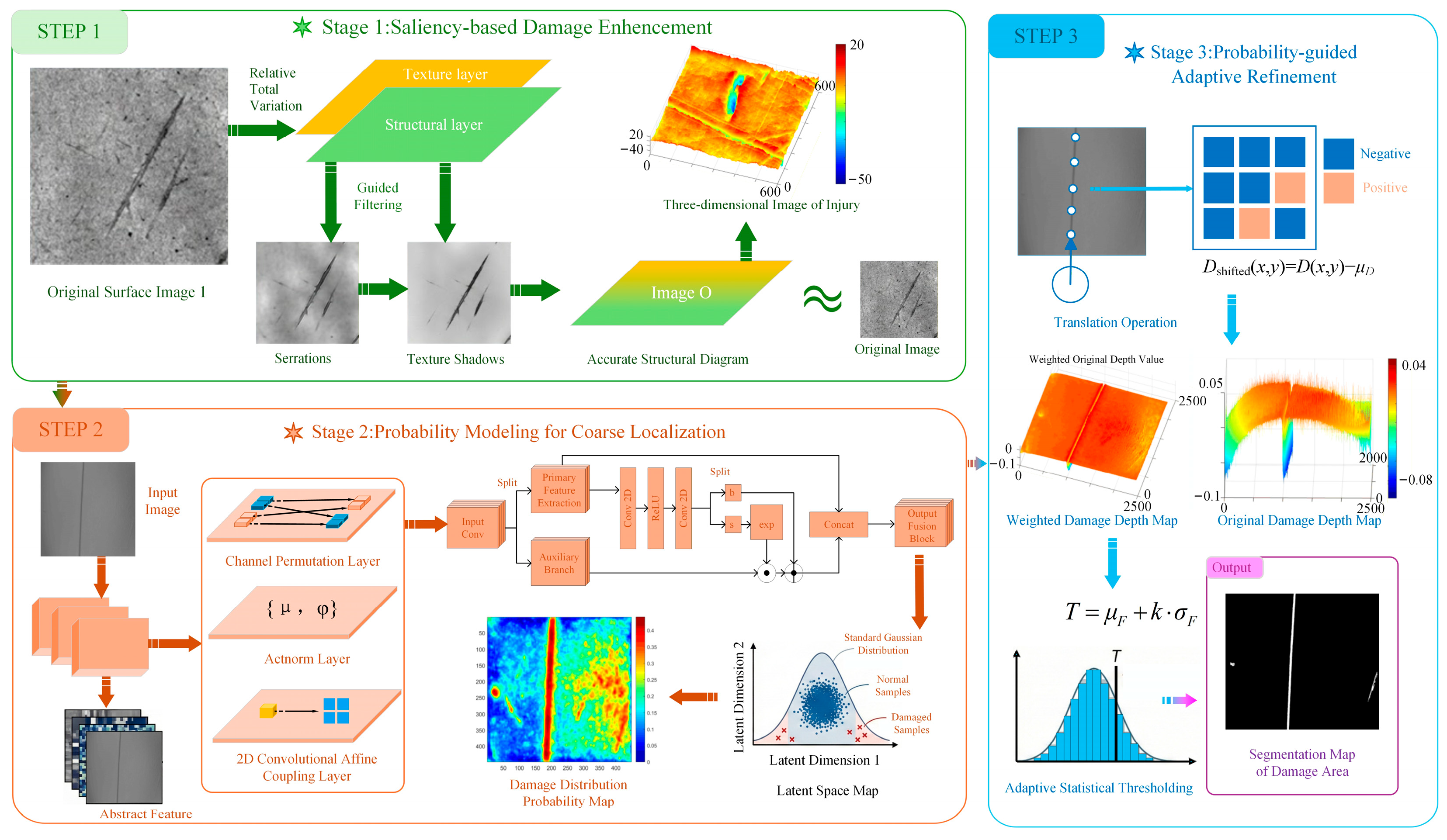
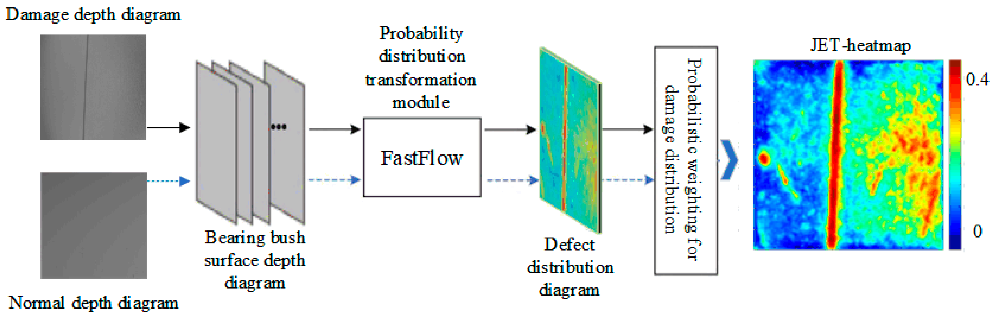
As illustrated in Figure 1, the proposed unsupervised damage detection framework for hydroturbine bearing-pad wear surfaces comprises three main components: saliency-based damage enhancement, anomaly score-based coarse localization, and anomaly score-guided adaptive refinement. First, a salient damage detection module is established based on topography–texture separation to suppress local micro-texture noise and improve the reliability of defect segmentation in large field-of-view depth images. Then, defect-free bearing-pad depth images are utilized to construct a normal reference dataset, and an unsupervised network is adopted to generate anomaly score representations of potential damage regions for coarse localization. Finally, the resulting damage anomaly score distribution is introduced as adaptive weights to fuse depth-based defect cues with morphological processing, thereby achieving self-adaptive refinement of damage regions and supporting subsequent geometric quantification. The detailed methodology is presented in the following sections.

2.2. Salient Damage Detection Based on Morphological Structure–Texture Decomposition

Since the acquired microscopic surface images contain not only regional structural information, such as damaged areas and normal surfaces, but also amplified microscopic surface textures and noise details, accurate detection of damaged regions is severely compromised. Therefore, this section first decomposes the microscopic surface texture and regional structural information by constructing an optimized relative total variation algorithm. Subsequently, the surface-damage region is segmented using an adaptive local thresholding method.

The bearing surface primarily consists of high-frequency detail components (texture and noise) and low-frequency structural components (normal and damaged surface regions). By decomposing and separating the surface texture information, the interference of surface texture noise on damage region detection can be effectively removed. For a surface image I, it can be represented as a linear combination of structure S and texture T, formulated as follows:

$$\mathit{I}=\mathit{S}+\mathit{T}$$

(1)

The structural extraction of bearing surface images refers to extracting the structural image S from the original surface image I. To ensure that the extracted S preserves most of the image’s information features, the L2 norm is used to quantify the degree of conformity between the structural component and the original image. Therefore, the basic model for bearing surface structure S extraction is formulated as follows:

$$\underset{\mathit{S}}{\min }{\displaystyle \frac{1}{2}}{‖\mathit{S}-\mathit{I}‖}^2+\lambda prior$$

(2)

In this equation, the first term is the data fidelity term, which enforces S to approximate the original image I as closely as possible, preserving large-scale structural information while constraining texture components. The second term is the prior term, which incorporates different prior information to regularize the image structure S. The parameter λ balances the weights between the first and second terms. Considering that the Relative Total Variation (RTV) prior can impose different penalty constraints on texture and structure during global optimization, it effectively discriminates between texture and structure, particularly when structural components are interspersed with substantial texture. Therefore, based on the basic model for structure extraction and utilizing RTV, the following surface structure decomposition model is obtained:

$$\underset{\mathit{S}}{\min }{\displaystyle \frac{1}{2}}{‖\mathit{S}-\mathit{I}‖}^2+\lambda \mathrm{RTV}\left(\mathit{S}\right)$$

(3)

In this equation, RTV is the ratio of the Windowed Total Variation to the Windowed Inherent Variation. The relative total variation RTV at pixel p is defined as:

$$\mathrm{RTV}{\left(\mathit{S}\right)}_p={\displaystyle \frac{{\mathrm{F}}_h(p)}{{\mathrm{J}}_h(p)+\epsilon }}+{\displaystyle \frac{{\mathrm{F}}_v(p)}{{\mathrm{J}}_v(p)+\epsilon }}$$

(4)

In this equation, ε is a small constant used to prevent division by zero. F and J represent the Windowed Total Variation (WTV) and Windowed Inherent Variation (WIV), respectively, defined as:

$${\mathrm{F}}_h(p)={\displaystyle \sum _{n\in R\left(p\right)}{\mathrm{g}}_{p,n}\left|{\left({\partial }_h\mathit{S}\right)}_n\right|}$$

(5)

$${\mathrm{F}}_v(p)={\displaystyle \sum _{n\in R\left(p\right)}{\mathrm{g}}_{p,n}\left|{\left({\partial }_v\mathit{S}\right)}_n\right|}$$

(6)

$${\mathrm{J}}_h(p)=\left|{\displaystyle \sum _{n\in R\left(p\right)}{\mathrm{g}}_{p,n}{\left({\partial }_h\mathit{S}\right)}_n}\right|$$

(7)

$${\mathrm{J}}_v(p)=\left|{\displaystyle \sum _{n\in R\left(p\right)}{\mathrm{g}}_{p,n}{\left({\partial }_v\mathit{S}\right)}_n}\right|$$

(8)

In this equation, n represents a pixel within the rectangular neighborhood of pixel p; ${\partial }_h\mathit{S}$ and ${\partial }_v\mathit{S}$ are the partial derivatives of the structural image S in the horizontal and vertical directions, respectively; ${\mathrm{g}}_{p,n}$ is a weighting function related to spatial distance, defined as follows:

$${\mathrm{g}}_{p,n}=\exp \left(-{\displaystyle \frac{{\left(x_p-x_n\right)}^2+{\left(y_p-y_n\right)}^2}{2{\sigma }^2}}\right)$$

(9)

In this equation, σ controls the spatial scale of the rectangular neighborhood; the larger its value, the smoother the resulting structural image S.

However, this method cannot effectively remove texture at structural edges, exhibiting jagged edges or texture shadows. It has a strong dependence on the spatial scale parameter σ, requiring σ to be determined by the scale of the textures in the image. To further address the limitations of the RTV method, guided filtering is employed to smooth the texture noise of the worn surface image I while preserving clear structural edge information, yielding image O. Based on Equations (10) and (11), a more accurate structural image is obtained by enforcing S to approximate O, defined as follows:

$$\underset{\mathit{S}}{\min }{\displaystyle \frac{1}{2}}{‖\mathit{S}-\mathit{O}‖}^2+\lambda \mathrm{RTV}\left(\mathit{S}\right)$$

(10)

$${\mathit{O}}_i=a_k{\mathit{G}}_i+b_k,i\in w_k$$

(11)

In this equation, G is the guidance image, $w_k$ is a rectangular $n\times n$ window centered at pixel k, and $a_k$ and $b_k$ are linear coefficients that remain constant within the local window.

To ensure that image O approximates the original image I, the determination of coefficients $a_k$ and $b_k$ can be formulated as an optimization problem, i.e., minimizing the following expression:

$$\mathrm{E}\left(a_k,b_k\right)={\displaystyle \sum _{i\in w_k}\left[{\left(a_k{\mathit{G}}_i+b_k-{\mathit{I}}_i\right)}^2+\beta a_k^2\right]}$$

(12)

In this equation, ε is a regularization parameter. The corresponding parameter values can be obtained by taking partial derivatives with respect to $a_k$ and $b_k$, respectively:

$${\displaystyle \frac{\partial \mathrm{E}}{\partial a_k}}={\displaystyle \sum _{i\in w_k}\left[2{\mathit{G}}_i\left(a_k{\mathit{G}}_i+b_k-{\mathit{I}}_i\right)+2\beta a_k\right]}=0$$

(13)

$${\displaystyle \frac{\partial \mathrm{E}}{\partial b_k}}={\displaystyle \sum _{i\in w_k}2\left(a_k{\mathit{G}}_i+b_k-{\mathit{I}}_i\right)}=0$$

(14)

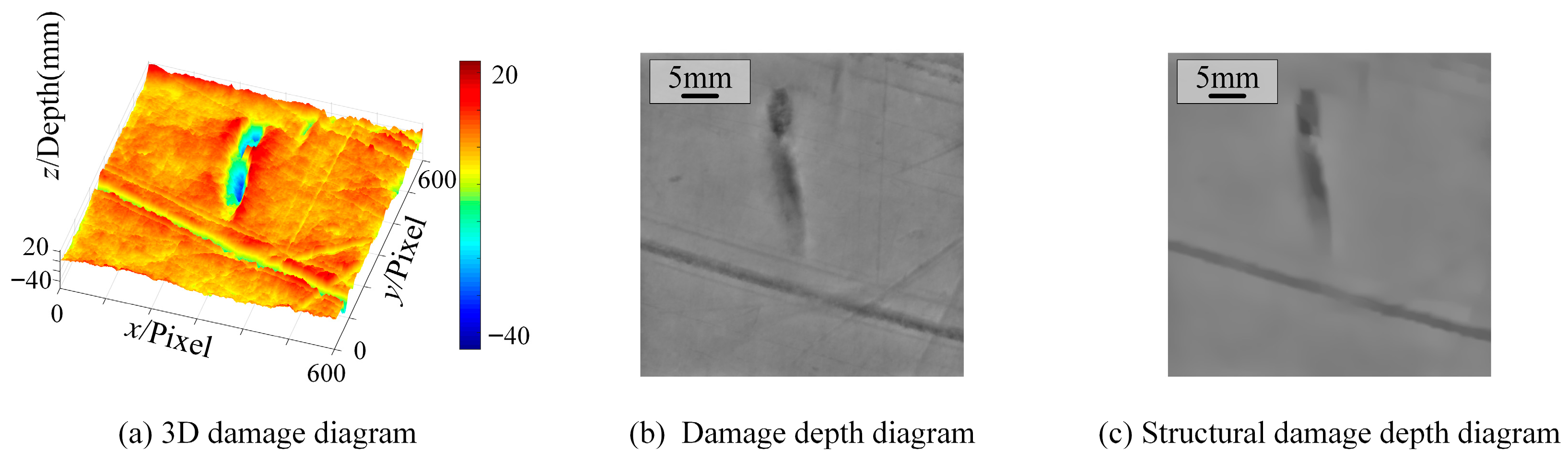
Combining Equations (1)–(14) with the optimization problem-solving method for minimization, the final bearing surface structural image S can be obtained, as shown in Figure 2.

2.3. Anomaly Representation of Deep Surface Damage Areas Based on Unsupervised Learning

Taking the denoised depth image data of the damaged bearing surface under inspection as the research object, a two-dimensional normalizing flow model is employed to map the bearing surface depth image feature data to a standard Gaussian distribution. Since surface-damage regions are discretely distributed outside this distribution, they exhibit higher anomaly scores than normal samples, thereby enabling anomaly score characterization of bearing surface-damage regions. Specifically, the normalizing flow model partitions image features into normal and anomalous intervals that conform to a Gaussian distribution and are easily tractable. A learnable probability density estimation model P, $P=\left\{P_{\theta }:\theta \in \mathsf{\Theta }\right\}$ is utilized to learn parameters θ in the parameter space $\mathsf{\Theta }\left(\theta \right)$ during training, mapping image features to the Gaussian distribution space $z\in P_z\left(z\right)$ through a series of invertible transformations $x\in P_x\left(x\right)$, where $\det \left(·\right)$ denotes the determinant:

$$P_x(x)=P_z(z)|\det ({\displaystyle \frac{\partial z}{\partial x}})|$$

(15)

The log-likelihood function $\log P_x\left(x\right)$ represents the degree of similarity between $P_x\left(x\right)$ and $P_z\left(z\right)$. When the maximum is achieved during the training process $\log P_x\left(x\right)$, the optimal parameter space of P $\mathsf{\Theta }\left(\theta \right)$ is obtained.

$$z=f_{\theta }(x)$$

(16)

$$\log P_x(x)=\log P_z(f_{\theta }(x))+\log |\det ({\displaystyle \frac{\partial f_{\theta }(x)}{\partial x}})|$$

(17)

Since bearing surface defects do not lie within the normal feature distribution space and are discretely distributed outside the $P_z\left(z\right)$ distribution, their $\log P_x\left(x\right)$ is lower. This value can be used to compute the image anomaly score S, where the normalized log-likelihood value is:

$$\overline{P}(x)=\exp (\log P_x(x)-\max [\log P_x(x)])$$

(18)

$$S=\max [\begin{array}{c}{\overline{P}}_x(x)\end{array}]-{\overline{P}}_x(x)$$

(19)

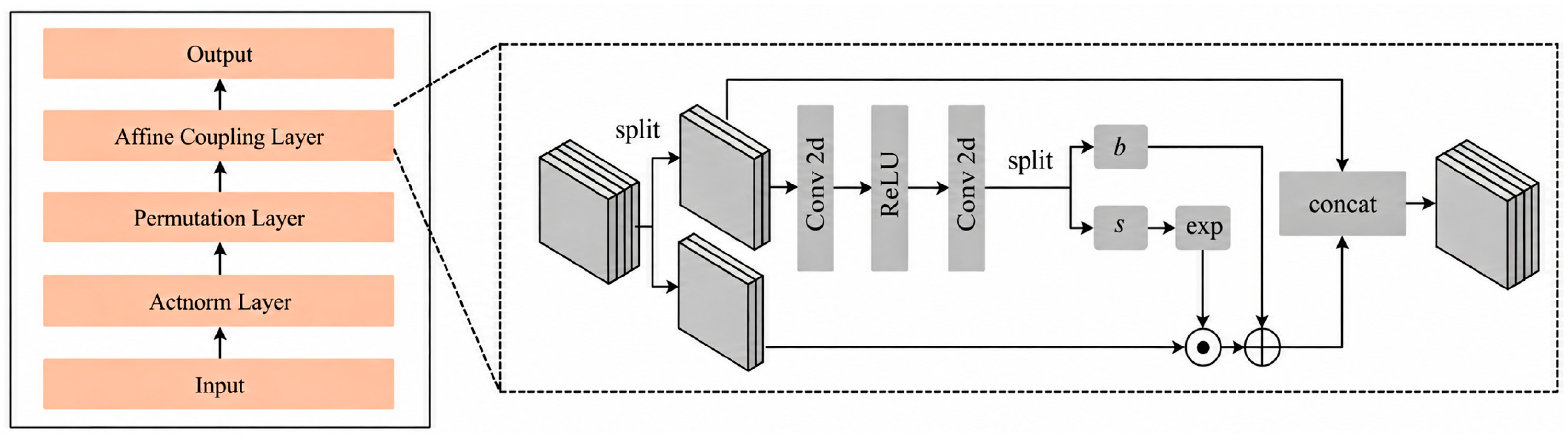
By normalizing the anomaly score S to the range [0,1], the anomaly weight W indicating the likelihood of each pixel belonging to a damaged region in the bearing depth image can be obtained. The normalizing flow model FastFlow in Figure 3 consists of multiple stacked invertible transformation modules, as shown in Figure 4, that map normal features to a standard Gaussian distribution. The Actnorm layer applies affine transformations to each channel to ensure the input data has a distribution with zero mean and unit standard deviation. The channel permutation layer transforms the channel order to mix information flow at each iteration. The affine coupling layer employs two-dimensional convolutional layers to preserve spatial information in the flow model while learning the latent distribution of normal features via affine transformations.

Although the normalizing flow model can effectively distinguish between normal and anomalous features, with anomalous features exhibiting higher anomaly scores, threshold-based methods can identify bearing surface damage defects. However, since the anomaly score distribution only considers anomalous variations in image surface intensity, direct threshold segmentation based on the anomaly score distribution map is prone to over- or under-segmentation when incorporating absolute depth information for accurate judgment. Therefore, this work uses the obtained surface-damage-region anomaly weighting as guidance and further integrates depth information for joint decision-making, thereby achieving accurate segmentation and detection of bearing surface-damage regions.

2.4. Region Detection Based on Joint Anomaly Score Weight and Depth Information

Based on the anomaly score weight map $W\in {\left[0,1\right]}^{H\times W}$ computed by the normalizing flow model, fusion-based judgment is performed by integrating the bearing surface depth information $D\in {ℝ}^{H\times W}$ to achieve more precise damage region segmentation. Specifically, to eliminate baseline drift in the bearing surface depth data, the original depth map D needs to be shifted to zero mean. The depth mean of normal regions is calculated from depth maps of undamaged samples, followed by a translation operation on the entire image:

$$D_{\mathrm{shifted}}(x,y)=D(x,y)-{\mu }_D$$

(20)

In the shifted depth map D, positive values indicate protruding damage, while negative values indicate depressed damage. This strategy helps amplify the absolute depth values of protrusions and depressions during damage-region-weight-guided processing, laying the foundation for precise damage segmentation.

To integrate anomaly score and depth anomaly information, for each pixel, the anomaly score weight W(x, y) is element-wise multiplied with the depth map and then multiplied by the exponential of the probability weight, generating the fused depth map:

$$F(x,y)=W(x,y)\cdot D_{\mathrm{shifted}}(x,y)\cdot \exp \left(\alpha \cdot |D_{\mathrm{shifted}}(x,y)|\right)$$

(21)

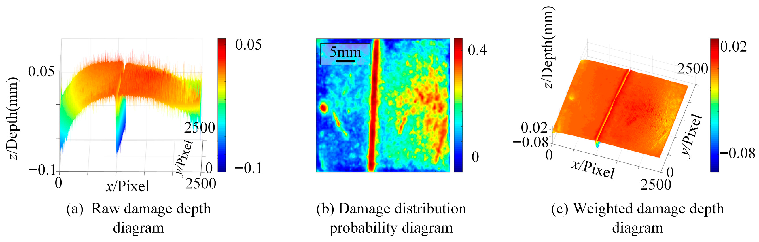
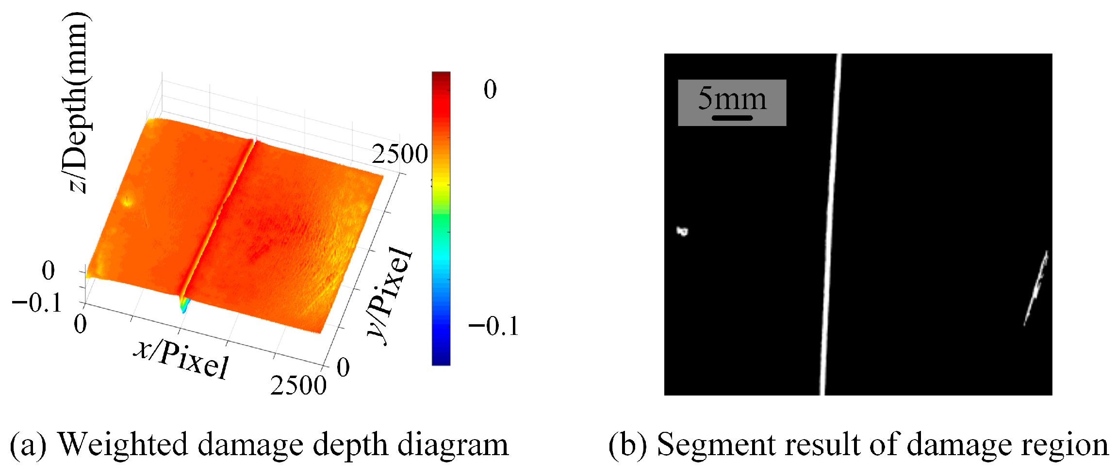
where α is the depth weighting coefficient (default value 1), by adjusting α, the contributions of probability and depth information can be balanced. The exponential function is used to amplify the signal in regions with significant depth anomalies, while low-anomaly score regions (W ≈ 0) are suppressed. The fused depth map F incorporates both statistical anomalies and physical depth information, significantly improving the signal-to-noise ratio (SNR) of damage regions, as shown in Figure 5. The inclusion of the exponential term in Equation (21) is far from arbitrary. It functions as a selective non-linear amplifier: it aggressively boosts the signal in regions with high anomaly confidence (large W) while simultaneously flattening low-confidence background noise (W ≈ 0). Physically, this non-linear mapping is essential for pulling out the subtle, shallow depth gradients that characterize early-stage bearing wear, thereby avoiding the common pitfall of under-segmentation.

Based on the fused feature map F, adaptive statistical thresholding is applied to segment the weighted damage depth map, generating a binary damage mask $M\in {\left[0,1\right]}^{H\times W}$. The threshold T can be determined as follows:

$$T={\mu }_F+k\cdot {\sigma }_F$$

(22)

where μ_F and σ_F are the mean and standard deviation of F, respectively, and k is an empirical coefficient. The segmentation formula is:

$$M(x,y)=\left\{\begin{array}{ll}1\hfill & \mathrm{if}F(x,y)\ge T\hfill \\ 0\hfill & \mathrm{otherwise}\hfill \end{array}\right.$$

(23)

We also implemented a strict dimensional conversion protocol to guarantee the physical validity of our final measurements. While the 2D spatial plane (X and Y coordinates) is uniformly resized to 256 × 256 pixels to fit the model’s input requirements, we carefully record the spatial scaling factor. More importantly, the depth values (the Z coordinate) are completely decoupled from this resizing and remain strictly in their raw physical metric scale (mm). Once the segmentation is complete, applying the inverse scaling factor maps the pixel-based area directly back to real-world physical dimensions.

Based on Equations (20)–(23), the continuous anomaly score distribution can be transformed into discrete damage region labels. Combined with morphological image operations, including opening, closing, and connected component filtering, the final segmentation map of bearing damage regions can be obtained, as shown in Figure 6.

3. Verification

3.1. Description of Image Sample Data

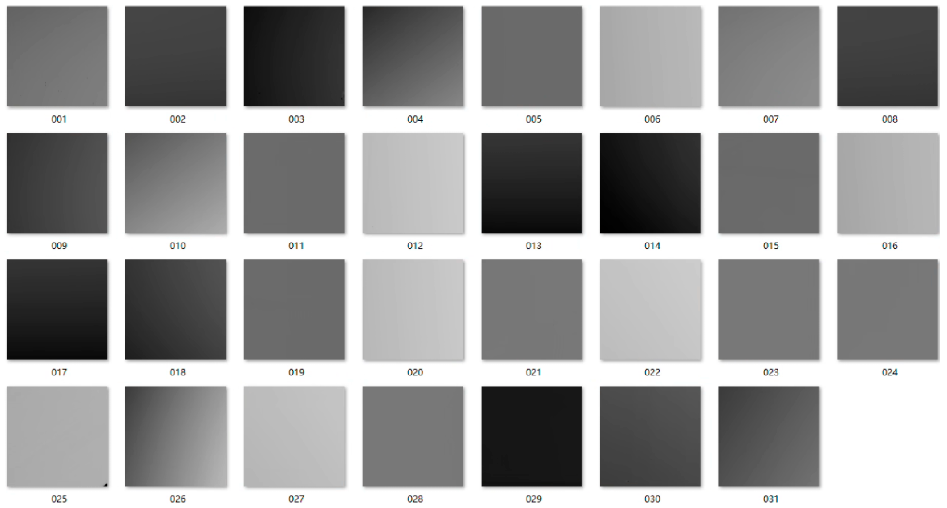
To further validate the effectiveness of the proposed method, this section first constructs structured-light depth maps corresponding to the morphology of bearing surface samples without damage, and uses them as a sample dataset to train an unsupervised anomaly representation model for bearings. As shown in Figure 7, the experiment collected 31 defect-free real-surface samples as the normal training set. These samples encompass surface texture features of various critical components, including guide bearings, water seal blocks, water seal wear-resistant plates, and thrust bearings. While bearing pads are our primary focus, we deliberately included other hydroturbine friction components (such as water seal blocks) in the normal reference dataset. Because these components share nearly identical material compositions, Babbitt metal machining signatures, and tribological wear environments, their inclusion provides the model with a much richer understanding of ‘normal’ machined background textures. Furthermore, to absolutely eliminate any potential for data leakage, we rigidly partitioned the dataset at the physical sample level. Training patches were extracted exclusively from pristine components, whereas the testing set was built entirely from physically distinct, damaged components, ensuring absolute zero spatial overlap. To meet the model input requirements and ensure effective feature extraction, all depth images underwent preprocessing, including uniform cropping and resizing to 256 × 256 pixels. This dataset not only contains background textures generated by different materials and manufacturing processes, but also covers surface morphologies under various lighting conditions, effectively testing the model’s robustness under complex operating conditions.

3.2. Anomaly Characterization of Damage Distribution

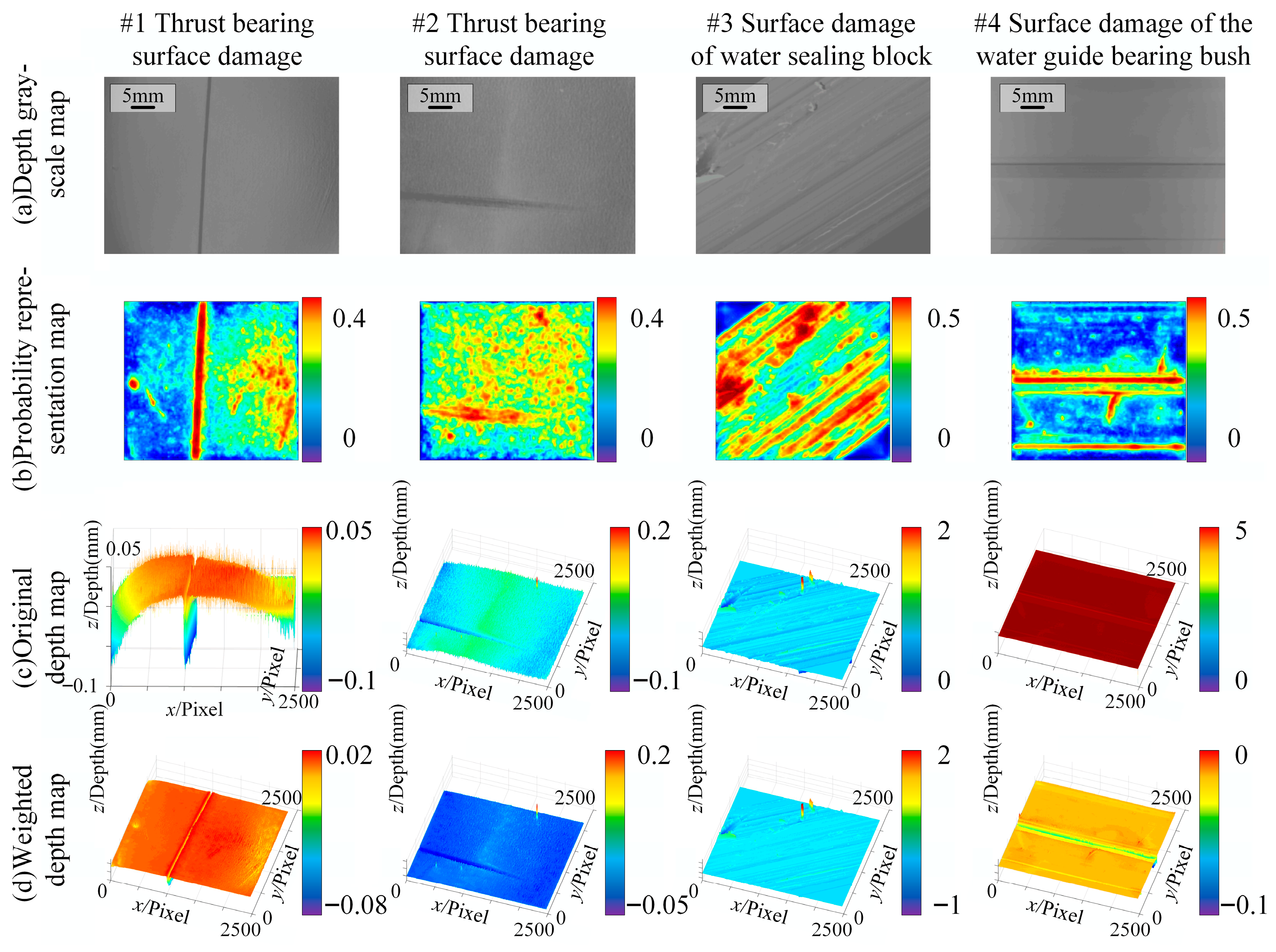
The FastFlow model training parameters were configured as follows: the model input resolution was set to 256 × 256, the Adam optimizer was employed for parameter updates, the initial learning rate was set to 0.001, and the weight decay was set to 0.00001. To ensure the model fully converged and accurately learned the distributional characteristics of normal samples, the number of training epochs was set to 500 and the batch size to 32. During training, only the aforementioned 31 normal samples were used, without introducing any synthetically generated anomalous data, to validate the effectiveness of unsupervised learning. Based on this, scratches and pit damage on real surfaces were selected for depth information extraction, obtaining the corresponding depth maps and segment results as shown in Figure 8.

Figure 8 presents the typical anomaly score characterization and weighted depth results for real bearing surfaces. Specifically, Figure 8a shows the depth grayscale maps, which intuitively reflect surface height information through grayscale values and clearly present the geometric features of damage, such as scratches and pits. However, due to interference from complex background textures, the contrast between some damaged areas and normal regions is relatively low. Figure 8b displays the anomaly characterization maps generated by the normalizing flow model, which visualize the anomaly score distribution as heatmaps and successfully localize the main damage regions. However, minor false detections still occur for subtle textures. Figure 8c shows the original depth maps after shift processing, which makes the depth differences in damage regions more pronounced, providing clear boundaries between normal regions near zero values and anomalous regions that significantly deviate. Figure 8d presents the weighted depth maps, which effectively enhance the true damage signals by fusing anomaly weights and depth information. By correcting and optimizing damage regions using weighted depth maps, comprehensive results are demonstrated that incorporate both anomaly score and depth information.

3.3. Bearing Damage Detection Evaluation

Based on the weighted depth maps, the real bearing surface-damage region was further detected by integrating anomaly score weights and depth information, as shown in Figure 9. To comprehensively evaluate segmentation performance, the project employed surface area error E_s and volume error E_v. To establish an uncompromising and authoritative baseline, the ground-truth area (S_g) and volume (V_g) were not merely estimated. Instead, a senior metrology engineer manually delineated the defect boundaries point-by-point directly on the raw, uncompressed 3D point cloud data using high-precision commercial metrology software (MPSizectors SDK software, version 2.47).

$$E_S={\displaystyle \frac{\left|S_m-S_g\right|}{S_g}}\%$$

(24)

$$E_V={\displaystyle \frac{\left|V_m-V_g\right|}{V_g}}\%$$

(25)

where S_m and S_g are the measured area and the actual area, respectively; V_m and V_g are the measured volume and the true volume, respectively.

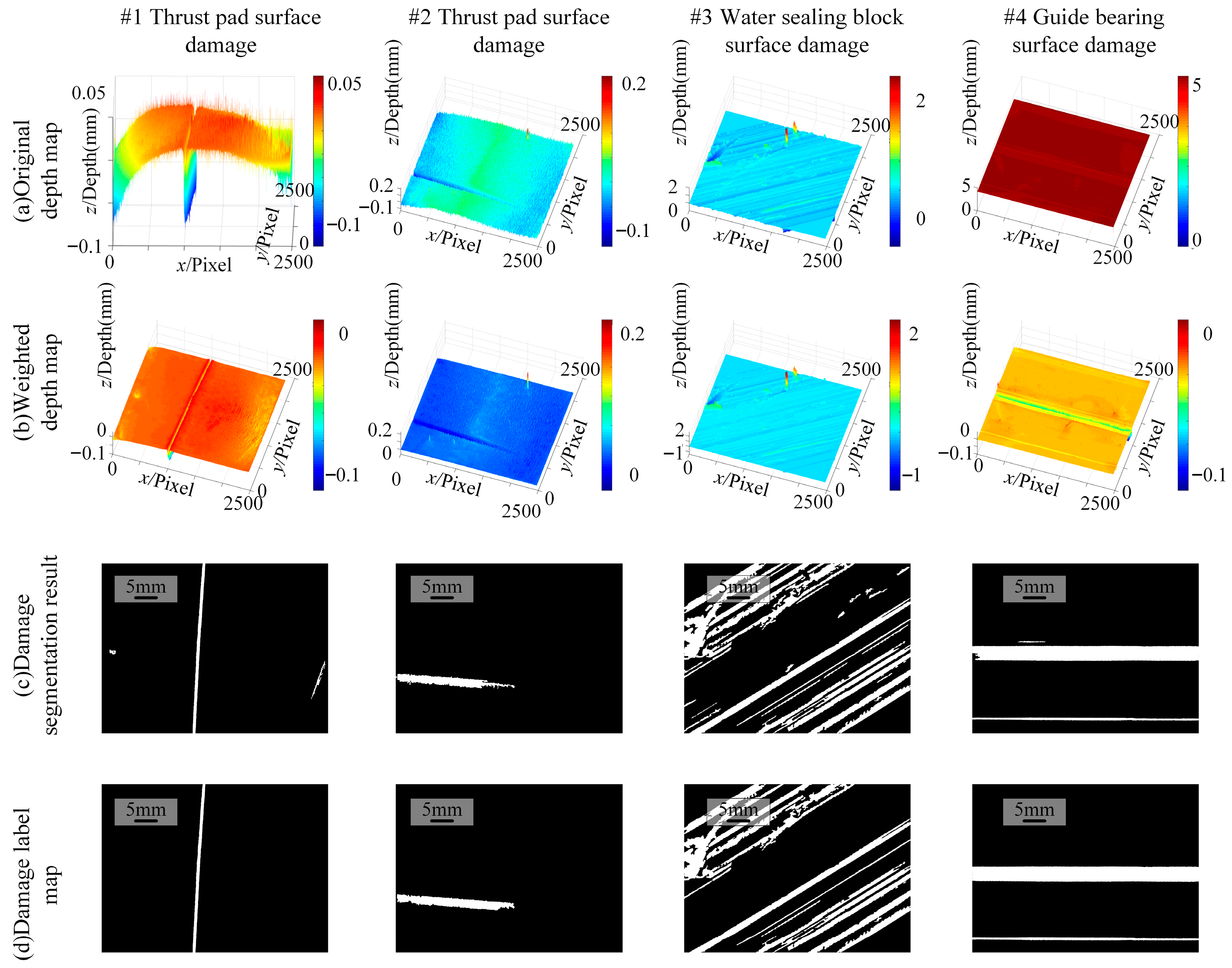
Figure 9 intuitively demonstrates the segmentation pipeline and comparisons of results for four typical bearing surface damage cases.

Row(a) represents the original depth maps: these display the raw three-dimensional morphology data acquired from thrust bearing, water seal, and guide bearing surfaces. Notable interference from machining tool marks is evident in the background of samples such as water seal blocks, and the scratches in the thrust bearing surface damage samples are relatively shallow, presenting significant identification challenges.

Row(b) represents the weighted depth maps: after anomaly weighting processing, background noise is significantly suppressed, while depth features of damage regions are enhanced. In particular, deep pits and groove features in the thrust bearing surface damage and water guide bearing samples become more prominent.

Row(c) represents the damage segmentation results: these show the binarized results obtained by segmenting the weighted maps using the proposed algorithm. The algorithm successfully extracts the main damage morphologies from complex backgrounds. For damage in water-seal block surfaces with large-area, complex, textured backgrounds, the algorithm maintains good edge integrity. For subtle scratches on thrust bearing surfaces, it also achieves continuous detection.

Row(d) represents the damage label maps: these are manually fine-annotated ground truth masks. Comparing (c) and (d) reveals that the segmentation results of the proposed method are highly consistent with the ground truth labels, with only minor differences at extreme edges, demonstrating the superiority of this detection method in localization accuracy and shape reconstruction.

The structured light measurement results in

Table 1. Quantitative results of the segmented damage regions.

	#1	#2	#3	#4
Real surface area (mm2)	18.1827	29.5339	300.7077	138.7734
Surface area error	14.76% ± 2.10%	11.75% ± 1.85%	7.39% ± 1.20%	3.67% ± 0.85%
Measured Area (mm2)	20.89 ± 0.45	26.06 ± 0.62	322.93 ± 4.15	133.68 ± 1.20
Real Volume (mm3)	1.0979	1.3048	26.1533	4.2554
Measured Volume (mm3)	1.178 ± 0.052	1.205 ± 0.081	27.126 ± 0.850	4.211 ± 0.110
Volume Error (%)	7.24% ± 1.15%	7.66% ± 1.22%	3.72% ± 0.85%	1.03% ± 0.35%

show that volume measurement accuracy is generally superior to surface area measurement. Sample #4 (water guide bearing) achieves a mean volume error of 1.03% ± 0.35%, while sample #3 (water seal sealing surface) maintains a mean surface area error of 7.39% ± 1.20%, with all measurement errors controlled within 15%. Particularly noteworthy is that the system maintains a 7.24% ± 1.15% volume measurement accuracy for minute volumes at the 1 mm³ level (sample #1), while for large-scale damage exceeding 300 mm² (sample #3), both mean surface area and volume errors remain below 8%. This fully validates the reliability and engineering applicability of the structured light measurement system for damage detection across different scales, meeting the project’s technical requirements.

3.4. Ablation Study and Hyperparameter Sensitivity

To truly understand the value each component adds to our framework, we conducted a step-by-step ablation study (see

Table 2. Ablation study on the proposed framework components.

Configuration	Pixel-F1 Score
Baseline FastFlow	27.24%
FastFlow + RTV	65.80%
FastFlow + depth-weighted fusion (without RTV)	65.64%
Proposed	92.41%

). If we rely solely on the baseline FastFlow model, the system is quite capable of detecting general anomalies, but it fundamentally struggles with precise boundary delineation, scraping by with a Pixel-F1 Score of only 27.24%.

To isolate the contribution of the fusion module, an intermediate configuration consisting of FastFlow and depth-weighted fusion (without RTV) was evaluated, yielding a Pixel-F1 Score of 65.64%. This demonstrates that while physical depth constraints improve boundary delineation over the baseline, removing the high-frequency interference via RTV is still crucial for maximizing segmentation accuracy.

The picture changes dramatically as we introduce our tailored modules. First, by applying the RTV topography–texture decomposition, we effectively strip away the high-frequency distraction of machining tool marks. This cleaner input immediately boosts the Pixel-F1 Score to approximately 65.80%. Finally, the integration of our depth-weighted fusion (Equation (21)) bridges the crucial gap between a fuzzy probability heatmap and a crisp physical boundary, driving the Pixel-F1 Score to a peak of 92.41%.

Additionally, a hyperparameter sensitivity analysis on the depth weighting coefficient (α) and the threshold coefficient (k) confirmed the model’s robust operational window. We found that the Pixel-F1 Score comfortably remains above 88.0% as long as α ∈ [0.8,1.2] and k ∈ [2.5,3.5]. Our default setup (α = 1.0, k = 3.0) hits the sweet spot for filtering noise while protecting shallow wear edges, proving that the framework does not require fragile, extreme fine-tuning to perform well in practice.

3.5. Benchmarking Against SOTA Algorithms

A true test of any proposed method is how it stands up against current State-Of-The-Art (SOTA) benchmarks. We evaluated our framework against PaDiM [22] and PatchCore [25], two highly respected unsupervised anomaly detection models known for their robust feature-memory architectures (see

Table 3. Quantitative performance comparison against contemporary SOTA models.

Method	Image-Level AUROC	Pixel-Level AUROC	Pixel-F1 Score
PaDiM [22]	96.50%	89.40%	72.10%
PatchCore [25]	99.10%	92.30%	78.50%
Proposed Method	100%	96.85%	92.41%

). To ensure a fair and rigorous comparison, the performance metrics for PaDiM and PatchCore presented in Table 3 were obtained through an in-house re-implementation applied directly to our custom depth dataset. Both SOTA models were subjected to a unified preprocessing pipeline identical to our proposed framework. The models were trained exclusively on the same 31 defect-free reference samples. For feature extraction, a WideResNet-50 backbone was employed for both PaDiM and PatchCore, with default hyperparameter settings maintained as originally reported in their respective literature.

Quantitatively, PaDiM and PatchCore both deliver excellent image-level classification. However, when it comes to the rigorous task of pixel-level shape delineation (Pixel-F1 Score), they plateau at 72.10% and 78.50%. Our proposed method easily overtakes these baselines, maintaining a flawless 100% Image-level AUROC while pushing the Pixel-F1 Score to an impressive 92.41%.

The underlying reason for this performance gap is clear: while standard SOTA models like PatchCore are exceptional at finding deep feature discrepancies in 2D RGB images, they trip up on the unique physical characteristics of large-field-of-view depth images. To these standard algorithms, the shallow depth gradients of early-stage abrasive wear and the heavy background machining textures often look like indistinguishable ‘out-of-distribution’ noise. By explicitly untangling topography from texture beforehand and enforcing a rigid depth-weighted fusion constraint, our method ensures the final output is not just an abstract heatmap, but a structurally continuous, physically meaningful geometric mask.

3.6. Tribological Interpretation and Maintenance Decision-Making

Ultimately, extracting highly precise geometric features is only half the battle; the real engineering value lies in translating these numbers into actionable maintenance decisions. By closely examining parameters like surface area (S) and the volume-to-area ratio (V/S, which proxies average depth), our framework allows engineers to inversely deduce the specific lubrication failure mode at play. (1) Abrasive Wear and Contamination Monitoring: Monitoring: for example, when a defect shows a high V/S ratio—taking the form of deep, narrow, and heavily directional linear grooves (like those in Samples #1 and #2)—it is a classic fingerprint of lubricant contamination. This morphology tells us that hard particulate contaminants have breached the bearing-rotor clearance and are actively acting as third-body abrasives. From a maintenance perspective, this is a clear early warning: rather than immediately tearing down the turbine, operators know to proactively filter the oil and inspect the sealing systems. (2) Adhesive Wear and Hydrodynamic Oil Film Rupture: Cconversely, broad damage zones with a large area but a shallow depth profile (as seen in Sample #3) tell a very different story. This wide ‘scuffing’ strongly indicates a localized rupture of the hydrodynamic oil film. Whether caused by an excessive load spike or a thermal drop in oil viscosity, the fluid film has failed, dragging the system into boundary lubrication and severe metal-to-metal contact. This scenario dictates a much more urgent maintenance response, potentially requiring an immediate unit shutdown and bearing-pad repair to prevent catastrophic seizure.

3.7. Experimental Comparison and Performance Evaluation

To systematically validate the effectiveness and superiority of the proposed framework, comparative experiments were conducted against two baseline categories: traditional segmentation methods represented by Otsu Thresholding [8,19] and the standard Basic FastFlow model [12,13]. To comprehensively assess detection performance, three standard metrics are adopted: Image-level AUROC, Pixel-level AUROC, and Pixel-F1 Score. The mathematical definitions of these metrics are based on the confusion matrix elements: True Positive (TP), False Positive (FP), False Negative (FN), and True Negative (TN). Image-level AUROC and Pixel-level AUROC evaluate the model’s discriminative ability across various thresholds based on the Area Under the Receiver Operating Characteristic Curve (AUROC), plotting the True Positive Rate (TPR = TP/(TP + FN)) against the False Positive Rate (FPR = FP/(FP + TN)). Specifically, Image-level AUROC assesses the accuracy of classifying defective samples versus defect-free samples, while Pixel-level AUROC evaluates the precision of defect localization at the pixel level. Regarding the Image-level AUROC evaluation reported in Table 3 and

Table 4. Quantitative performance comparison of different defect detection methods.

Method	Image-Level AUROC	Pixel-Level AUROC	Pixel-F1 Score
Otsu	64.50%	58.42%	15.30%
FastFlow	100%	91.60%	27.24%
Proposed	100%	96.85%	92.41%

, the test set was meticulously constructed to ensure zero spatial overlap with the training data. The test set comprises 4 positive (defective) samples and 12 negative (defect-free) samples drawn from physically distinct bearing components. The achievement of a 100% Image-level AUROC across the models is primarily attributable to the distinct, macroscopic topological deviations present in our specific test samples, combined with the relatively constrained size of the testing set. While this confirms the models’ absolute capability to flag severe structural anomalies in this specific sample pool, we acknowledge that expanding the dataset in future work will be necessary to establish broader statistical significance. To further assess the segmentation quality and the consistency of the defect morphology, Pixel-F1 Score is employed. It is the harmonic mean of Precision (TP/(TP + FP)) and Recall (TP/(TP + FN)). A higher Pixel-F1 Score indicates that the segmented defect region highly overlaps with the ground truth without significant over-segmentation or under-segmentation. The quantitative comparison results among the traditional method, the basic deep learning model, and the proposed framework are summarized in Table 4.

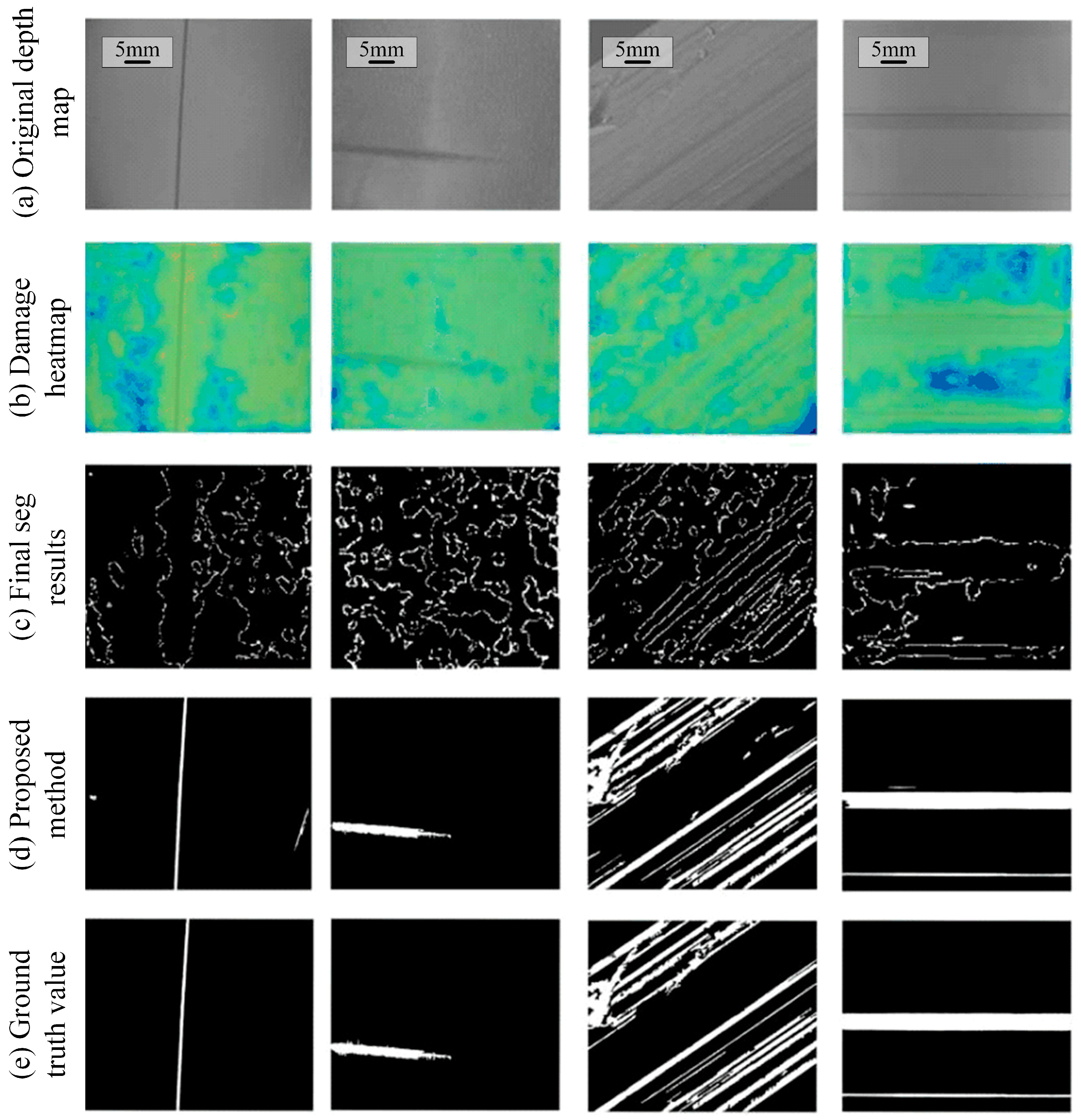
As shown in Table 4, the traditional Otsu method performs poorly in complex texture scenarios. It yields an Image-level AUROC of only 64.50% and a Pixel-level AUROC of 58.42%, indicating a limited ability to distinguish between defective and defect-free surfaces. This poor performance is further reflected in its extremely low Pixel-F1 Score of 15.30%. Visual inspection (Figure 10c) confirms that global thresholding fails to distinguish between machining tool marks and actual wear defects, leading to severe false positives and a noisy segmentation map.

In contrast, the Basic FastFlow model demonstrates strong anomaly scoring capabilities, achieving a perfect Image-level AUROC of 100% and a commendable Pixel-level AUROC of 91.60%. However, without physical depth guidance, its segmentation boundaries remain imprecise, resulting in a relatively low Pixel-F1 Score of 27.24%. This suggests that while the model can detect anomalies, it struggles to accurately delineate defect shapes, often producing under-segmented or over-smoothed regions.

The proposed method significantly overcomes these limitations by integrating depth-weighted fusion. It maintains a perfect Image-level AUROC of 100% while boosting the Pixel-level AUROC to 96.85%, representing a substantial improvement of 38.43% over the traditional Otsu method. Most critically, the introduction of Adaptive Statistical Thresholding dramatically increases the Pixel-F1 Score to 92.41%. This high score confirms that the proposed postprocessing strategy successfully transforms coarse anomaly maps into high-precision segmentation masks, effectively addressing the noise and boundary issues observed in the baseline methods.

Although the proposed method introduces additional preprocessing and fusion steps, the increase in inference time is marginal. This speed still supports a processing rate of approximately 24 frames per second, fully satisfying the real-time requirements for offline industrial inspection. The visual comparison in Figure 10 further corroborates the quantitative data. Row (c) shows that the Basic FastFlow and Otsu results contain varying degrees of noise or fragmented segmentation. Row (d) presents clean, continuous defect regions that highly overlap with the Ground Truth in Row (e). Specifically, for the subtle scratches on the thrust bearing (Column 2) and the heavy-texture water seal surface (Column 3), the proposed method is the only one that achieves both noise suppression and structural integrity.

4. Conclusions

This paper addresses the critical challenges of fine-scale texture interference and the scarcity of defect annotations in hydroturbine bearing-pad wear detection by proposing an unsupervised detection framework guided by local anomaly score distributions. By integrating topography-texture separation with deep anomaly score modeling, the proposed methodology achieves quantitative characterization of wear geometry without relying on pixel-level defect labels. The main contributions and findings of this study are summarized as follows:

(1)

Robust Feature Enhancement via Topography-Texture Separation: To mitigate the interference of machining tool marks and micro-texture noise in large field-of-view depth images, a topography-texture decomposition module based on Relative Total Variation optimization was constructed. This mechanism effectively separates high-frequency background noise from low-frequency structural damage information, significantly enhancing the saliency of potential defect regions and providing high-quality input data for subsequent anomaly detection.

(2)

Unsupervised anomaly score Characterization: A normalizing flow-based network was employed to achieve unsupervised anomaly score characterization of bearing surface damage. Unlike supervised paradigms that require extensive defect-free samples, this model constructs a robust normal distribution using only a limited set of defect-free reference samples. It successfully generates dense anomaly score distribution maps that reflect the severity of anomalies, thereby overcoming the challenges posed by unpredictable defect morphologies in industrial scenarios.

(3)

High-Precision Quantitative Assessment: An adaptive segmentation strategy was developed by fusing damage-anomaly weighting with physical depth information. Despite these highly encouraging results, we must acknowledge the limitations of the current study. For one, our dataset—comprising 31 pristine samples and 4 test samples—is admittedly modest in scale, which naturally introduces some statistical variance into the evaluation metrics. Expanding this dataset is a priority for more robust statistical validation. Furthermore, our current tests were conducted on static samples in a controlled lab environment. The actual reality inside a hydroelectric powerhouse—complete with intense mechanical vibrations, severe oil contamination, and vast sample diversity—is exponentially more complex. Bridging this gap by adapting the algorithm for dynamic, in situ online monitoring remains our primary focus for future work.

In summary, the proposed framework provides a reliable, automated, and quantitative solution for hydroturbine bearing-pad inspection, significantly reducing the dependence on expert experience and labeled data. Future work will focus on expanding the sample database to cover a broader range of operating conditions and on deploying this algorithm on edge computing devices for real-time online monitoring.