Investigating Film Thickness and Friction of an MR-Lubricated Journal Bearing

Abstract

Magnetorheological (MR) fluids are frequently reported to have potential as lubricants for hydrodynamic bearings operating at high loads, but no comprehensive effort has been made to investigate their performance under a variety of operating conditions. This paper, therefore, presents an extensive experimental and numerical investigation of an MR-lubricated hydrodynamic journal bearing subjected to different loads and magnetic fields, and compares these results to those of an oil-lubricated bearing. It is shown that by increasing the magnetic field strength, the performance characteristics of the bearing can be changed from low hydrodynamic friction and a high transition speed to high hydrodynamic friction and a low transition speed. Furthermore, it was found that the way in which these characteristics scale with increasing load differs for the MR- and oil-lubricated bearings. With MR lubrication, the relative change in characteristics with the application of a magnetic field is smaller at higher loads, due to the strong shear-thinning rheology of MR fluids. To include these effects in the model, a basic relation for the apparent MR viscosity as a function of shear rate, temperature, and magnetic field strength is introduced. Finally, the bearing was made from a polymer to improve wear resistance under MR lubrication, but a comparison with a Reynolds equation-based numerical model indicates possible performance degradation due to shape errors, which is a known issue with this bearing material.

1. Introduction

A hydrodynamic journal bearing is defined by its lubricating film, which separates the two surfaces and thereby minimises friction and prevents wear. The thickness of this film depends on various factors like the geometry, the speed of the shaft, and the properties of the lubricant that is being used. A very important lubricant property is the viscosity, with higher viscosity leading to thicker films but also to higher friction, and vice versa. Viscosity is an inherent property of a standard lubricating oil, but with ‘smart’ lubricants like magnetorheological (MR) fluids, it is possible to actively control the apparent viscosity with the application of an external magnetic field.

An MR fluid consists of a base oil with a large number of iron microparticles in suspension (generally around 20 vol%). In general, the MR fluid responds like a standard (albeit strongly shear-thinning) lubricant, but with the application of a magnetic field, the particles in the fluid will magnetite, and will form chain-like structures along the magnetic field lines. These structures impede the flow of the base oil, manifesting as an increase in the effective viscosity on the macro scale. The magnetic field also enhances the shear-thinning characteristics, with higher stresses leading to the breakage of the structures and therefore to progressively smaller viscosity increases. In contrast, lower stresses will strengthen the particle structures, eventually preventing the flow of base oil completely and turning the fluid into something resembling a viscoplastic solid. Finally, all of these magnetically induced effects are fully reversible, removing the magnetic field will result in the original suspension in only a few milliseconds [1,2].

In the past, the controllable viscosity of MR fluids has been used mainly to construct active dampers and brakes, but other applications have also been investigated, such as actuators, haptic devices, and magnetic metamaterials [3,4,5,6]. In addition, some research has been conducted on the use of MR fluids as lubricant in hydrodynamic (journal) bearings. Due to the complicated non-Newtonian characteristics of MR fluids, a relatively large number of researchers have focused on modelling these bearings numerically. A number of viscosity models have been identified that can describe these non-Newtonian characteristics with reasonable accuracy, most notably the Bingham plastic and Herschel–Bulkley models [7]. These viscosity models can then be combined with either the Navier–Stokes equations for a full 3D CFD model [8] or with a variant of the Reynolds equation for a simpler 2D or even 1D model [9,10]. Several general journal bearing case studies have been created where these types of models were used to investigate the effects of MR lubrication [11,12,13]. More focused studies can be found as well, for example, ones investigating dynamic behaviour [14,15] or the influence of surface textures [16], surface roughness [17], or temperature [18]. In general, it has been observed that an increase in lubricant viscosity due a stronger magnetic field leads to thicker films (or equivalently, a reduction in the transition speed) but also to higher friction.

Several experimental investigations into MR lubrication in bearings have also been carried out, but these are more rare. In one of the earliest experimental papers, an MR-lubricated hydrostatic bearing was successfully designed to achieve a constant film thickness independent of load by varying the magnetic field strength [19,20]. Several experiments with journal bearing setups were then performed, confirming the general findings of numerical research that stronger fields lead to both thicker films and higher friction [15,21,22,23]. Some of these researchers have suggested that the active control of the magnetic fields using electromagnets could be a way of achieving both thick films at low speeds, and low friction at high speeds, by reducing the strength of the magnetic field at higher speeds [22]. Similarly, the use of local magnetic fields has been proposed as a way of minimising the friction increase by only magnetising the film where an increase in viscosity has the largest effect on film thickness (near minimum film), instead of magnetising the entire film [24,25]. Two investigations have looked into this concept and have compared the performance of MR fluid with that of standard (Newtonian) lubricating oils. The first used a very strong local magnetic field with a standard MR fluid, and found that the resulting film thickness and friction were both still higher than with the standard lubricating oil [26]. On the other hand, the second used a weaker magnetic field and a fluid with fewer particles (reducing the magnitude of the viscosity increase), and found the MR-lubricated bearing to have lower friction than the oil-lubricated bearing, but also a higher transition speed (equivalent to a lower film thickness) [27]. Both suggested that the fluid and magnetic field should be optimised further.

In summary, the use of MR fluid as a lubricant for hydrodynamic (journal) bearings has gotten some (mostly numerical) attention in the literature. Generally, it has been found that the increase in viscosity due to the magnetic field will not only increase the film thickness, and thus reduce the transition speed, but will also result in higher friction compared to standard lubricants. However, while some suggestions have been made for possible ways to improve these bearings and obtain performance superior to that of an oil-lubricated bearing, there has not yet been a comprehensive effort to find out under which operating conditions this would actually be possible, if at all. This work therefore presents an extensive experimental and numerical investigation into the performance of an MR-lubricated journal bearing under different loads and with different magnetic fields, and compares this to the same bearing lubricated with a standard oil.

2. Materials and Methods

In this study, experiments were performed with a custom hydrodynamic journal bearing setup, lubricated either with a reference oil or a magnetorheological (MR) fluid. These results were compared with those of a numerical model. This section will first introduce the experimental setup and experimental procedures, and will then discuss the model.

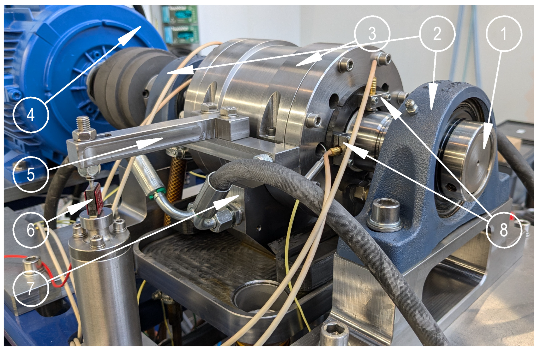
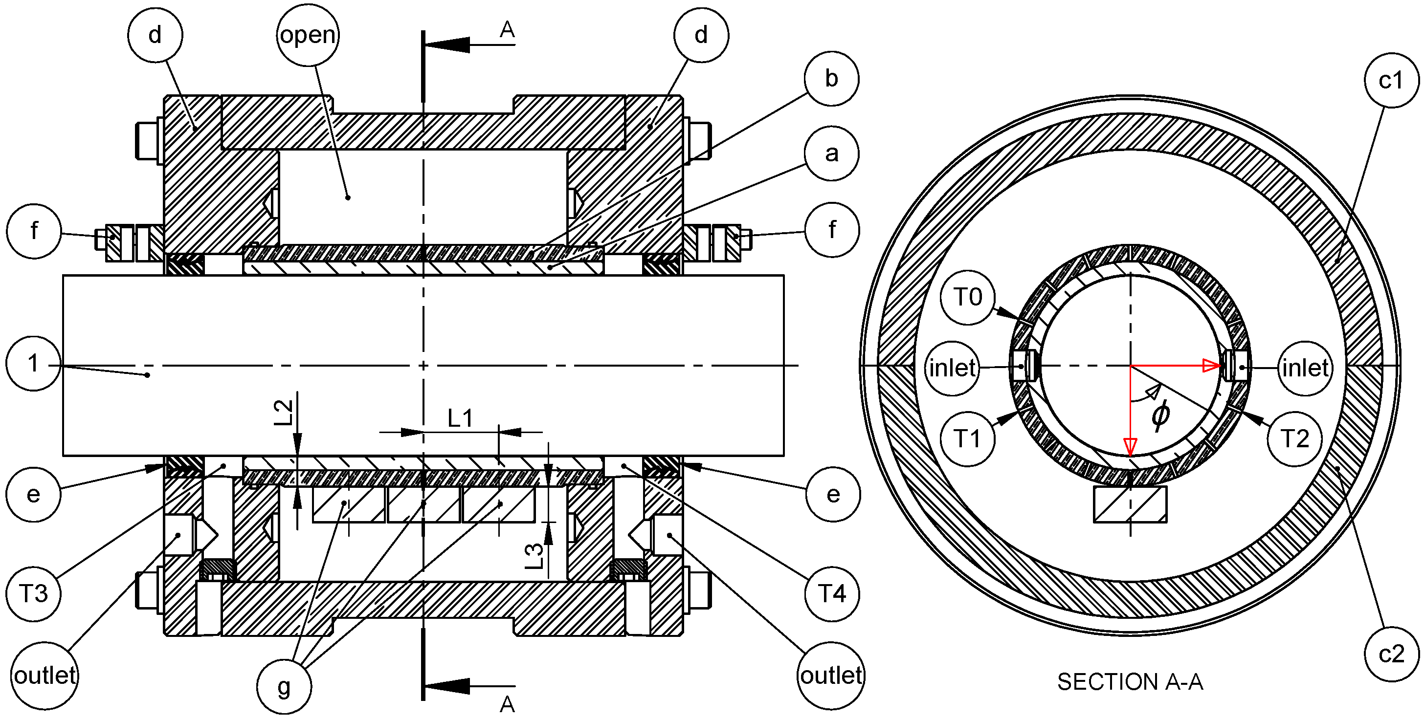
2.1. Experimental Setup

The custom-built experimental journal bearing setup that was used for this research is shown in Figure 1. This setup was previously used for the research presented in [27]; the main changes compared to that work are the differences in bearing material and MR fluid and the larger variety of tests that were performed. The operating conditions for those tests can be found in

Table 1. Overview of the bearing properties and operating conditions. These data previously appeared in another article by the authors, where this setup was used as well [27]; the reader is referred to that paper for a more extensive description of the setup, as well as a derivation of the sensor accuracies. The properties of the polymer used for the bearing were obtained from the manufacturer.

Property	Symbol	Value
Bearing length/shaft diameter	L/D	100 mm/50 mm
Nominal radial clearance	$h_0$	155 μm
Shaft/bearing material		C45 steel/Polymer
Shaft/bearing surface roughness	$Ra$	0.4 μm/0.4 μm
Max. load/specific pressure	$W_a$/$p_m$	7.5 kN/1.5 MPa
Speed range	n	0–1000/1500 rpm
Lubrication groove radius/length		1 mm/100 mm
Lubrication groove radius/length	$Q_{in}$	0.3 L/min−1
Average inlet temperature		32 °C
Average film temperature	T	36 °C
Polymer Young’s modulus		2.2 GPa
Polymer hardness (shore-D)		83
Polymer thermal expansion coefficient		6 × 10−5 mm/(mm°C)
Applied load accuracy		±30 N
Distance sensor accuracy		±0.15 μm
Friction coefficient accuracy		±3.12 N/Wa
Thermocouple accuracy		±1.5K
Centre-to-centre distance magnets	L1	20.8 mm
Distance magnet–film	L2	9 mm
Magnet diameter/length	dm/L3	20 mm/5,10,20 mm
Magnet remanence	Br	1.29–1.32 T

, which also shows the properties of the main bearing. The setup consisted of a main shaft supported by two self-aligning ball bearings, with the bearing housing placed in between. Since this housing is hollow, the actual bearing bush is only supported at the edges, leaving open space inside the housing all around the circumference of the bush, as is shown schematically in Figure 2. This open space is used to place neodymium permanent magnets to activate the MR fluid in the thin film. To prevent the deformation of the bush due to film pressures, the 4 mm thick polymer inner bush (chosen for its wear resistance when lubricated with MR fluid [28]) was press-fitted inside a 5 mm thick steel bush.

A constant load is applied to the bearing housing with a pneumatic actuator. The friction torque in the bearing is measured with a load cell that is loaded via a moment arm connected to the bearing housing. Accurate torque measurements are obtained since the rotation of the housing around the shaft is only constrained by the load cell: a hydrostatic bearing is used to transfer the load from the actuator to the housing, and the bearing is sealed with contactless labyrinth-type seals (components marked ‘e’ in Figure 2). Lubricant is provided to the bearing at a constant flow rate of 0.3 L min⁻¹ using a positive displacement cavity pump that draws from a 1 L reservoir. Thermocouples measure the temperature of the outer steel bush and the lubricant temperature in the inlets; later on, some tests were repeated with thermocouples T3 and T4 present in the outlets to verify the bush temperatures. Finally, two capacitive distance sensors are mounted 90° apart on both sides of the housing. These sensors point at the shaft surface and are used to calculate the locus on both sides of the bearing, an overall locus is obtained by averaging the results from the two sides.

2.2. Experimental Procedure

The experimental setup was used to measure Stribeck curves of the tested lubricants by changing the speed of the shaft, while keeping the load and magnetic field constant. Every Stribeck measurement started with a warm-up phase, consisting of the system running at maximum shaft speed (either 1000 or 1500 rpm depending on the test) while subjected to the target load and magnetic field. This process was continued until the lubricant temperature at the outlets reached 32 °C, which could take up to an hour depending on the ambient conditions in the room.

After the warm-up phase, the Stribeck measurement was started. These measurements were conducted by reducing the speed in discreet steps, and by letting the system stabilise for 3 min after every change in speed. Steps of 100, 50, and 25 rpm were taken between, respectively, 1500/1000 rpm–500 rpm, 500 rpm–300 rpm, and 300 rpm–0 rpm. A Stribeck measurement was considered to be finished once the friction coefficient started increasing sharply after a reduction in speed, or once the friction coefficient became larger than 0.02. Either one of these events was considered to be an indication of a transition to mixed or boundary lubrication. At that point, the shaft would be stopped (to prevent damage to the bearing by running under boundary lubrication unnecessarily), and as a final step, the clearance circles, used to calibrate the locus measurements, would be measured with a method that was established previously [27,29]. For any follow-up tests on the same day, the system would first be allowed to cool down sufficiently before starting the warm-up process of the next measurement. All tests presented in this paper were repeated three times; the reported values are the averaged values.

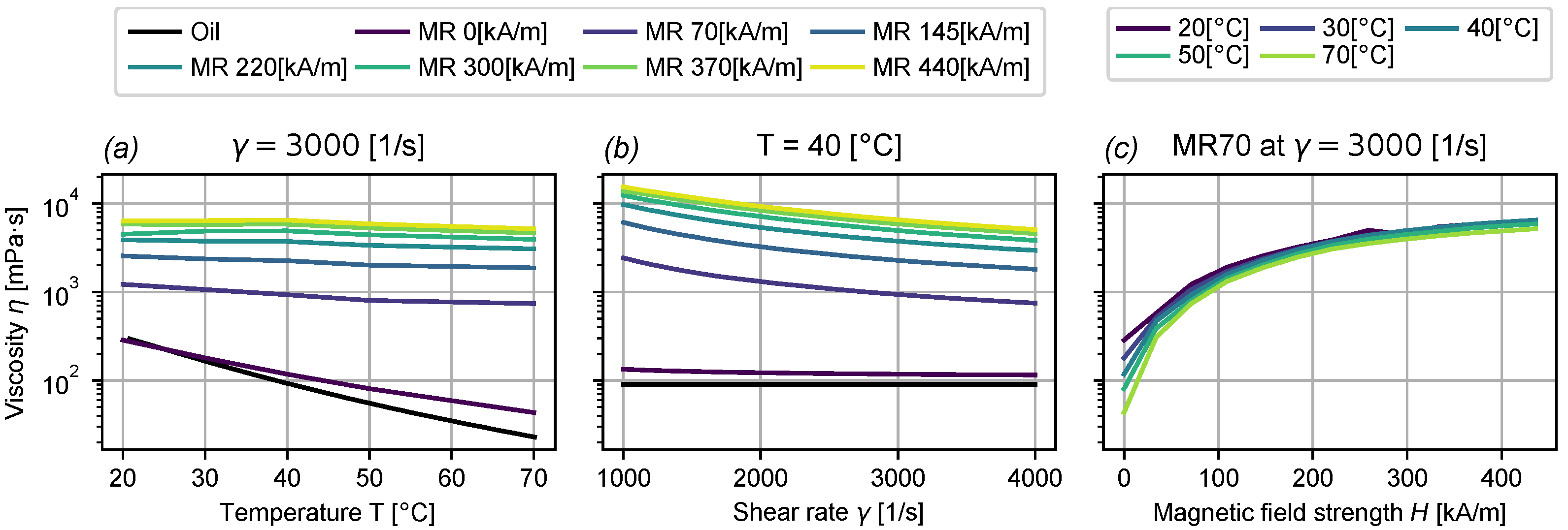
2.3. Lubricant Properties

Two different lubricants were tested for this study. A standard SAE 30 mineral oil, Castrol MHP 153, was used to obtain a reference measurement, while the MR measurements were performed with the MR fluid MRHCCS4-A containing 70% particles by weight [30]. From this point on, these lubricants will be referred to as ‘Oil’ and ‘MR 70%’ (or simply ‘MR’), respectively. An Anton Paar MRC 302 rheometer [31] with a cone-on-plate geometry was used to measure the viscosity of the two lubricants as a function of temperature, shear rate, and magnetic field strength (only for the MR fluid); the results are shown in Figure 3. The shear-thinning properties of the MR fluid are visible in Figure 3b, and all figures (Figure 3c in particular) show the increase in viscosity with increasing magnetic field strength. It can also be seen that the effect of very strong magnetic fields is relatively minor due to the effects of the magnetic saturation of the particles. Finally, Figure 3a shows that similar to oil, the MR fluid viscosity decreases with temperature, but interestingly, this decrease is stronger when no magnetic field is applied. The reduced influence of temperature on the viscosity when a magnetic field is present is the result of the influence of the particle structures, which are not influenced by temperature (below the Curie temperature) [4,32,33]. This means that the relative increase in viscosity due to the application of a magnetic field actually goes up when the temperature increases.

To be able to use these viscosity data in the numerical model (described in Section 2.4), a viscosity model can be fitted to the data. The Bingham plastic and Herschel–Bulkley models are frequently used for this purpose; both of these models use a yield stress to represent the very large increase in viscosity (almost a solidification) at shear stresses near zero. More important is that the Herschel–Bulkley model also incorporates shear thinning, which is generally considered to make it more accurate for use in high-shear-rate applications (such as journal bearings) [2,7]. The Herschel–Bulkley model is represented by Equation (1), where $|\overrightarrow{\tau }|$ and $|\overrightarrow{\dot{\gamma }}|$ are the shear stress and shear rate magnitudes, respectively, K is a proportionality constant called the consistency index, ${\tau }_y$ is the yield stress, and m is the flow index that determines whether the fluid is shear-thinning ($m<1$) or shear-thickening ($m>1$).

$$|\overrightarrow{\tau }|={\tau }_y+K{\left|\overrightarrow{\dot{\gamma }}\right|}^m$$

(1)

This equation can be rewritten to the form $|\overrightarrow{\tau }|=\eta |\overrightarrow{\dot{\gamma }}|$, and isolating the apparent viscosity $\eta$ then results in Equation (2), which can be fitted to the rheometer data. For this equation, it is assumed that the shear stress in the fluid is larger than the yield stress.

$$\eta ={\displaystyle \frac{{\tau }_y+K{\left|\overrightarrow{\dot{\gamma }}\right|}^m}{|\overrightarrow{\dot{\gamma }}|}}$$

(2)

However, in its current form, the Herschel–Bulkley model does not yet include the effects of variations in magnetic field strength H or temperature T. Starting with the former, only limited research could be found about magnetic field strength-dependent MR Herschel–Bulkley fits (or Bingham fits). One paper describes the use of an asymmetrical sigmoidal (‘S’-shaped) function to model the relation between yield stress and magnetic field strength, while keeping the other Herschel–Bulkley parameters constant [17]. Similar symmetric sigmoidal functions have also been used to describe the ‘S’ shape of a standard magnetisation (hysteresis) curve of a solid, where the initial linear relation between magnetisation and field strength tapers off once the material saturates [34,35]. Based on this information, it was found to be possible to fit the MR fluid viscosity data at a constant temperature by allowing all three Herschel–Bulkley parameters to depend on magnetic field strength with a symmetrical sigmoidal function. Specifically, the error function was used, resulting in Equation (3), where C is one of the three Herschel–Bulkley parameters (${\tau }_y$, m, or K), $c_1$ to $c_4$ are the fit constants, and H is the magnetic field strength in A m⁻¹.

$$C=c_{1}erf\left(c_2\left(H-c_3\right)\right)+c_4$$

(3)

With Equation (3), the Herschel–Bulkley model was fitted to the viscosity data from Figure 3 for a constant temperature of 36 °C (the assumed fluid film temperature in the bearing). Finally, including the effect of variations in temperature was achieved by simply multiplying the Herschel–Bulkley fit at 36 °C with a normalised exponential expression, resulting in Equation (4), where $\beta$ is the temperature–viscosity coefficient and T₀ = 36 °C. A similar viscosity–temperature dependence for MR fluids was found previously in the literature [33], although the slightly more complex Arrhenius equation was used in that case.

$$\eta ={\displaystyle \frac{{\tau }_y+K{\left|\overrightarrow{\dot{\gamma }}\right|}^m}{|\overrightarrow{\dot{\gamma }}|}}{e}^{\beta (T-T_0)}$$

(4)

The magnetic field strength–dependence of $\beta$ could be modelled with Equation (3) as well; the final values for all of the fit constants for ${\tau }_y$, m, K, and $\beta$ are shown in

Table 2. Coefficient values for the magnetic field strength-dependent Herschel–Bulkley viscosity fit of MRHCCS4-A.

C	Unit	${\mathit{c}}_1$	${\mathit{c}}_2$	${\mathit{c}}_3$	${\mathit{c}}_4$
${\tau }_y$	$\mathrm{Pa}$	6605	5.151 × 10−6	1.601 × 105	5013
K	Pa·sm	210.3	1.007 × 10−5	2.553 × 105	210.7
m	-	0.9614	1.039 × 10−5	1.570 × 105	1.992
$\beta$	°C−1	3.638 × 10−2	3.785 × 10−5	0	−4.260 × 10−2

. The viscosity model obtained with these values combines three basic relations for the rheology of an MR fluid, relating apparent viscosity to shear stress (Herschel–Bulkley), temperature (exponential fit), and magnetic field strength (symmetric sigmoidal). For engineering purposes, this basic combination was found to be sufficiently accurate: at a constant temperature of 36 °C with a varying shear rate and magnetic field strength, this fit has a normalised RMSE of 0.044; for temperatures of 20 °C and 70 °C, this changes to 0.0858 and 0.102, respectively. Keeping the magnetic field constant instead and fitting for varying shear rate and temperature results in a normalised RMSE of 0.0866 at 0 kA m⁻¹ and 0.0580 at 440 kA m⁻¹.

2.4. Numerical Model

The experimental measurements obtained with the setup were compared to a numerical model that was developed previously. This paper will only show the equations required to solve the numerical model; for the full derivation, the reader is referred to our previous paper [36]. The aim of the comparison in this paper was to verify the accuracy of the model when applied to MR fluids, and to check its usefulness for the optimisation of the magnetic field. This isothermal model is based on the laminar 2D Reynolds equation and incorporates cavitation, as well as the non-Newtonian characteristics of an MR fluid.

Starting with the Herschel–Bulkley model, the apparent viscosity is once again determined by rewriting Equation (1) using the form $|\overrightarrow{\tau }\left|=\eta \right|\overrightarrow{\dot{\gamma }}|$, but unlike Equation (2), where the viscosity is expressed as a function of the shear rate, Equation (5) shows the viscosity as a function of the shear stress.

$$\begin{array}{cc}\hfill \eta & ={\displaystyle \frac{K^{\frac{1}{m}}\left|\overrightarrow{\tau }\right|}{f{\left(|\overrightarrow{\tau }|-{\tau }_y\right)}^{\frac{1}{m}}}}\hfill \\ \hfill f& =\left\{\begin{array}{cc}{\displaystyle 1}\hfill & \mathrm{if}|\overrightarrow{\tau }|\ge {\tau }_y\hfill \\ {\displaystyle 0}\hfill & \mathrm{if}|\overrightarrow{\tau }|<{\tau }_y\hfill \end{array}\right.\hfill \end{array}$$

(5)

In order to use the Herschel–Bulkley model with the Reynolds equation, a modification is required to allow viscosity variations over the film thickness. To account for this, a generalised Reynolds equation has been derived following the method pioneered by Dowson [37], resulting in Equation (6). Here, $F_0$, $F_1$, and $F_2$ are flow factor integrals that depend on the apparent viscosity, ${\overrightarrow{u}}_b$ is the velocity of the shaft, and h is the film thickness given by Equation (7), with nominal film thickness $h_0$, eccentricity $\epsilon$, and attitude angle ${\varphi }_a$ (see Figure 4).

$$\begin{array}{}\hfill \overrightarrow{\nabla }\left(-h^3\left(F_2-{\displaystyle \frac{F_1^2}{F_0}}\right)\overrightarrow{\nabla }\xi +\psi h\left(1-{\displaystyle \frac{F_1}{F_0}}\right){\overrightarrow{u}}_b\right)=0\end{array}$$

(6)

$$h=h_0(1-\epsilon cos(\varphi -{\varphi }_a))$$

(7)

In this Reynolds equation, cavitation is included using mass-conserving JFO boundary conditions, which are implemented by replacing both the pressure p and lubricant fraction $\psi$ with functions of a new variable $\xi$ (see Equations (8) and (9)) [38]. In assuming that every point in the bearing is either part of a full film region ($p>0$, $\psi =1$) or a cavitated region ($p=0$, $0\le \psi <1$), the generalised Reynolds equation can be solved for $\xi$, with the positive part representing the pressure, and the negative part representing the mass fraction.

$$\begin{array}{cc}\hfill & \begin{array}{}\hfill p=(\xi \ge 0)\xi \end{array}\hfill \end{array}$$

(8)

$$\begin{array}{cc}\hfill & \begin{array}{}\hfill \psi =1+(\xi <0)c_f\xi \end{array}\hfill \end{array}$$

(9)

Numerical stabilisation is required to prevent oscillations in the convection-dominated cavitation region. In this case, artificial diffusion was implemented, which is controlled by the variable $c_f$ in Equation (9). It is possible to calculate the minimum value of $c_f$ that will still prevent oscillations [36,38], which results in Equation (10), where $h_e$ is the local mesh size.

$$c_f=\left(F_2-{\displaystyle \frac{F_1^2}{F_0}}\right){\displaystyle \frac{h^2}{h_e\left(1-\frac{F_1}{F_0}\right){\overrightarrow{u}}_b}}$$

(10)

The flow factors that appear in the Reynolds equation are calculated with Equation (11), where the inverse of the viscosity is integrated over the film thickness coordinate z. As can be seen in Equation (5) for the viscosity, this requires a formula for the shear stress $\overrightarrow{\tau }$ as a function of z, which is provided by Equation (12).

$$F_n={\int }_0^h{\displaystyle \frac{z^n}{\eta }}\mathrm{d}z$$

(11)

$$\overrightarrow{\tau }=\left(z-{\displaystyle \frac{F_1}{F_0}}\right)\overrightarrow{\nabla }p+{\displaystyle \frac{{\overrightarrow{u}}_b}{F_0}}$$

(12)

Finally, a solution to the numerical model is obtained by solving the Reynolds equation (Equation (6)) for $\xi$, Equation (11) for the flow factors $F_0$, $F_1$, and $F_2$, and the horizontal and vertical load balances $F_x$ and $F_y$ for the shaft attitude angle ${\varphi }_a$ and eccentricity $\epsilon$, respectively (Equations (13) and (14)).

$$F_x={\int \int }_{S}psin\varphi \mathrm{d}A=0$$

(13)

$$F_y={\int \int }_{S}pcos\varphi \mathrm{d}A-W_a=0$$

(14)

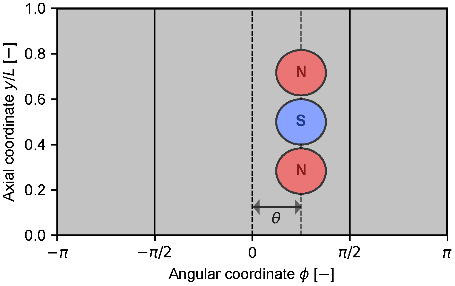
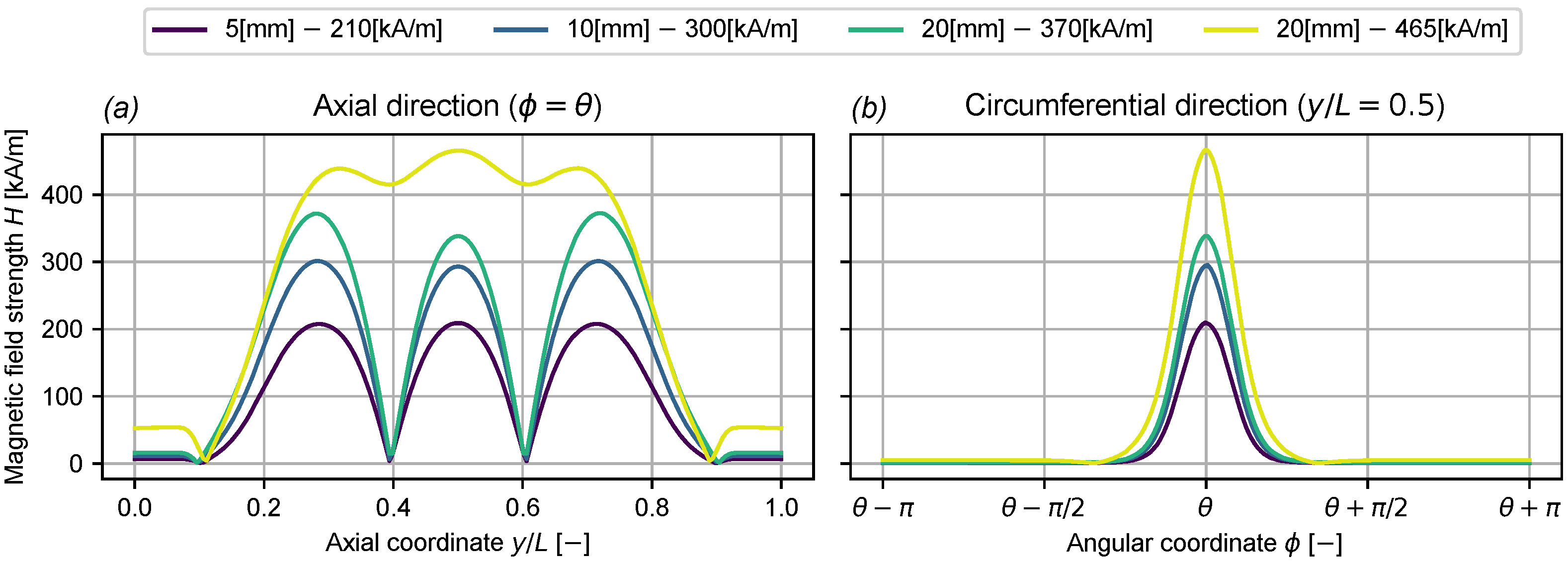
2.4.1. Magnetic Field Calculation

The final requirement for solving the numerical model is the magnetic field in the film, which will be determined numerically. For this paper, the magnetic field that was used in the experiments was generated by three neodymium permanent magnets placed side-by-side in the axial direction, as shown in Figure 2. During these experiments, the strength of the magnets was varied (by changing their length, denoted by dimension L3) as well as their angular position (in the $\varphi$-direction). Figure 5 shows the 2D computational domain of the Reynolds simulation, where the angular position of the magnets is indicated with the angle $\theta$. Note that the polarity of the magnets was alternated in an attempt to reduce the magnetic field strength in the film outside the area covered by the magnets. This was done in an attempt to reduce the friction increase, since the magnetic field simulations indicated that with opposing polarities, the strength of the field far away from the magnets would be much lower (relative to the strength close to the magnets) compared to having the same polarities. The aim was to use this to focus the viscosity increase on the area of the film directly below the magnets, while limiting the viscosity increase far away, thereby limiting the increase in friction. One experiment was also performed where the polarisation of the magnets was not alternated, to maximise the magnetic field in the film.

For the purposes of the magnetic field simulation, only the magnets themselves, the housing, and the shaft are considered. Both the inner and outer bearing bush are non-magnetic, and the influence of magnetisable components outside the bearing housing was found to be negligible. Furthermore, small features in the geometry of the housing (internal channels, bolt holes, bolts, etc.) are removed to reduce complexity, meaning that the final bearing housing geometry is axisymmetric in the simulation. As a result, the magnetic field in the film is only calculated for different magnet sizes at $\theta =0$. For other angles $\theta$, that magnetic field solution is simply shifted in the $\varphi$-direction by $\theta$ radians.

The resulting 3D magnetic field simulation was implemented in the FEM software package COMSOL Multiphysics^® 6.1 [39] with the standard ‘Magnetic Fields, No Currents (mfnc)’ interface. This simulation is almost identical to the one performed in our previous work. For details about the implementation in COMSOL or the computational geometry, the reader is referred to that work [27]. The only difference with that study is the variation in the length of the magnets. The resulting magnetic fields in the fluid film are shown in Figure 6 as a function of this length and for a constant magnet angle of $\theta$ radians. The strongest magnetic field in this figure, with a peak strength of 465 kA/m⁻¹ is the field that was created by placing all three magnets in the same polarity direction (switching the polarity of the central magnet from S to N; see Figure 5). This is the reason why the magnetic field strength does not go to zero in between the magnets, in contrast to the other magnetic fields. For simplicity, the magnetic fields will be referred to by their peak field strength values from now on.

2.4.2. Software Implementation

The full numerical model was solved with the FEM software package COMSOL Multiphysics^® 6.1 [39]. The Reynolds equation and flow factors (Equations (6) and (11)) were implemented as General From PDE’s with quadratic Lagrangian shape functions, while the load balances (Equations (13) and (14)) were implemented as global equations. Note that the flow factor integrals were evaluated with COMSOL’s numerical integration routine integrate. The 2D computational domain on which the equations were solved was meshed with a structured quadrilateral mesh with 10,000 (100 × 100) elements, for a total of 311,010 degrees of freedom. The domain is shown in Figure 5. A periodic boundary condition was used to connect the solution at $\varphi =-\pi$ and $\varphi =\pi$ (Equation (15)), while Dirichlet boundary conditions setting $\xi =0$ were placed on both the inlets at $\varphi =-\pi /2$ and $\varphi =\pi /2$ and outlets at $y=0$ and $y=1$ (Equation (16)). A constant pressure boundary condition was chosen for the inlets, because while the lubricant was being pumped at a constant volume pump, the inlet grooves extend along the entire length of the bearing and connect directly to both outlets. For this reason, it is expected that the bearing will only take as much lubricant from the inlet flow as it needs, while the rest of the inflowing lubricant flows directly to the outlets through the inlet grooves.

$$\begin{array}{cc}\hfill & {\xi }_{\varphi =-{\displaystyle \frac{\pi }{2}}}={\xi }_{\varphi ={\displaystyle \frac{\pi }{2}}}\hfill \end{array}$$

(15)

$$\begin{array}{cc}\hfill & \xi =0\mathrm{at}y=0,y=1,\varphi =-{\displaystyle \frac{\pi }{2}},\varphi ={\displaystyle \frac{\pi }{2}}\hfill \end{array}$$

(16)

The problem is solved with the standard COMSOL Newton–Raphson solver with under-relaxation; convergence is assumed when the relative tolerance on the solution is lower than 1 × 10⁻³. The model has been validated for a relative tolerance of 1 × 10⁻⁶ (see also [36]); as an indication, the difference with a tolerance of 1 × 10⁻³ is on average about 0.1% for the film thickness. The solver uses three steps: the first step solves only the Reynolds equation, the second steps solves the Reynolds equation and flow factors, and the final step solves the Reynolds equation, flow factors, and load balances. The solver was modified slightly for the final step, where the relaxation factor was set to a constant value of 0.2; for the other steps, this factor was chosen automatically.

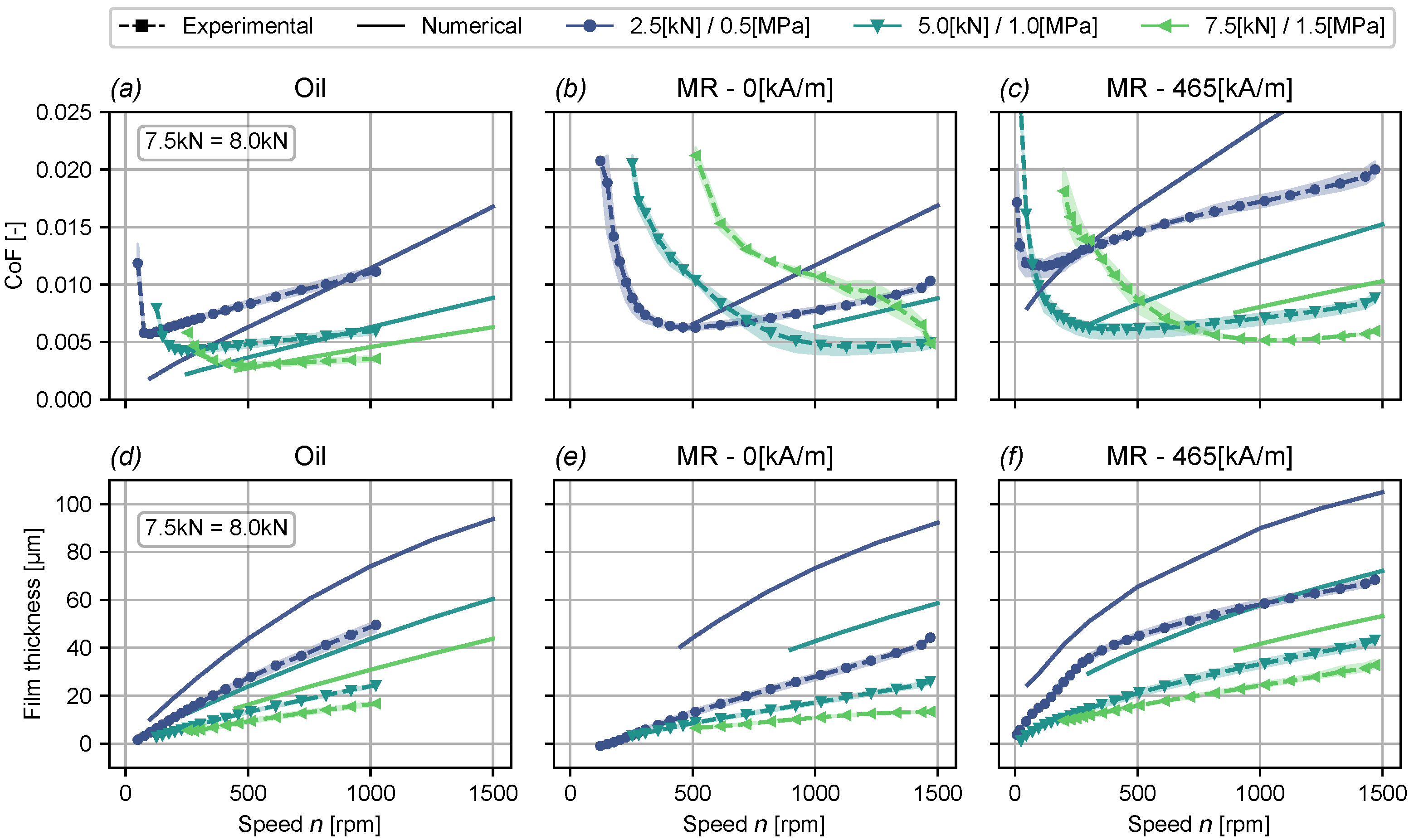
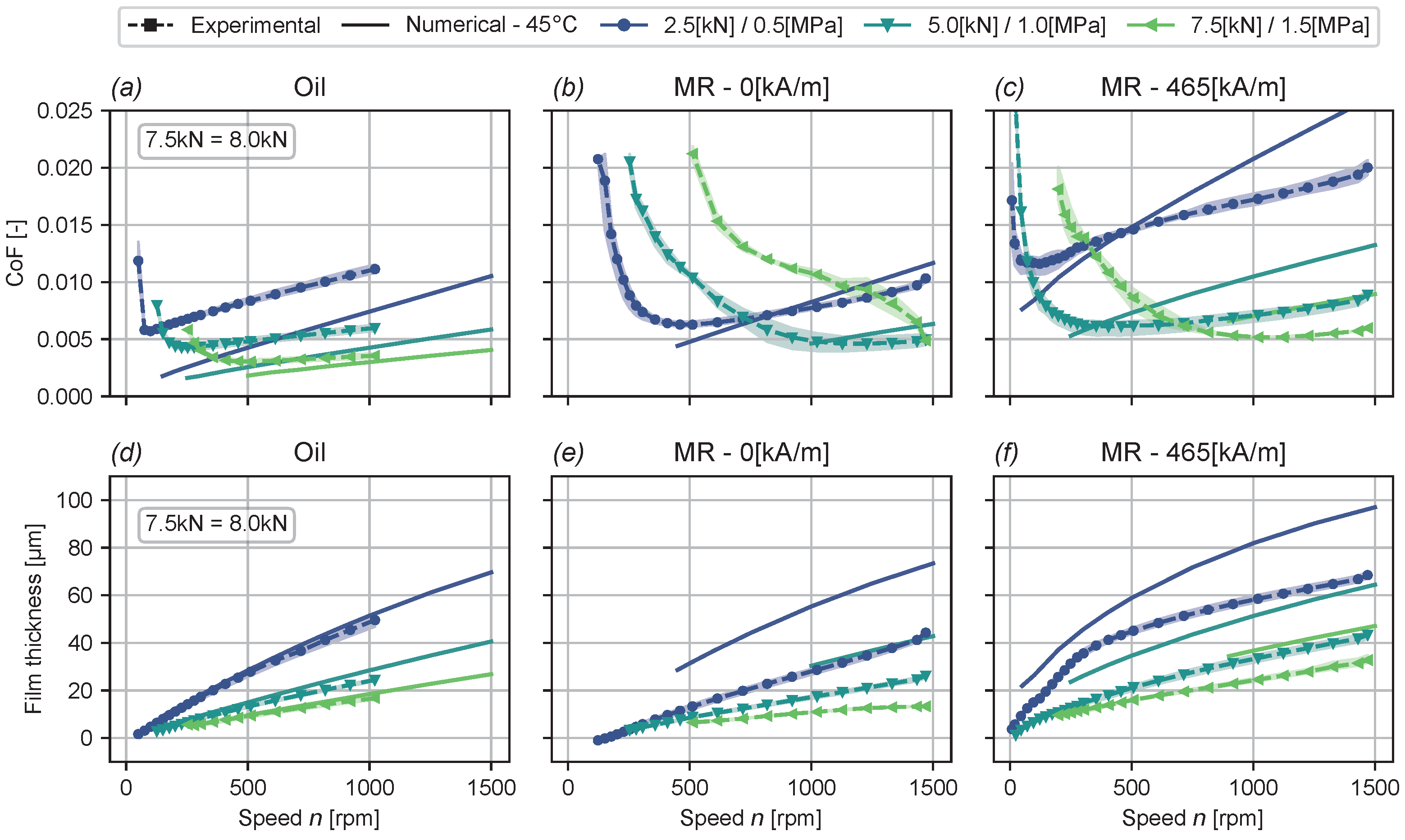
3. Results and Discussion

This section presents the results of the experimental and numerical work that was performed, and is divided into three subsections. The first subsection describes an initial optimisation of the angle of the magnets with the numerical model, and shows the experimental verification. In the second subsection, this optimised angle is used while varying the magnetic field strength and the applied load. This was carried out both experimentally and numerically, and the results are compared with those of the reference lubricating oil. The final subsection discusses the deviations between the numerical model and the experiments.

3.1. Magnet Angle Optimisation

It was decided to start the investigation using the model to optimise the angle $\theta$ of the permanent magnets (see Figure 5), and to use the experimental setup to verify these results. The goal of this optimisation was to find the angle where the localised increase in film viscosity due to the magnetic field would result in the largest increase in film thickness (or equivalently, the largest decrease in eccentricity). Since the optimal angle was found to vary with speed, the optimisation was performed for a constant (low) speed of 200 rpm; at this speed, the bearing was experimentally found to be in mixed or boundary lubrication without the presence of a magnetic field. The reason for optimising at low speed, instead of at high speed, is that in most situations, the film of a bearing would already be sufficiently thick at high speeds. Increasing the viscosity would make it even thicker, but would mostly just reduce efficiency since it also increases friction. Optimising the magnetic field to increase film thickness at low speeds is expected to be more useful, since this reduces the transition speed, meaning the minimum speed with the bearing is still in the hydrodynamic regime. It would have been more effective to optimise the transition speed directly, and for an oil-lubricated, bearing this could be realized by checking when the minimum film thickness becomes smaller than the combined roughness of the shaft and bearing [40]. With an MR-lubricated bearing, this is not possible due to the presence of microparticles in the minimum film, which are expected to have a large influence on the low-speed hydrodynamic performance of the bearing (as will be discussed at the end of Section 3.2.1). For that reason, the model is only valid in the hydrodynamic regime.

Figure 7a shows the results of the numerical optimisation, with film thickness plotted as a function of the angle of the magnets, as well as the experimental verification that was performed afterwards for a select number of magnet angles. Note that the verification could not be performed for magnet angles lower than -45°, since that would cause the support bracket holding the magnets to collide with one of the inlets. Figure 7b shows the corresponding numerically calculated pressure profiles at the centreline of the bearing. When examining the results, it can be seen that both the experimental and numerical results indicate the existence of an optimal angle that maximises the film thickness at the minimum film. Specifically, the optimisation predicts an optimum around −42° with a film thickness of 37.6 μm, whereas the experiments show the optimum to lie around −22.5° with a film thickness of 18.4 μm.

Counter to the initial expectations of the authors, both the model and experiments show that the optimum lies quite far upstream from the minimum film (which the experiments indicate lies between $20<\varphi <40$ for 200 rpm, depending on the exact value of $\theta$), and that placing magnets near or just after minimum film does not result in a higher pressure peak. Instead, placing the magnets farther upstream from the minimum film results in a lower but also wider pressure peak, with an overall higher load capacity. Placing the magnets too far upstream will reduce the load capacity again, since the pressure profile will be so wide that a substantial part will act mostly in the horizontal direction.

It seems intuitive to think that this might in some way be related to the strong shear-thinning characteristics of the MR fluid. The shear rate will be relatively high near the minimum film, and the effect of the magnetic field on the viscosity will therefore be smaller than in regions of the film with lower shear rates. However, rerunning the simulation while assuming a constant shear rate for the purposes of calculating the viscosity (meaning that the fluid is no longer shear-thinning and that its viscosity depends only on the magnetic field strength) gives qualitatively similar results. It therefore seems that the optimum may actually be caused by the geometry of a journal bearing, not by the shear-thinning rheology of the MR fluid.

3.2. Varying Magnetic Field Strength and Load

In this section, experimental and numerical Stribeck curves are shown for the MR-lubricated bearing, first with a varying magnetic field strength and then with a varying load applied. These results will be shown alongside the results for oil lubrication, to see how MR lubrication compares with a more traditional lubricant. During the MR measurements, the angle of the magnets was set to the optimal value (for the specific magnetic field used in this research) of θ = 22.5° identified experimentally in the previous section. It is worth mentioning that the model predicts that the optimal angle is dependent on the magnetic field strength; however, in this research, the angle was kept constant for all measurements. The reason for this is that the goal of these experiments was to show the effects of magnetic field strength and load in isolation, not to find the most optimal configuration for this specific bearing.

3.2.1. Magnetic Field Strength Variation

Figure 8a,b present experimental and numerical Stribeck curves for the MR-lubricated bearing as a function of magnetic field strength (with the magnets positioned as in Figure 5 at θ = −22.5°) for a constant load of 2.5 kN/0.5 MPa. Figure 8c,d present the corresponding film thickness plots, and all figures also show the curves for the bearing lubricated with the reference oil. For the experimental results, the dashed lines represent the average of the three repetitions of every measurement, and the shaded areas represent the maximum and minimum friction or film thickness values recorded during those three tests. The differences between the experimental and numerical results are obviously large, especially for the film thickness, but this will be discussed further in Section 3.3 as was mentioned before.

Both the experimental and numerical results do very clearly illustrate the effect that a magnetic field has on the viscosity of an MR lubricant. Increasing the strength of the magnetic field causes the lubricant viscosity to go up at the location of the magnets, which in turn causes thicker films and an associated reduction in the transition speed (defined as the speed where the friction coefficient has a minimum), but also an increase in the level of friction in the bearing. Furthermore, the results show that seemingly minor changes in the exact distribution of the field throughout the film can have large effects on the overall behaviour of the system. This can be seen by comparing the (experimental) Stribeck and film thickness curves for the field with peak a strength of 465 kA m⁻¹ and the curves with the lower peak field strengths. As an example, both the 370 and 465 kA m⁻¹ fields were created with three 20 × 20 mm cylindrical magnets placed in a line in the axial direction, but where the 465 kA m⁻¹ field was generated by having the polarity of all three magnets in the same direction, the weaker field was generated with the central magnet rotated to have its polarity opposite to its neighbours’. As discussed in Section 2.4.1, this polarity change was implemented in an attempt to reduce the friction increase by focusing the magnetic field (and therefore the viscosity increase) on the area of the film directly beneath the magnets. As a side effect, the peak magnetic field strength was reduced and the shape of the magnetic field beneath the magnets was changed as well (see Figure 6). One of these changes did seem to have the desired effect, at least at high speed, since at 1000 rpm, the film thickness with the 465 kA m⁻¹ field is around 18% higher than with the 370 kA m⁻¹ field, while the friction is more than 50% higher. However, at lower speeds, the effects of these changes are different, and the 87% increase in film thickness is accompanied by an increase in friction of only 65%. This shows that it is very important to accurately determine exactly which parts of the film should be magnetised when designing an MR-lubricated bearing.

The friction and film thickness curves for the same bearing lubricated with the reference oil are shown in Figure 8 as well. When comparing these curves with the ones for MR lubrication, it is interesting to notice that the MR-lubricated bearing can achieve either lower hydrodynamic friction and a higher transition speed (without a magnetic field), or a lower transition speed and higher hydrodynamic friction (with the 465 kA m⁻¹ field), but not both lower friction and a lower transition speed. Things become especially peculiar when looking at the curves of the bearing magnetised with the 300 kA m⁻¹ magnetic field. Even though the hydrodynamic friction coefficient is almost exactly the same as with oil lubrication, the transition speed is still more than 100 rpm higher. In spite of that, the film thickness plot shows that the film thickness of the MR-lubricated bearing at its transition speed is actually slightly higher than that of the oil-lubricated bearing. Furthermore, the transition from hydrodynamic to mixed or boundary lubrication occurs relatively suddenly with oil lubrication, with a sharp increase in friction once the shaft touches the bearing surface. With MR lubrication, on the other hand, this transition is much more gradual and there almost appears to be a transition region instead of a discrete, well-defined transition speed. It is hypothesised that all of these effects are related, and are caused by the presence of the large concentration of particles in the MR fluid (70% by mass or around 20% by volume).

At high speeds, the particles will be in suspension, but when the speed is lowered and the shaft starts approaching the bearing surface, it may be assumed that particles will be trapped between the two surfaces. Because there are so many particles, this could result in a layer that is multiple particles thick; with the shaft sinking further and further into this layer, the lower the speed becomes. The gradual increase in the compressive forces would then correspond to the gradual transition increase in friction observed during the experiments. However, while wear tests using MR lubricant have shown that particles are present in the contact zone during boundary lubrication [41,42], the behaviour of the particles during very-low-speed hydrodynamic lubrication is not known in the literature. This will require further research.

3.2.2. Load Variation

Figure 9a–c show the experimental and numerical Stribeck curves for oil and MR lubrication at three different loads, with Figure 9c,d showing the corresponding film thicknesses. To illustrate the effect of the magnetic field under increasing load, the MR fluid was tested both without a magnetic field, and with the strongest magnetic field with a peak strength of H = 465 kA m⁻¹.

Starting with the standard lubricating oil, the Stribeck curves and film thickness plots (Figure 9a,c) show that the bearing exhibits the expected behaviour, with a higher load leading to a lower friction coefficient, a smaller film thickness, and a lower transition speed. Other than the transition speed, these trends were also captured by the hydrodynamic numerical model, although the absolute values clearly deviate, as was already observed in the previous section. In comparing these curves with those of the unmagnetised (Figure 9b,d) and magnetised (Figure 9c,e), the MR-lubricated bearing does not immediately show any qualitative differences. It should be noted that all MR fluid measurements were performed with a higher starting speed of 1500 rpm, the maximum speed of the motor. This was necessary for the measurements with unmagnetised MR lubricant loaded to 5.0 KN and 7.5 KN. Due to the low viscosity of the unmagnetised MR lubricant, the bearing never reached hydrodynamic lubrication when starting at 1000 rpm with these loads, and even 1500 rpm was not high enough with a load of 7.5 KN. Applying the magnetic field solved this issue by reducing the transition speed to around 1000 rpm for this load, demonstrating once again the large effect of the magnetic field on the MR lubricant viscosity.

However, there does appear to be a difference in the way that the performance of the oil- and MR-lubricated bearings scales with the applied load. This is especially obvious when comparing the transition speeds. At the lowest load, the transition speed of the MR-lubricated bearing goes from around 500 rpm without a magnetic field to around 75 rpm with a magnetic field, which is actually slightly lower than the 100 rpm transition speed of the oil-lubricated bearing. In contrast, at the highest load, the transition speed is only around 1000 rpm with magnetised MR lubrication, compared to around 500 rpm with oil. The medium load of 5 KN falls in between these two extremes.

The reason for this difference in scaling can be likely attributed to the shear-thinning characteristics of the MR fluid. Higher loads will lead to higher film pressures, and therefore to higher shear rates, particularly in the converging section of the film where the pressures are large. Higher shear rates will reduce both the viscosity itself and the increase in viscosity due to the application of a magnetic field (see Figure 3b). At a higher load, the bearing will therefore experience (relative to the lower load) a smaller increase in film thickness and friction, meaning also a smaller reduction in the transition speed, which is exactly what was observed experimentally. Some of this could likely be mitigated by magnetising a larger amount of fluid in the film, for example, by adding additional rows of permanent magnets parallel to the single row used in the experiments (see Figure 5). This would increase the amount of magnetised, high-viscosity lubricant, thereby increasing the pressure generation. Similarly, stronger magnetic fields could be used, although it should be taken into account that the particles in the fluid will saturate at some point. All in all, it seems that the shear-thinning properties of the MR lubricant used in this research may necessitate these additional measures when the load on the bearing increases, which is obviously not the case with standard Newtonian lubricating oils.

3.3. Discussion on the Numerical Model

As was remarked in the previous sections, there are clear and large deviations between the experimental and numerical results presented in Figure 7, Figure 8 and Figure 9, both for the friction coefficient and for the film thickness. Though the general trends in friction and film thickness are similar for both the experimental and numerical results, the quantitative differences are large enough to require additional investigation. Three main ways have been identified in which the numerical results differ from the experiments, these will be referred to as points 1, 2, and 3 hereafter:

• The model overpredicts both the friction coefficient and the film thickness for all operating conditions, independent of the type of lubricant.
• The model underpredicts the increase in film thickness due to an increase in magnetic field strength with the MR-lubricated bearing (Figure 9e,f).
• The model does not predict any differences between oil and unmagnetised MR lubrication, even though the experimental results clearly show that such a difference exists (Figure 9d,e).

To explain these differences, an extensive investigation was conducted into phenomena that were not included in the initial model but could feasibly affect the experimental results. This included effects such as the elastic deformation of the steel and polymer bearing sleeves and of the steel housing, actuator, and bearing housing misalignment, wear or running-in of the polymer bearing sleeve, and the exact inlet boundary conditions used in the model. For the specific setup in this study, all of these effects were found to have negligible influence on the film thickness and friction of the bearing. The rest of the section will discuss the remaining phenomena that were expected to play a larger role in the experiments.

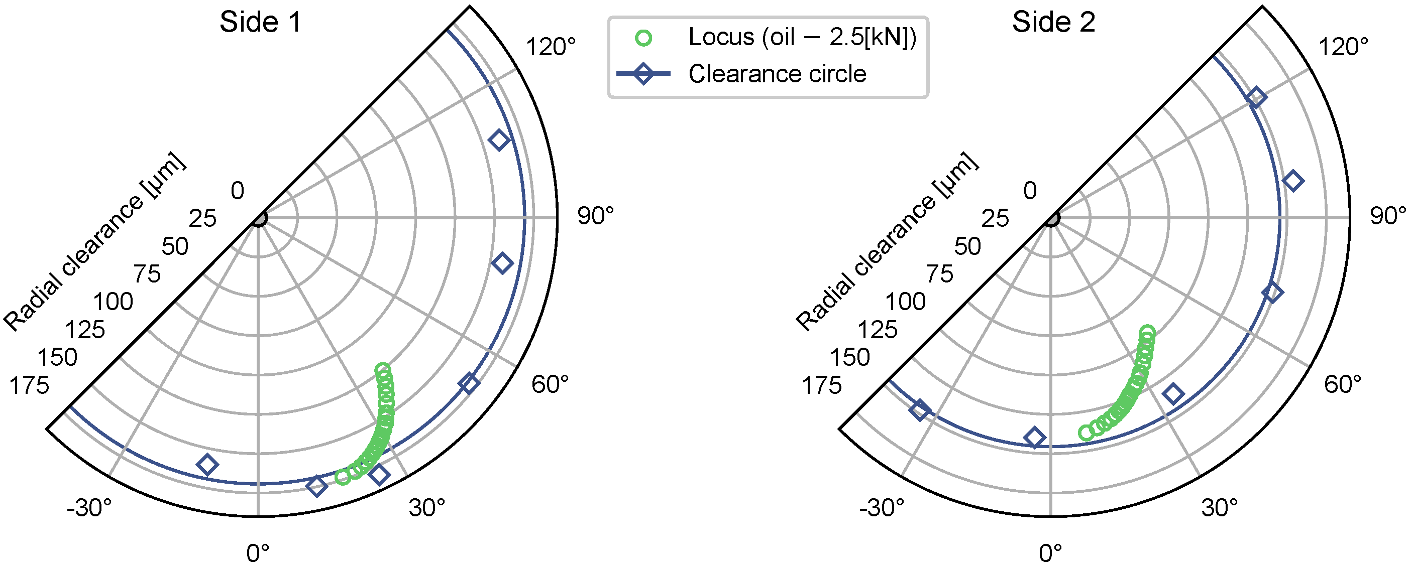
3.3.1. Bearing Sleeve Shape Errors

The first phenomenon that was expected to affect the performance of the bearing is related to the bearing geometry. As was mentioned in Section 2, the film thickness in the bearing is determined as a function of shaft speed by averaging the film thickness measured on both sides of the bearing with two sets of two capacitive distance sensors mounted 90° apart. These sensors were calibrated by measuring the clearance circles of the bearing, which were effectively constructed by loading the bearing at zero speed such that the eccentricity of the shaft was set to $\epsilon =1$. The capacitive sensors were read out in this position, and this process was then repeated for a number of attitude angles $0\le {\varphi }_a\le 2\pi$ (12 positions were used in this study). The resulting measurements form collections of points through which the clearance circles can be fitted, which will always bound the shaft locus measurements for non-zero speeds since $\epsilon \le 1$ in that case. Figure 10 shows a representative example of the loci and (one half of) the clearance circles measured on both sides of the bearing; examining the differences between side 1 and 2 immediately reveals two issues. First of all, the radial clearance on side 1 is 25 μm larger than on side 2 (170 μm vs. 145 μm), which means the bearing is tapered. This was also verified with a three-point micrometer. Second, the collections of data points forming the clearance circles do not lie perfectly on the fitted circles; the fits have standard deviations of 9.0 and 6.0 μm for sides 1 and 2, respectively, indicating cylindricity errors. Specifically, on side 1, the data points indicate the presence of a shallow groove between roughly 10 and 30°, with the locus showing that the shaft gets stuck in this groove at low speeds. On side 2, this groove is not present; the radial clearance in that location is instead smaller than predicted by the fitted circle, causing the shaft locus to move toward the 0° position as expected. Due to these shape errors, and due to the differences in shape between the two sides, the shaft and bearing are forced into a mostly horizontal misalignment at low speeds, with an 8.5° difference in attitude angle at the lowest speed. Compare this to the highest speed, where the attitude angles are effectively the same on both sides. In contrast, the amount of vertical misalignment seems minimal since the eccentricities on both sides are fairly similar at the lowest speeds; on both sides, the loci approach the actual clearance circles implied by the data points when the speed is lowered. The lack of vertical misalignment in spite of the taper of the bearing means that the bearing has rotated such that it is parallel to the shaft around the minimum film, possibly because the load is applied to hydrodynamic bearing housing through a hydrostatic bearing, which is not perfectly stiff against rotations.

The reasons for the existence of these shape errors is not known exactly, but similar issues have been observed before with polymer bearings for water lubrication [40]. Possible causes of the shape errors were stated to be machining or assembly errors, water soaking, thermal expansion, and/or progressive wear. Since the shape errors of the bearing in the current paper were already present before the start of the first measurement, machining or assembly errors seem the most likely.

The exact influence of these shape errors on the film thickness and friction coefficient in the model is difficult to determine without accurately measuring the entire geometry of the bearing sleeve, which is not a trivial task. However, it is known that shape errors can have a large (negative) effect on the film thickness of a journal bearing [43], which means it is feasible that these errors are at least part of the reason for the poor predictions of the model (specifically points 1 and 2 at the start of Section 3.3). It is also feasible that the misalignment of the shaft at low speed affected the optimal position of the magnets (see Figure 7), possibly explaining why the predicted optimum differed from the measured one. For these reasons, it is recommended that future research using polymer bearings for MR lubrication focuses on the careful machining and verification of the bearing shape, to minimise any errors in the geometry.

3.3.2. Film Temperature

Another likely reason for some of the differences between the model and experiments relates to the temperature of the fluid film in the bearing. Based on the measurements of the thermocouples in the sleeve and in the outlet flow, the fluid film was assumed to be isothermal at 36 °C for the purposes of the model. However, these thermocouple measurements are likely poor indicators of the actual film temperature. The reason for this is that thermocouples T0 through T2 in the sleeve (see Figure 2 for their placement) only measure the temperature of the outer steel sleeve used to reinforce the inner polymer bearing bush. This was realised to make manufacturing and assembly easier, but since polymers conduct heat poorly the thermocouples are separated from the fluid film by 4 mm of what is effectively an insulator. After this was realised, thermocouples T3 and T4 were placed in the outlet flow in an attempt to obtain a better estimate. While the temperatures reported by these thermocouples were 1 to 2 degrees higher, these results were found to be poor indicators as well due to the design of the lubrication grooves. To simplify manufacturing, these grooves span the entire axial length of the bearing, meaning that part of the 0.3 L min⁻¹ inlet flow of cold 32 °C lubricant will flow directly to the outlets. T3 and T4 therefore measure the temperature of a mixture of hot and cold lubricant, and cannot be used as an indication of the film temperature either.

All in all, it can be concluded that the thermocouples used in the setup underestimate the actual film temperature. Since higher film temperatures will result in lower friction and film thickness, this issue could address point 1 in Section 3.3. To investigate this a bit more, Figure 11 shows the experimental results for varying bearing load from Figure 9, with updated model results for a constant temperature of 45 °C. At this film temperature, the model was found to fit the experimental film thickness results for oil lubrication very well (Figure 11d), and predicts very similar slopes for the friction coefficients (Figure 11a). A film temperature of around 45 °C does not seem unreasonable based on the 36 °C measured at the thermocouples, especially when considering that the film temperature could also be lower when the effects of the shape errors discussed in the previous section are taken into account.

The model results for MR lubrication at 45 °C fit the experiments less well, especially for the film thickness, even though there are improvements. Specifically, the increase in film thickness due to the application of the magnetic field (point 2 at the start of Section 3.3) matches the experimental results more closely at higher temperatures. For example, at 1500 rpm, the increase in film thickness changes from 12.8 to 23.5 μm when the temperature goes from 36 to 45 °C, with the experiments showing a 24.3 μm increase. The reason for this is the dependence of the temperature–viscosity coefficient $\beta$ on the magnetic field, with $\beta$ rapidly becoming smaller with increasing field strength H (see Section 2.3 and Figure 3).

The absolute difference in film thickness is still large for the MR-lubricated bearing at 45 °C. In fact, the isothermal temperature of the film would have to be 60 °C for the unmagnetised bearing and 80 °C for the magnetised bearing to have the model match the experiments. While it is to be expected that the magnetised bearing would have a higher film temperature due to the increased viscosity, these temperatures seem unrealistic considering the thermocouple measurements (despite their flaws). For the MR-lubricated bearings, temperature is therefore probably not the only effect with a significant influence on bearing performance.

Finally, it should be noted that the film temperature will not be isothermal in reality, which is something that can also affect the model results. With the model used in this research, determining the full 3D temperature profile inside the film requires solving an energy equation for the temperature in addition to the generalised Reynolds equation, which is solved for the pressure, as realized previously in the literature [44]. The relation between viscosity and temperature is already defined by Equation (4), meaning that the main difficulty lies with applying proper boundary conditions. For example, thermal conduction in the shaft would probably have to be taken into account, as well as the temperature distribution in the lubrication grooves.

3.3.3. MR Fluids at Very High Shear Rates

The final effect that could explain some of the differences between the model and the experiments is the behaviour of the MR fluid at very high shear rates. MR fluids are generally used in damping or braking systems where the shear rates are relatively low, and because of this, commercially available rheometers for MR fluids focus on this low shear regime as well. For example, the cone-on-plate rheometer that was used for this study is only capable of measuring shear rates up to 4000 s⁻¹ at higher shear rates, the fluid will be flung out of the gap due to the centrifugal forces. However, the numerical model shows that the shear rates in the film of the journal bearing setup are expected to have orders of magnitude of around 1 × 10⁴ to 1 × 10⁵ s⁻¹ (depending on the operating conditions), much larger than the shear rates that can be attained with any of the commercial magnetorheometers (which should be capable of both temperature and magnetic field control). The only high-shear-rate (up to 4 × 10⁴ s⁻¹ viscosity measurements that could be found in the literature were realised with custom-built magnetorheometers and different MR fluids [45,46,47].

In this study, the high-shear viscosity data required for the model were instead obtained by extrapolating the low-shear rheometer data with the Herschel–Bulkely viscosity model (see Equation (5)). While the literature on custom high-shear magnetorheometers found that this model can fit high-shear-rate MR viscosity curves quite well, this does not change the fact that the viscosity is still extrapolated over 1 to 2 orders of shear rate magnitude in our case. It is possible that errors resulting from this extrapolation could explain the differences between the model predictions for MR and oil lubrication as described by point 3 in Section 3.3, since this issue does not affect the viscosity measurements of the Newtonian reference oil. However, this is impossible to find out without actually testing the MR fluid at these high shear rates using an appropriate (custom-built) magnetorheometer.

4. Conclusions

In the current research, the Stribeck curves and film thickness plots of a hydrodynamic journal bearing were compared experimentally and numerically for oil and MR fluid lubrication, under different loads and for different magnetic field strengths. Since the MR fluid used in this research had a lower viscosity than the oil when not magnetised, it was found experimentally that MR lubrication without a magnetic field resulted in thinner films and a higher transition speed, but also in lower hydrodynamic friction. On the other hand, a strong magnetic field caused a large increase in film viscosity and resulted in the thick films and low transition speeds frequently reported in the literature, as well as the associated friction increase. Interestingly, it was not possible to obtain both a lower transition speed and lower high-speed hydrodynamic friction with the MR lubricant compared to standard oil lubrication, irrespective of the magnetic field strength. This could be a negative influence of the presence of the MR particles in the minimum film during low-speed hydrodynamic lubrication. Finally, increasing the bearing load was found to lead to a reduction in the effect of the magnetic field on film thickness, transition speed, and friction coefficient, most likely because of the shear-thinning characteristics of the MR fluid combined with the higher shear rates due to the increased film pressures.

Designing a model to accurately capture all of these effects turned out to be difficult, with large deviations between the model predictions and the experimental findings. Part of this is probably related to the complex and only partially known rheology of an MR fluid, with a viscosity that depends on shear rate, magnetic field strength, and temperature. In this study, a basic relation was constructed for the apparent viscosity based on rheometer viscosity data as a function of these three parameters, showing this complexity. The other part of the deviations was likely caused by geometry errors in the polymer bearing used in the experiments. A polymer bearing was chosen for its wear properties under MR lubrication, but it has been found in the literature that polymer bearings are more difficult to work with than traditional metal bearings, sometimes resulting in shape errors similar to those observed in the bearing used in this research. For this reason, it is recommended that future research using MR-lubricated polymer bearings focuses on preventing geometry errors during the fabrication process.

References

1. Bossis, G.; Volkova, O.; Lacis, S.; Meunier, A. Magnetorheology: Fluids, Structures and Rheology. In Ferrofluids: Magnetically Controllable Fluids and Their Applications; Odenbach, S., Ed.; Springer: Berlin/Heidelberg, Germany, 2002; pp. 202–230. [Google Scholar] [CrossRef]
2. de Vicente, J.; Klingenberg, D.J.; Hidalgo-Alvarez, R. Magnetorheological fluids: A review. Soft Matter 2011, 7, 3701–3710. [Google Scholar] [CrossRef]
3. Ahamed, R.; Choi, S.B.; Ferdaus, M.M. A state of art on magneto-rheological materials and their potential applications. J. Intell. Mater. Syst. Struct. 2018, 29, 2051–2095. [Google Scholar] [CrossRef]
4. Choi, S.B. Thermal Conductivity and Temperature Dependency of Magnetorheological Fluids and Application Systems—A Chronological Review. Micromachines 2023, 14, 2096. [Google Scholar] [CrossRef]
5. Eshgarf, H.; Ahmadi Nadooshan, A.; Raisi, A. An overview on properties and applications of magnetorheological fluids: Dampers, batteries, valves and brakes. J. Energy Storage 2022, 50, 104648. [Google Scholar] [CrossRef]
6. Klingenberg, D.J. Magnetorheology: Applications and challenges. AIChE J. 2001, 47, 246–249. [Google Scholar] [CrossRef]
7. Ghaffari, A.; Hashemabadi, S.H.; Ashtiani, M. A review on the simulation and modeling of magnetorheological fluids. J. Intell. Mater. Syst. Struct. 2015, 26, 881–904. [Google Scholar] [CrossRef]
8. Gertzos, K.P.; Nikolakopoulos, P.G.; Papadopoulos, C.A. CFD analysis of journal bearing hydrodynamic lubrication by Bingham lubricant. Tribol. Int. 2008, 41, 1190–1204. [Google Scholar] [CrossRef]
9. Dorier, C.; Tichy, J. Behavior of a Bingham-like in lubrication flows. J. Non-Newton. Fluid Mech. 1992, 45, 291–310. [Google Scholar] [CrossRef]
10. Wada, S.; Hayashi, H.; Haga, K. Behavior of a Bingham Solid in Hydrodynamic Lubrication—1. General Theory. Bull. JSME 1973, 16, 422–431. [Google Scholar] [CrossRef]
11. Bompos, D.A.; Nikolakopoulos, P.G. CFD simulation of magnetorheological fluid journal bearings. Simul. Model. Pract. Theory 2011, 19, 1035–1060. [Google Scholar] [CrossRef]
12. Laukiavich, C.A.; Braun, M.J.; Chandy, A.J. A comparison between the performance of ferro- and magnetorheological fluids in a hydrodynamic bearing. Proc. Inst. Mech. Eng. Part J J. Eng. Tribol. 2014, 228, 649–666. [Google Scholar] [CrossRef]
13. Zapoměl, J.; Ferfecki, P. A new concept of a hydrodynamic bearing lubricated by composite magnetic fluid for controlling the bearing load capacity. Mech. Syst. Signal Process. 2022, 168, 108678. [Google Scholar] [CrossRef]
14. Bompos, D.A.; Nikolakopoulos, P.G. Rotordynamic Analysis of a Shaft Using Magnetorheological and Nanomagnetorheological Fluid Journal Bearings. Tribol. Trans. 2016, 59, 108–118. [Google Scholar] [CrossRef]
15. Wang, X.; Li, H.; Meng, G. Rotordynamic coefficients of a controllable magnetorheological fluid lubricated floating ring bearing. Tribol. Int. 2017, 114, 1–14. [Google Scholar] [CrossRef]
16. Sahu, K.; Sharma, S.C. A Simulation Study on the Behavior of Magnetorheological Fluid on Herringbone-Grooved Hybrid Slot-Entry Bearing. Tribol. Trans. 2019, 62, 1099–1118. [Google Scholar] [CrossRef]
17. Sharma, S.C.; Kumar, A. On the behaviour of roughened conical hybrid journal bearing system operating with MR lubricant. Tribol. Int. 2021, 156, 106824. [Google Scholar] [CrossRef]
18. Vaziri, S.A.; Norouzi, M.; Akbarzadeh, P.; Kim, K.C.; Kim, M. Thermohydrodynamic analysis of magnetorheological conical bearings with conjugated heat transfer. Sci. Rep. 2024, 14, 20596. [Google Scholar] [CrossRef]
19. Hesselbach, J.; Abel-Keilhack, C. Active hydrostatic bearing with magnetorheological fluid. J. Appl. Phys. 2003, 93, 8441–8443. [Google Scholar] [CrossRef]
20. Guldbakke, J.M.; Hesselbach, J. Development of bearings and a damper based on magnetically controllable fluids. J. Phys. Condens. Matter 2006, 18, S2959. [Google Scholar] [CrossRef]
21. Bhat, A.K.; Vaz, N.; Kumar, Y.; D’Silva, R.; Kumar, P.; Binu, K.G. Comparative study of journal bearing performance with ferrofluid and MR fluid as lubricant. AIP Conf. Proc. 2019, 2080, 040008. [Google Scholar] [CrossRef]
22. Urreta, H.; Leicht, Z.; Sanchez, A.; Agirre, A.; Kuzhir, P.; Magnac, G. Hydrodynamic bearing lubricated with magnetic fluids. J. Intell. Mater. Syst. Struct. 2010, 21, 1491–1499. [Google Scholar] [CrossRef]
23. Vaz, N.; Binu, K.G.; Serrao, P.; Hemanth, M.P.; Jacob, J.; Roy, N.; Dias, E. Experimental Investigation of Frictional Force in a Hydrodynamic Journal Bearing Lubricated with Magnetorheological Fluid. J. Mech. Eng. Autom. 2017, 7, 131–134. Available online: http://article.sapub.org/10.5923.j.jmea.20170705.01.html (accessed on 23 March 2025).
24. Moles, N.C. Actively Controllable Hydrodynamic Journal Bearing Design Using Magnetorheological Fluids. Ph.D. Thesis, University of Akron, Akron, OH, USA, 2015. [Google Scholar]
25. Lampaert, S.G.; Quinci, F.; van Ostayen, R.A. Rheological texture in a journal bearing with magnetorheological fluids. J. Magn. Magn. Mater. 2020, 499, 166218. [Google Scholar] [CrossRef]
26. Quinci, F.; Litwin, W.; Wodtke, M.; van den Nieuwendijk, R. A comparative performance assessment of a hydrodynamic journal bearing lubricated with oil and magnetorheological fluid. Tribol. Int. 2021, 162, 107143. [Google Scholar] [CrossRef]
27. van der Meer, G.H.G.; Quinci, F.; Litwin, W.; Wodtke, M.; van Ostayen, R.A.J. Experimental comparison of the transition speed of a hydrodynamic journal bearing lubricated with oil and magnetorheological fluid. Tribol. Int. 2023, 189, 108976. [Google Scholar] [CrossRef]
28. Wodtke, M.; Litwin, W.; van der Meer, G.H.G.; van Ostayen, R.A.J. Wear tests of a hydrodynamic journal bearing lubricated with magnetorheological fluid. 2025; submitted for publication. [Google Scholar]
29. Litwin, W. Experimental research on marine oil-lubricated stern tube bearing. Proc. Inst. Mech. Eng. Part J J. Eng. Tribol. 2019, 233, 1773–1781. [Google Scholar] [CrossRef]
30. Liquids Research Ltd. Magneto-Rheological Fluids. Available online: https://liquidsresearch.com/en-GB/document_download-58.aspx (accessed on 27 November 2024).
31. Anton Paar Netherlands B.V. The Modular Compact Rheometer Series. Breda, The Netherlands. Available online: https://www.mtbrandao.com/files/products/MCR_1.pdf (accessed on 24 March 2025).
32. Hemmatian, M.; Sedaghati, R.; Rakheja, S. Temperature dependency of magnetorheological fluids’ properties under varying strain amplitude and rate. J. Magn. Magn. Mater. 2020, 498, 166109. [Google Scholar] [CrossRef]
33. Zschunke, F.; Rivas, R.; Brunn, P.O. Temperature Behavior of Magnetorheological Fluids. Appl. Rheol. 2005, 15, 116–121. [Google Scholar] [CrossRef]
34. Mörée, G.; Leijon, M. Review of Hysteresis Models for Magnetic Materials. Energies 2023, 16, 3908. [Google Scholar] [CrossRef]
35. Petrescu, L.; Cazacu, E.; Petrescu, C. Sigmoid functions used in hysteresis phenomenon modeling. In Proceedings of the 2015 9th International Symposium on Advanced Topics in Electrical Engineering (ATEE), Bucharest, Romania, 7–9 May 2015; pp. 521–524. [Google Scholar] [CrossRef]
36. van der Meer, G.H.G.; van Ostayen, R.A.J. Efficient solution method for the Reynolds equation with Herschel–Bulkley fluids. Tribol. Int. 2025, 204, 110460. [Google Scholar] [CrossRef]
37. Dowson, D. A generalized Reynolds equation for fluid-film lubrication. Int. J. Mech. Sci. 1962, 4, 159–170. [Google Scholar] [CrossRef]
38. Alakhramsing, S.; van Ostayen, R.; Eling, R. Thermo-hydrodynamic analysis of a plain journal bearing on the basis of a new mass conserving cavitation algorithm. Lubricants 2015, 3, 256–280. [Google Scholar] [CrossRef]
39. COMSOL AB. COMSOL Multiphysics® Version 6.1. 1986–2025. Stockholm, Sweden. Available online: https://www.comsol.com/ (accessed on 23 March 2025).
40. Litwin, W. Water-Lubricated Journal Bearings, Marine Applications, Design, and Operational Problems and Solutions; Elsevier: Amsterdam, The Netherlands, 2023. [Google Scholar] [CrossRef]
41. Leung, W.C.; Bullough, W.A.; Wong, P.L.; Feng, C. The effect of particle concentration in a magneto rheological suspension on the performance of a boundary lubricated contact. Proc. Inst. Mech. Eng. Part J J. Eng. Tribol. 2004, 218, 251–263. [Google Scholar] [CrossRef]
42. Wong, P.L.; Bullough, W.A.; Feng, C.; Lingard, S. Tribological performance of a magneto-rheological suspension. Wear 2001, 247, 33–40. [Google Scholar] [CrossRef]
43. Sahu, K.; Sharma, S.C.; Ram, N. Misalignment and Surface Irregularities Effect in MR Fluid Journal Bearing. Int. J. Mech. Sci. 2022, 221, 107196. [Google Scholar] [CrossRef]
44. Lohner, T.; Ziegltrum, A.; Stemplinger, J.P.; Stahl, K. Engineering Software Solution for Thermal Elastohydrodynamic Lubrication Using Multiphysics Software. Adv. Tribol. 2016, 2016, 6507203. [Google Scholar] [CrossRef]
45. Becnel, A.C.; Hu, W.; Wereley, N.M. Measurement of magnetorheological fluid properties at shear rates of up to 25,000 s−1. IEEE Trans. Magn. 2012, 48, 3525–3528. [Google Scholar] [CrossRef]
46. Hu, W.; Wereley, N.M. Behavior of MR fluids at high shear rate. Int. J. Mod. Phys. B 2011, 25, 979–985. [Google Scholar] [CrossRef]
47. Wang, X.; Gordaninejad, F. Study of magnetorheological fluids at high shear rates. Rheol. Acta 2006, 45, 899–908. [Google Scholar] [CrossRef]
Figure 1. A picture of the experimental setup: 1—main shaft; 2—support bearings; 3—bearing housing; 4—motor; 5—moment arm; 6—load cell for friction torque measurement; 7—hydrostatic bearing; 8—capacitive sensors (the two capacitive sensors on the other side of the housing are not visible).
Lubricants 13 00171 g001
Figure 2. A section view of the bearing housing (component 3 in Figure 1). 1—shaft (component 1 in Figure 1); a—polymer inner bush; b—non-magnetic steel outer bush; c1/c2/d—housing components; e—non-magnetic contactless labyrinth seals; f—capacitive sensor clamps (component 8 in Figure 1); g—magnets; T0–T4—thermocouples (T3 and T4 were not present for all measurements). The lubricant inlets and outlets are marked as well. In the figure on the right, the red arrows represent the coordinate system with ϕ defined as the angular coordinate inside the bearing. The shaft rotates in the positive ϕ direction, and as an example of a possible position of the magnets, the magnets are shown at ϕ = 0°.
Lubricants 13 00171 g002
Figure 3. Viscosity measurements for the reference oil and MR fluid used to perform the experimental investigation. (a) Viscosity as a function of temperature for a constant shear rate. (b) Viscosity as a function of shear rate for a constant temperature. (c) Viscosity as a function of magnetic field strength for a constant temperature and shear rate.
Lubricants 13 00171 g003
Figure 4. The position of the shaft inside the bearing is defined with the eccentricity ε and the attitude angle ϕ a , with the applied load W a acting on the shaft. The curved arrow on the left indicates the rotation direction of the shaft.
Lubricants 13 00171 g004
Figure 5. The 2D computational domain of the journal bearing. Two inlets spanning the entire axial length of the bearing are indicated at ϕ = π / 2 and ϕ = π / 2 . A row of three magnets is placed at ϕ = θ ; their dimensions can be found in Table 1, and the pole of the magnets that is closest to the fluid film is indicated with N(orth) or S(outh).
Lubricants 13 00171 g005
Figure 6. The fluid film magnetic field strength H in (a) the axial and (b) the circumferential directions for different magnet lengths L3. The legend indicates the length of the magnets, and the peak field strength value. By increasing the size of the magnets, the magnetic field in the fluid film is increased. Note that the polarity of the central magnet in Figure 5 was switched from S to N to reach the strongest field with a peak strength of 465 kA/m−1.
Lubricants 13 00171 g006
Figure 7. (a) Minimum film thickness at 200 rpm and with a peak field strength of 370 kA m−1 as a function of the angle of the magnets θ . The experimental results all have error bars that indicate the maximum and minimum film thickness that was measured during the three repetitions of every magnet angle measurement. (b) The corresponding numerical pressure profiles at the centreline of the bearing as a function of the angle of the magnets θ . The pressure profile for the optimal angle is marked.
Lubricants 13 00171 g007
Figure 8. Experimental and numerical Stribeck curves and minimum film thickness plots for the bearing lubricated with oil and with MR with varying magnetic field strength (respectively (a,c) and (b,d)). The position of the magnets is constant, only the strength of the magnets is changed. A constant load of 2.5 kN/0.5 MPa is applied to the bearing.
Lubricants 13 00171 g008
Figure 9. Experimental and numerical Stribeck curves and minimum film thickness plots for three different loads. As indicated in the legend, the line type specifies whether the Stribeck curve is experimental (dashed lines with markers) or numerical (solid lines), while the line colours indicate the applied loads. Tests were performed with oil lubrication (a,d), MR lubrication with zero magnetic field (b,e), and MR lubrication with a strong magnetic field (c,f). Note that the high-load oil measurements were accidentally performed at 8.0 kN/1.6MPa instead of 7.5 kN/1.5MPa.
Lubricants 13 00171 g009
Figure 10. A representative example of the loci of the shaft as measured on the left and right sides of the bearing. The diamonds represent the data points obtained during the clearance circle measurement, the solid lines are the circles fitted through these data points, and the green circles represent the locus measurements for oil lubrication at 2.5 kN/0.5 MPa.
Lubricants 13 00171 g010
Figure 11. Experimental and numerical Stribeck curves and minimum film thickness plots for three different loads. As indicated in the legend, the line type specifies whether the Stribeck curve is experimental (dashed lines with markers) or numerical (solid lines), while the line colours indicate the applied loads. The experimental data in this figure are identical to the data in Figure 9, but the numerical results are for an isothermal fluid film temperature of 45 °C instead of 36 °C.
Lubricants 13 00171 g011