Remaining Useful Life Prediction of Cutting Tools Based on a Depthwise Separable TCN-BiLSTM Model with Temporal Attention

Abstract

The prediction of remaining tool life is critical in practical manufacturing, as it enables early identification of tool wear conditions, preventing downtime and quality issues caused by tool failure. This, in turn, helps reduce costs and improve production efficiency. To address the limitations of traditional models in modeling complex temporal dependencies and capturing critical moment information, a hybrid deep learning model based on a TCN-BiLSTM-Attention architecture was proposed. The model first enhanced low-level features from raw multivariate signals using an initial feature extraction module. Local temporal patterns were then extracted by an improved Temporal Convolutional Network (TCN), followed by a Bidirectional Long Short-Term Memory (BiLSTM) network to capture global sequential dependencies. An attention mechanism was further introduced to strengthen the model’s ability to focus on and select critical features over time, enabling deeper fusion and modeling of complex temporal dynamics. Finally, a multi-layer regression network was applied to predict the remaining tool life. Experimental validation on the PHM 2010 dataset demonstrates that the proposed model outperforms other comparative models. Among the three evaluation metrics (RMSE, MAE, and R²), the optimal results are 0.0184, 0.0127, and 0.9959 respectively, which fully proves that the model exhibits excellent prediction performance. Ablation studies further confirm the contribution of each module to the overall performance improvement.

1. Introduction

In recent years, with the proposal of the “Industry 4.0 in Germany” and “Made in China 2025” strategies, the manufacturing industry, as the pillar of the national economy, is transforming towards intelligence, digitalization, and green development [1,2,3]. As the “mother machine” of the industry, machine tools play a crucial role in cutting processes. Cutting tools, as the core component of machine tools, directly affect the machining accuracy and workpiece quality. Once a tool fails, it not only affects the product quality but also prolongs the machining time and increases the production cost [4,5]. Therefore, real-time monitoring of the remaining useful life (RUL) of cutting tools has become an important research direction in the field of intelligent manufacturing [6,7].

The monitoring methods for the RUL of cutting tools are mainly divided into physical model-based and data-driven monitoring methods [8,9,10]. The physical model-based method relies on a deep understanding of the tool wear mechanism and predicts the remaining life by establishing a mathematical model to describe the tool wear process [11]. Liu et al. [12] proposed a degradation model based on a three-stage Wiener process, where each stage represents a distinct phase of tool wear. Extensive experiments confirmed the effectiveness of the proposed method. Sun et al. [13] developed a nonlinear Wiener process model for predicting tool wear and remaining useful life in specific cutting tools. By quantifying uncertainty through confidence intervals, this model provides practical value for tool selection and replacement decisions. Although this method shows superiority in interpretability and universality, it is difficult to apply in practice due to the complex modeling process, the requirement of in-depth domain knowledge, and its limitations in dealing with complex and changeable machining environments [14,15].

With the development of sensor and data acquisition technologies, data-driven methods have gradually become a research hotspot [16,17,18]. This method collects multi-source sensor data (such as cutting force, vibration, and acoustic emission signals) during the machining process and combines algorithms such as machine learning and deep learning to establish a mapping relationship between tool life and machining features. For example, Huang et al. [19] proposed a solution to the inaccurate prediction of the RUL of cutting tools in a small sample space. Based on the support vector regression (SVR) method, they optimized the key parameters in the model through the stochastic fractal search (SFS) algorithm. This method was verified in experiments, and the prediction accuracy was significantly improved. Zhou et al. [20] proposed a method for predicting the RUL of cutting tools based on vibration signals during the milling process. First, they constructed a new gated convolutional neural network to establish a mapping from vibration signals to the RUL of cutting tools. In experiments, compared with different deep learning models, the proposed method showed higher accuracy. Zhao et al. [21] proposed a temporal-spatial encoder convolutional network (TSECN) for tool RUL prediction. This model uses a temporal feature extraction (TFE) module to mine sequential features and weight features in parallel at different time steps. Meanwhile, it uses a spatial feature extraction (SFE) module to mine local spatial features and then fuses them to improve the prediction accuracy. Experiments on two public datasets verified the high accuracy and effectiveness of this method. Yang et al. [22] combined a convolutional neural network (CNN), a variational autoencoder (VAE), and a multi-bidirectional long short-term memory network (MBiLSTM). The CNN-VAE automatically extracts low-dimensional features from the time-frequency spectrum of multi-dimensional signals, and the MBiLSTM extracts sequential features. The overall model was verified by an industrial case, and the proposed method showed high accuracy and better anti-noise ability. An et al. [23] proposed a hybrid model that combines CNN and SBiLSTM. Comparative experiments demonstrated the accuracy of the proposed prediction method. Sayyad et al. [24] integrated multiple deep learning models and showed that combining time-frequency feature extraction with LSTM variants and hybrid models achieved strong performance in estimating the remaining useful life of milling cutters. Wei et al. [25] proposed a tool: a remaining useful life (RUL) prediction model integrated with an attention mechanism. The core lies in constructing a three-stage processing framework of ‘adaptive feature extraction—long-range dependency capture—key feature enhancement’, and the feasibility of the proposed structure was verified through experiments. Huang et al. [18] proposed a tool RUL prediction method introducing a residual attention mechanism. After extracting low-frequency and high-frequency signal features from the signals using Factorization Machine (FM) and 1D separable convolution, a residual attention mechanism was employed for weighted processing. The final experimental results demonstrate that this method can effectively predict tool RUL with high model accuracy.

In summary, existing studies still have some limitations in tool life prediction: 1. The ability to model multi-scale time-series features is limited; 2. The capture of long-term dependencies is insufficient, and the extraction of information at critical moments is ineffective. Therefore, this paper proposes a hybrid model that integrates Temporal Convolutional Network (TCN), Bidirectional Long Short-Term Memory Network (BiLSTM), and attention mechanism—the TCN-BiLSTM-Attention model. By introducing the initial feature extraction module and the TCN network with a depthwise separable convolution structure, this model effectively improves the ability to extract locally important features. Meanwhile, dilated convolution is used to expand the receptive field, thereby enhancing the model’s ability to model long-term time-series dependent information. Further, BiLSTM is used to capture the dynamic change trends in the sequence. Finally, combined with the temporal attention mechanism, the model is guided to focus on the key time segments that have a greater impact on life prediction.

2. Network Construction Based on the TCN-BiLSTM-Attention Model

2.1. Model Architecture Based on TCN-BiLSTM-Attention

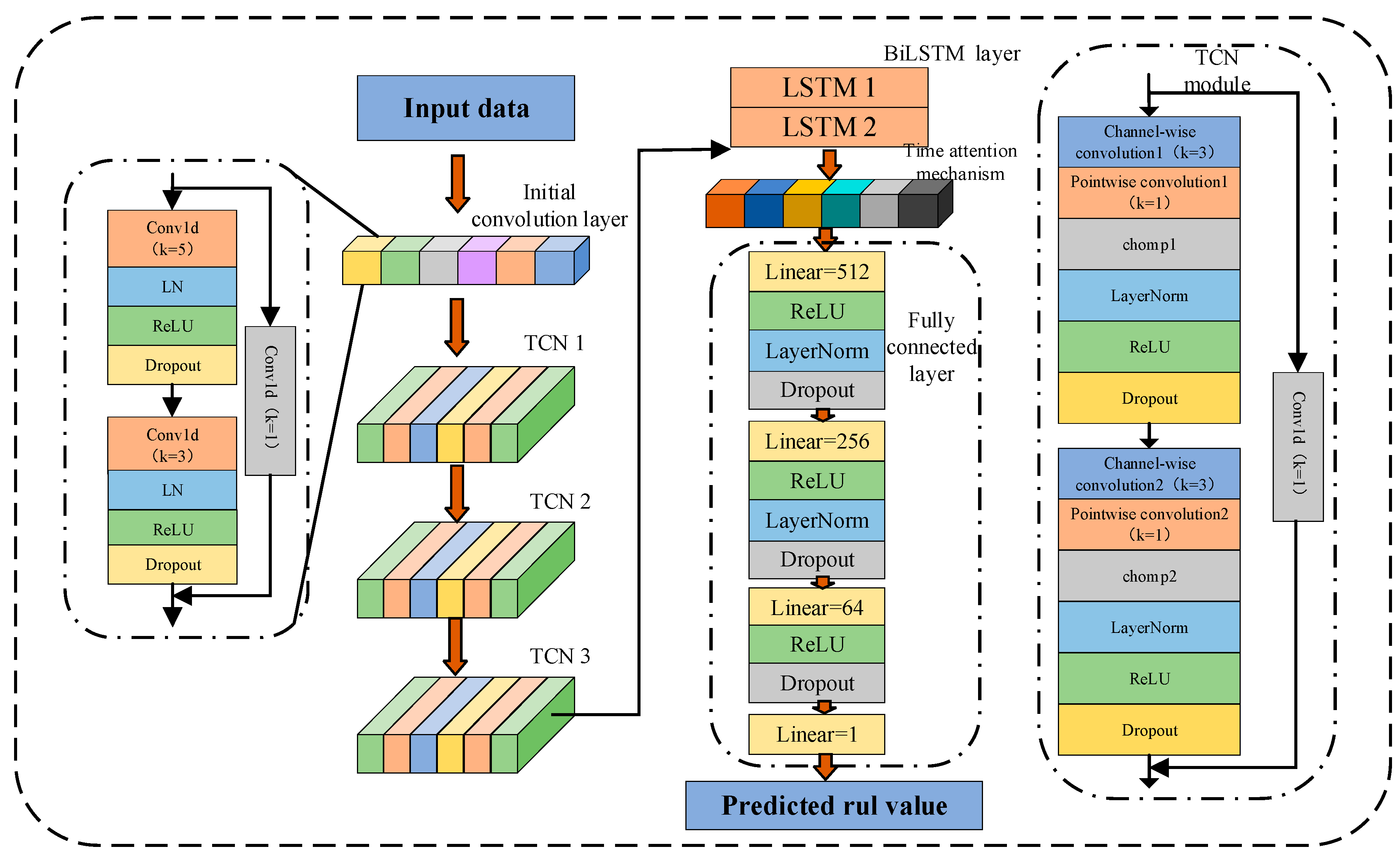
The overall architecture of the TCN-BiLSTM-Attention model proposed in this paper is shown in Figure 1, which consists of five parts: an initial convolutional layer, a TCN layer, a BiLSTM layer, a temporal attention mechanism layer, and a fully connected layer.

The input experimental data is first passed through the initial convolutional layer for low-level feature extraction and channel mapping. Through two layers of one-dimensional convolution operations, combined with processing methods such as LayerNorm, ReLU, and Dropout, smoother and more distinguishable local information can be extracted. Meanwhile, the residual connection structure is introduced to improve the training stability and information retention ability of the network. Then, the TCN layer further extracts local features and medium- and long-term dependencies in the input signal. The combination of causal convolution and dilated convolution can expand the receptive field while maintaining temporal consistency. The main function of the BiLSTM module is to model the bidirectional temporal dependencies in the output sequence of the TCN. Compared with the unidirectional LSTM, the bidirectional structure can simultaneously capture the context information between the current moment and its previous and subsequent states, enabling the model to more comprehensively understand the dynamic change process of the time series. The final fully connected regression module is used to map the context vector output by the attention mechanism to specific lifespan prediction values. This module adopts a multi-layer linear layer structure, combined with ReLU activation, LayerNorm, and Dropout, which enhances the model’s non-linear expression ability and anti-overfitting ability, thus ensuring that the output results still maintain high accuracy and stability under complex industrial conditions.

2.2. Optimization of TCN Networks

The Temporal Convolutional Network (TCN) is a deep learning model constructed based on the Convolutional Neural Network (CNN), which is suitable for the modeling tasks of sequential data such as time series [26]. In this study, the depthwise separable convolution was introduced into the TCN network on the basis of the traditional structure to replace the standard one-dimensional convolution, thereby significantly reducing the number of parameters and computational complexity of the model. The network still retains the design of causal convolution and dilated convolution, enabling the model to effectively expand the receptive field and capture long-term dependency information through a relatively shallow network structure while maintaining temporal consistency. In addition, the TCN also adopts residual connections to further improve the training stability and expressive ability. Compared with the traditional Recurrent Neural Network (RNN), the TCN has obvious advantages in parallel computing ability and long-sequence modeling effect.

2.2.1. Depthwise Separable Convolution

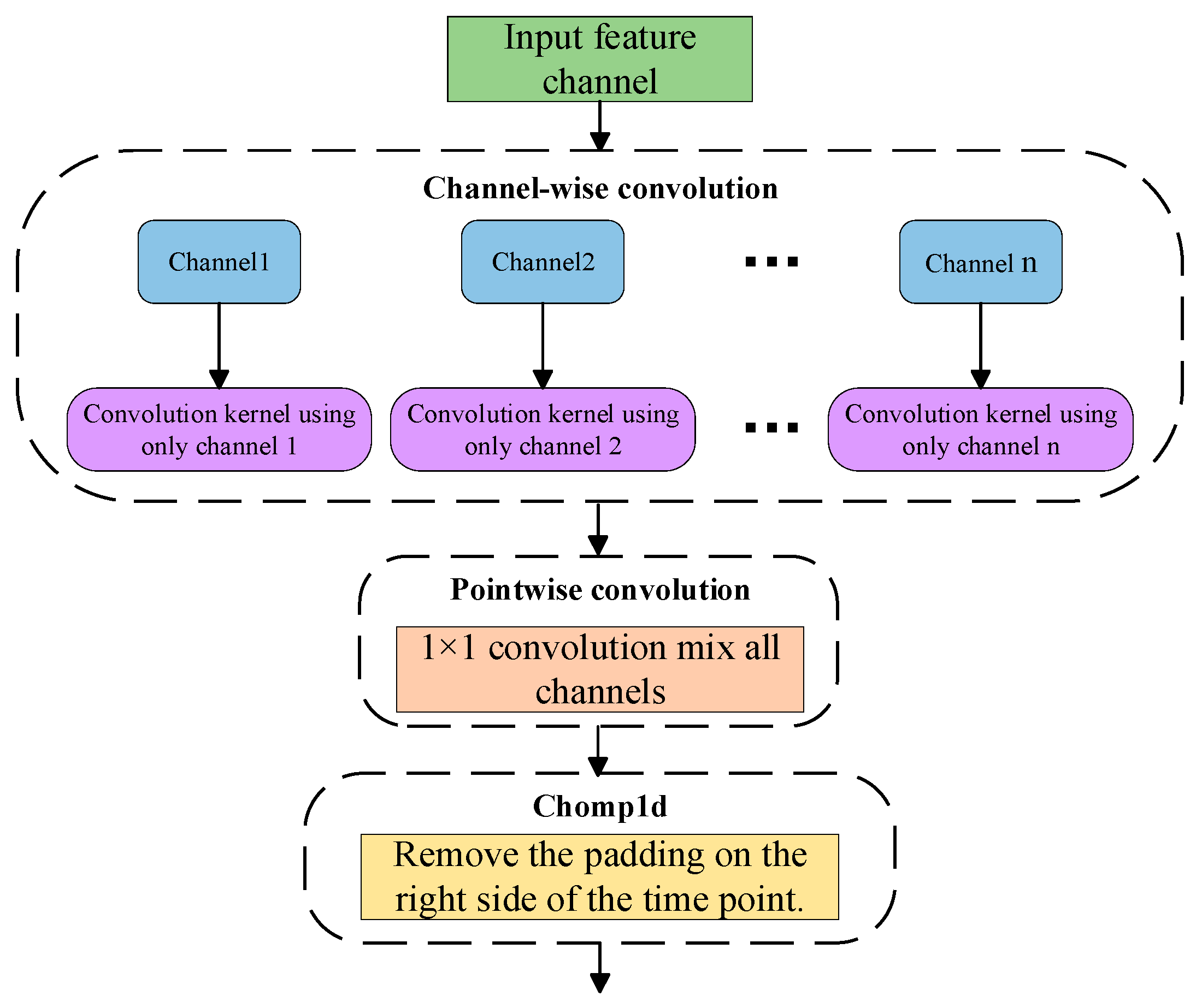
In traditional convolution, standard one-dimensional convolution jointly operates on both the temporal and channel dimensions when modeling the input sequence. Although it has strong expressive power, it also leads to high parameter redundancy and increased computational complexity. Therefore, depthwise separable convolution is introduced, which can separate the feature mapping calculations of the spatial and channel dimensions in the standard convolution operation. This significantly reduces the number of model parameters while maintaining prediction performance [27]. Depthwise separable convolution divides the standard convolution into depthwise convolution and pointwise convolution, and its structure is shown in Figure 2.

Depthwise Convolution performs convolution calculations on each input channel independently without cross—channel information fusion. Each output channel is derived solely from the corresponding input channel, and its mathematical expression is:

For the output channel c, the output is:

$$y_c\left(t\right)=\sum _{k=0}^{K-1}{w}_c\left(k\right)\cdot x_c\left(t-d\cdot k\right)$$

(1)

Among them, $x_c\left(t\right)$ represents the input value of the channel $c$ at time $t$; $w_c\left(k\right)$ is the convolution kernel of this channel; $d$ is the dilation rate; and $K$ represents the size of the convolution kernel.

Pointwise Convolution employs 1 × 1 convolution kernels to mix the outputs of each channel in the channel dimension, integrating information among different channels. Its mathematical expression is as follows:

For the output channel j, its value is:

$$z_j\left(t\right)=\sum _{c=1}^{C_{in}}{\theta }_{j,c}\cdot y_c\left(t\right)$$

(2)

Among them, ${\theta }_{j,c}$ represents the weight parameter between channels; $y_c\left(t\right)$ represents the output of the channel $c$ after channel-by-channel convolution; $z_j\left(t\right)$ represents the value of the final output channel $j$ at time $t$; $C_{in}$ represents the number of input channels.

2.2.2. Causal Convolution

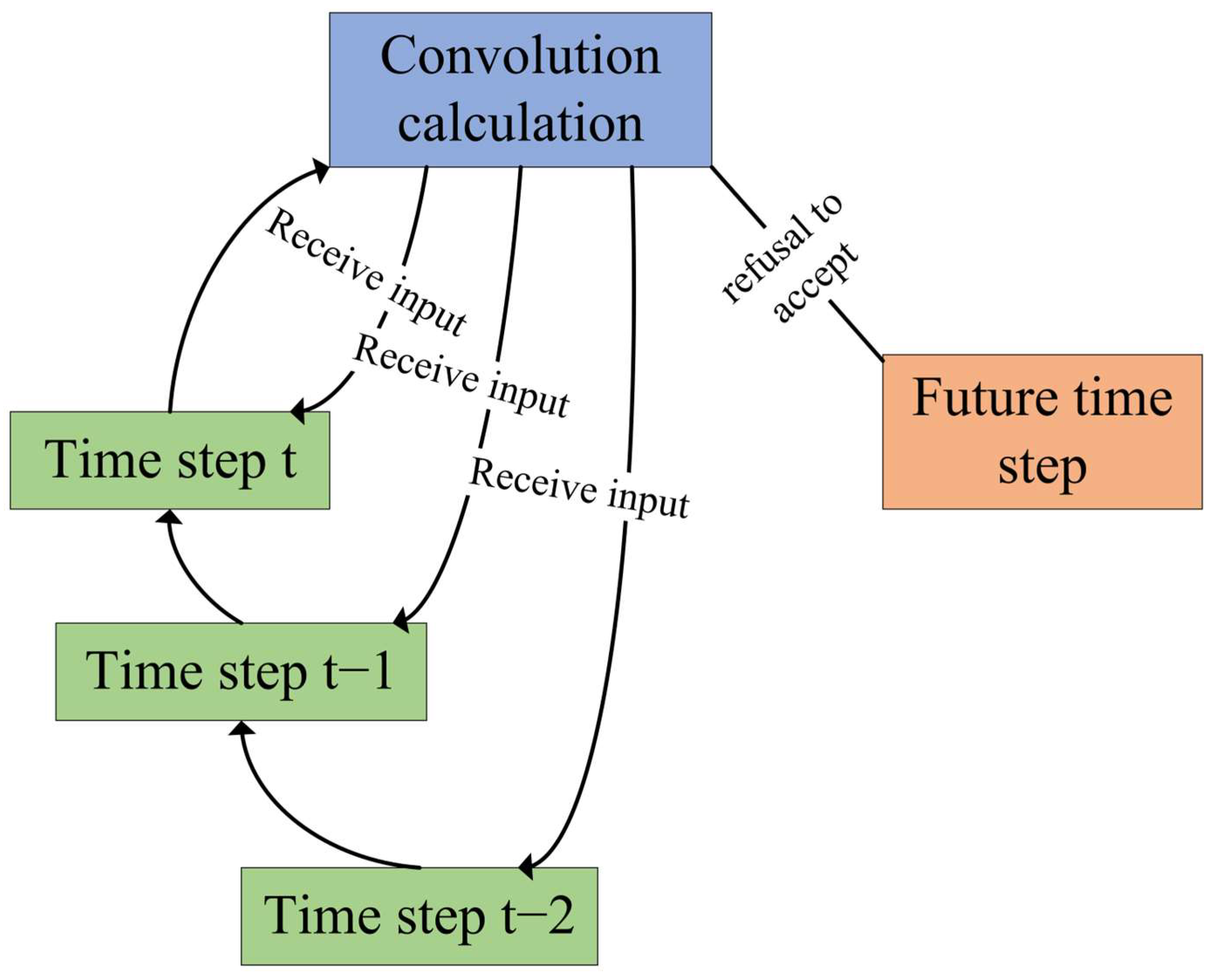
In sequential tasks, to avoid information leakage, TCN employs causal convolution to ensure that the output at each time step only depends on the data at the current time and before, rather than future values. Its structure is shown in Figure 3. The Chomp1d module is used to trim the “future information” introduced by padding in the convolution output. The mathematical expression of causal convolution is:

$$y_t=\sum _{i=0}^{k-1}f\left(i\right)\cdot x_{t-i}$$

(3)

Among them, $t$ represents the current time step; $k$ represents the size of the convolution kernel; $f\left(i\right)$ represents the weight of the convolution kernel at position $i$; $x_{t-i}$ represents the value at time $t-i$ in the input sequence; $y_t$ represents the output at time $t$.

2.2.3. Dilated Convolution

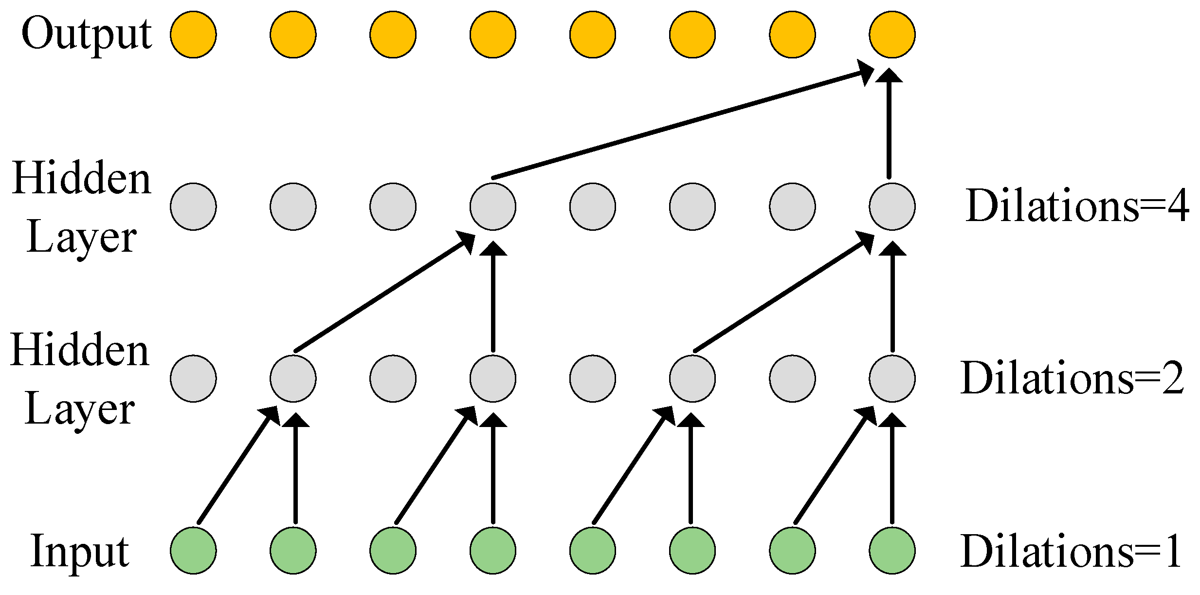
Dilated convolution expands the receptive field significantly without increasing the number of parameters and computational cost by introducing intervals between the sampling points of the convolution kernel, enabling it to capture more abundant contextual information. The structure diagram is shown in Figure 4. The core idea is to insert fixed—interval holes between the sampling points of the convolution kernel, thus expanding the receptive field without increasing the number of parameters. Its mathematical expression is as follows:

$$y\left(t\right)=\sum _{k=0}^{K-1}w\left(k\right)\cdot x\left(t-r\cdot k\right)$$

(4)

Among them, $x$ represents the input sequence; $K$ is the size of the convolution kernel; $r$ is the dilation rate; $w\left(k\right)$ represents the weight of the convolution kernel $k$; $x\left(t-r\cdot k\right)$ denotes the value at a distance of $r\cdot k$ from the current step in the input sequence; $y\left(t\right)$ represents the output at $t$.

2.2.4. Residual Connection

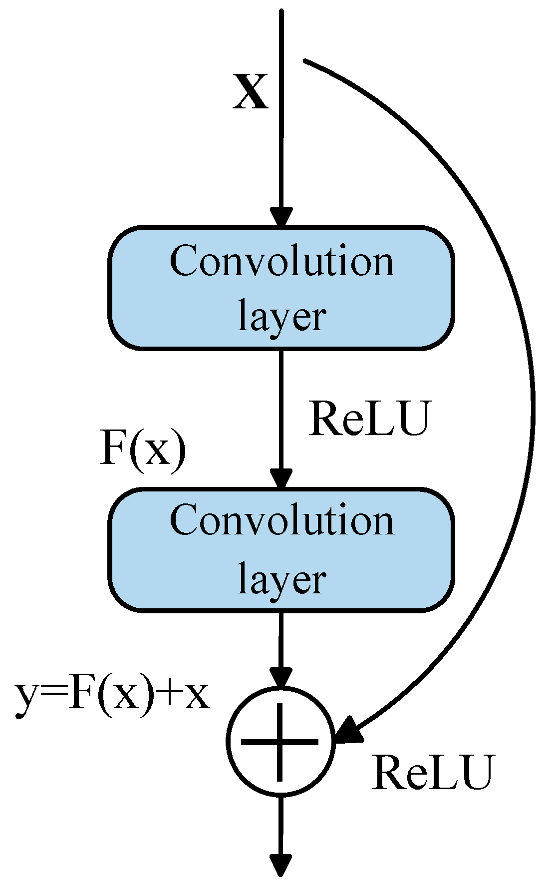
The concept of Residual Connection was proposed to address the issues of vanishing gradients or exploding gradients that occur when the number of layers in a model network increases [28]. A residual connection consists of a main branch and a shortcut path, and its structure is shown in Figure 5. The core idea is to enable the network to learn the residual function rather than directly learning the target mapping function. Its mathematical expression is as follows:

$$y=F\left(x\right)+x$$

(5)

Among them, $F\left(x\right)$ represents the residual mapping learned by the main branch; $x$ represents the original input; $y$ represents the final output.

2.3. BiLSTM Layer

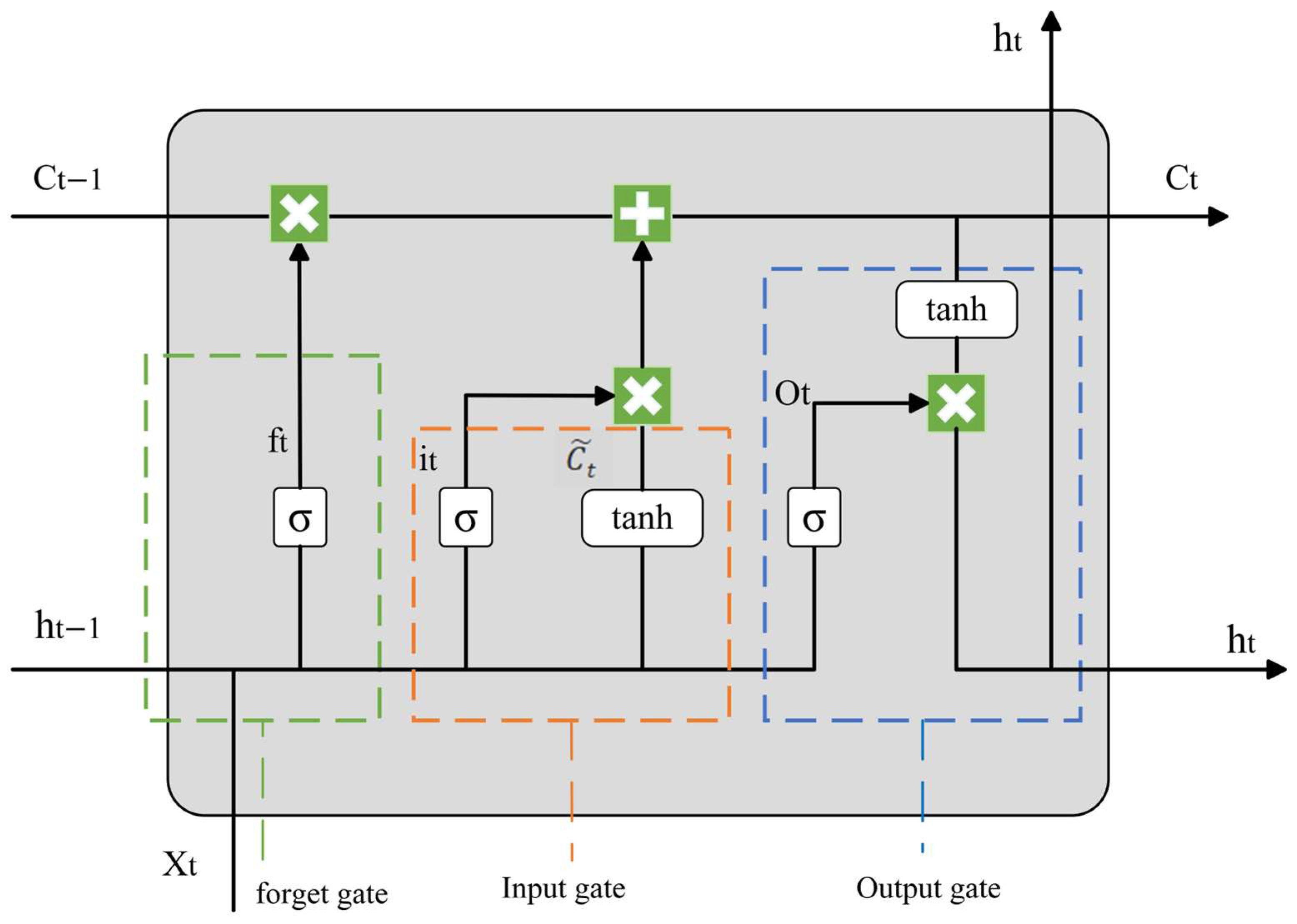
The Long Short-Term Memory (LSTM) network is an improved version of the Recurrent Neural Network (RNN). LSTM can learn long-term dependencies, thus effectively addressing the problems of gradient vanishing and gradient explosion that occur in traditional RNNs when processing long sequences [29]. LSTM mainly determines the retention and forgetting of information through three gating mechanisms, namely: the forget gate, which decides which information will be discarded; the input gate, which determines which new information will be stored in the memory cell; and the output gate, which controls what content will be output. The specific structure is shown in Figure 6, and its mathematical expressions are as follows:

$$\left\{\begin{array}{ll}{f}_t=\sigma \left(W_f\cdot \left[h_{t-1},x_t\right]+b_f\right)& \\ i_t=\sigma \left(W_i\cdot \left[h_{t-1},x_t\right]+b_i\right)& \\ {\tilde{C}}_t=\mathrm{t}\mathrm{a}\mathrm{n}\mathrm{h}\left(W_c\cdot \left[h_{t-1},x_t\right]+b_c\right)& \\ C_t=f_t\odot C_{t-1}+i_t\odot {\tilde{C}}_t& \\ O_t=\sigma \left(W_o\cdot \left[h_{t-1},x_t\right]+b_o\right)& \\ h_t=O_t\odot \mathrm{t}\mathrm{a}\mathrm{n}\mathrm{h}\left(C_t\right)& \end{array}\right.$$

(6)

Among them, $f_t$ represents the output of the forget gate, $\sigma$ represents the Sigmoid activation function, $W_f$ and $b_f$ represent the weights and biases of the forget gate, $h_{t-1}$ is the hidden state of the previous time step, and $x_t$ represents the input of the current time step. $i_t$ represents the output of the input gate, ${\tilde{C}}_t$ represents the candidate cell state, $C_{t-1}$ and $C_t$ are the old and new cell states, and $\odot$ represents element-wise multiplication. $O_t$ represents the result of the output gate, and $h_t$ represents the hidden state of the current time step.

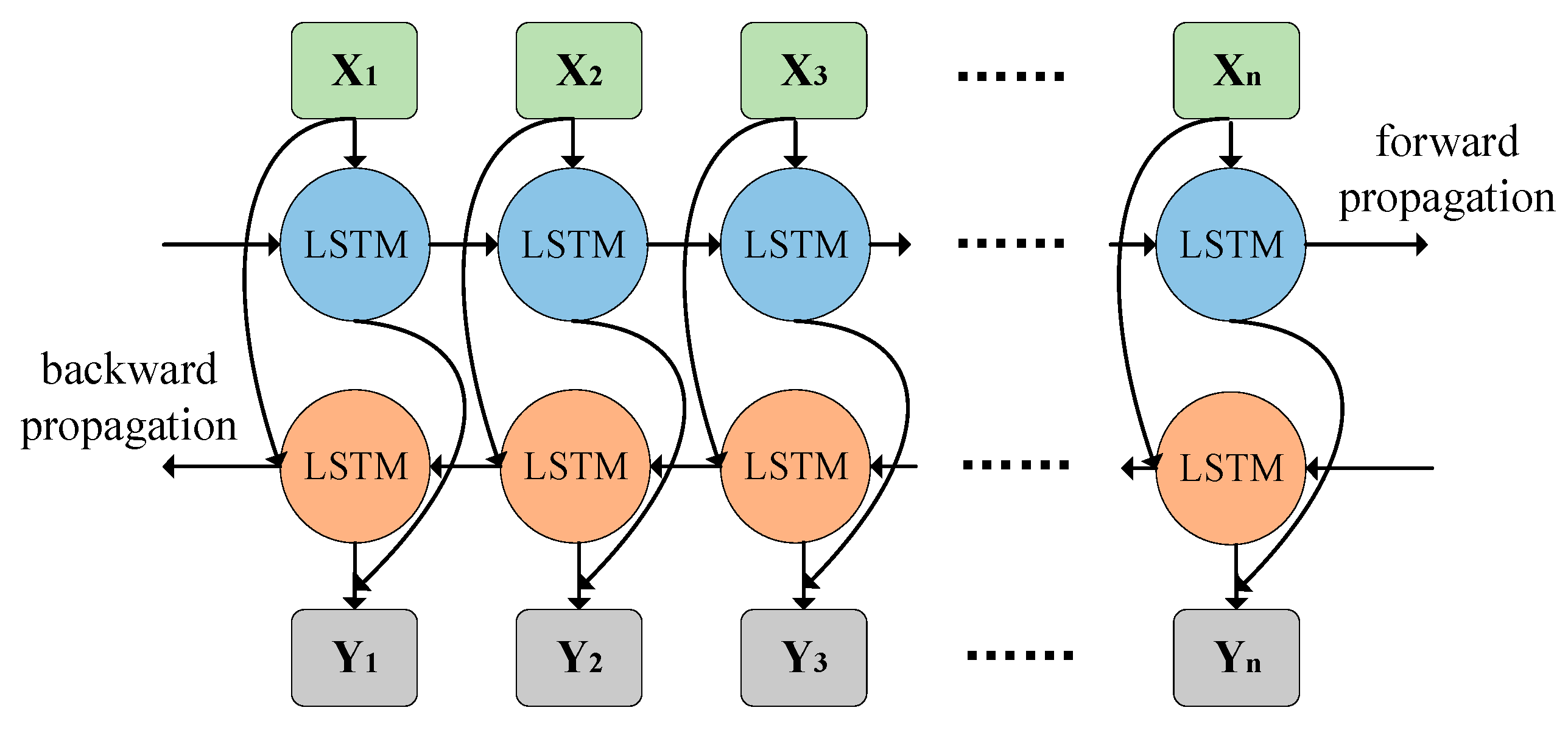
The Bidirectional Long Short-Term Memory network (BiLSTM) introduces a reverse LSTM based on the traditional LSTM. By simultaneously modeling the forward and backward sequence dependencies, it not only enhances the ability to model the global context but also alleviates the long-distance dependency problem, achieving more accurate prediction results. Its structure is shown in Figure 7.

2.4. Temporal Attention Mechanism—Temporal Attention

To enhance the model’s ability to model key time segments, the Temporal Attention mechanism [30] is introduced. This mechanism effectively improves the model’s perception of important time steps without significantly increasing the computational complexity. Its core idea is to dynamically calculate attention weights at each time step of the sequence. All time segments are evaluated through an additive scoring function, and different weights are assigned according to their relative importance. Finally, by performing a weighted sum on the output sequence of the BiLSTM, a context representation rich in global information is extracted. This process enables the model to focus more on the time periods that have a significant impact on the prediction task, thereby improving the overall modeling performance. The computational process of this mechanism is shown in Figure 8.

In the attention mechanism, the attention weights are obtained by scoring the output of the BiLSTM layer at the i-th time step of the sequence, followed by softmax normalization. The specific formulas are as follows:

$$\left\{\begin{array}{l}{z}_t^{\left(1\right)}=\tanh \left(W_1{h}_t+b_1\right)\\ z_t^{\left(2\right)}=\tanh \left(W_2{z}_t^{\left(1\right)}+b_2\right)\\ e_t=W_3{z}_t^{\left(2\right)}+b_3\\ {\alpha }_t={\displaystyle \frac{\exp \left(e_t\right)}{{\displaystyle {\sum }_{k=1}^T\exp \left(e_k\right)}}},{\displaystyle \sum _{t=1}^T{\alpha }_t=1}\end{array}\right.$$

(7)

where T denotes the sequence length; $W_1,b_1$; $W_2,b_2$; $W_3,b_3$ are learnable parameters of the MLP; tanh is the activation function; ${\alpha }_t$ is the scoring scalar at the t-th time step; represents the attention weight at the t-th time step, ranging between 0 and 1, with the sum of all equal to 1.

After calculating the attention weights, a weighted sum of the hidden states at each time step is performed to obtain the context vector. The specific formula is as follows:

$$c={\displaystyle \sum _{t=1}^T{\alpha }_t{h}_t}$$

(8)

where c denotes the context vector, which aggregates the information of the “more important” time steps in the entire sequence for use in the subsequent fully connected layers; $h_t$ represents the output of the BiLSTM at the t-th time step.

2.5. Model Parameters

The parameters of the model are shown in

Table 1. Model parameters.

Parameter Name	Value	Parameter Name	Value
Initial number of convolutional channels	32	Convolution kernel size	[5, 3]
TCN channel structure	[64, 128, 256]	TCN step size	1
Kernel size of TCN	3	Expansion rate	[1, 2, 4]
Number of BiLSTM layers	2	Number of LSTM hidden units	128
Fully connected structure	[512, 256, 64, 1]	Dropout ratio	Initial/TCN: 0.3, FC: 0.2/0.05

. The activation function used in the structure is ReLU, and the normalization method is layer normalization (LayerNorm). After replacing the standard convolution in the TCN network with depthwise separable convolution, the total number of model parameters is reduced from 1,548,418 to 1,293,058. The reduction in the number of parameters improves training efficiency.

3. Experimental Design and Result Discussion

3.1. Introduction to the Experimental Dataset

The experimental data were obtained from the open-source data of the 2010 High-speed CNC Machine Tool Health Prediction Competition organized by the Prognostics and Health Management Society (PHM) in New York, NY, USA [31]. The machining parameters of the experiment are shown in

Table 2. Processing parameters.

Cutting Parameters	Value
Spindle speed (r/min)	10,400
Feed rate (mm/min)	1555
Axial cutting depth/mm	0.2
Radial cutting width/mm	0.125
Sampling frequency/kHz	50
Milling length/mm	108
Single-pass feed amount/mm	0.001
Workpiece material	Inconel 718 rectangular stainless steel

.

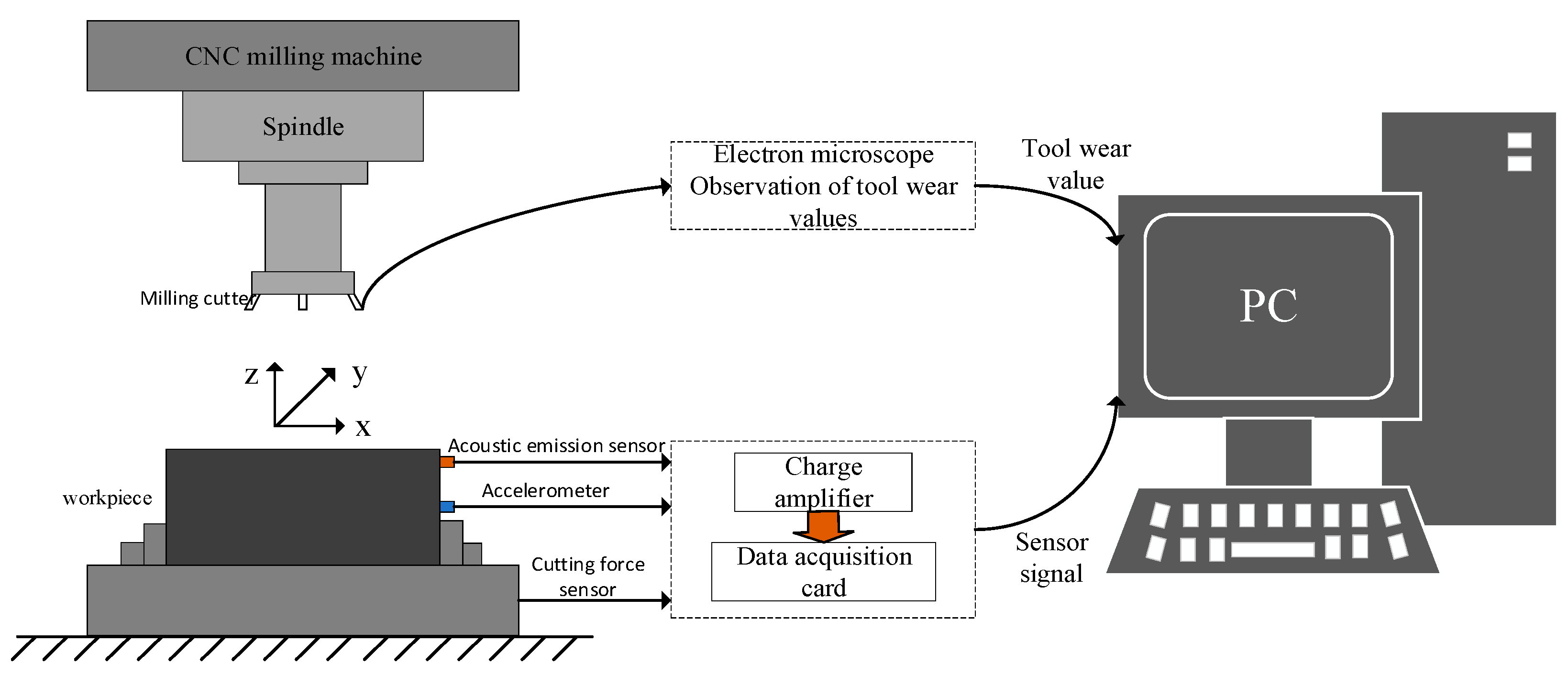
The cutting experiments were conducted on a CNC milling machine. Cutting force, vibration, and acoustic emission sensors were used to collect data during the machining process. The collected data included three-directional cutting force signals, three-directional vibration signals, and acoustic emission signals. The data acquisition process is shown in Figure 9. A total of 6 cutting tools were used in the experiments, and each tool performed 315 passes. Therefore, the PHM 2010 dataset contains 6 corresponding data subsets, namely c1, c2, c3, c4, c5, and c6. The specific parameters of the equipment used in the experiments are listed in

Table 3. Equipment parameters.

Equipment Name	Model and Parameters
Computer Numerical Control (CNC)	Roders Tech RFM760
Cutting force sensor	Kistler 9265B three-axis dynamometer
Vibration sensor	Kistler 8636C three-axis acceleration sensor
Acoustic emission sensor	Kistler acoustic emission sensor
Microscope	LEICA MZ12
Charge amplifier	Kistler 5019A Multi-Channel Charge Amplifier
Data acquisition card	NIDAQPCI1200
Cutting tools	Carbide ball-nose three-flute end mill

.

The raw data after collection is bloated and of poor quality, so it needs to be appropriately preprocessed before being input into the model for training. The preprocessing method adopted in this paper is generally divided into three steps:

• Removal of abnormal data: During model training, since the processes of tool entry and exit are of no help to the model training, the first and last 2.5% of the data of all signals in each pass are removed. The removed signal data is denoised using the wavelet threshold denoising method to improve the reliability of the signal data. The soft threshold method is adopted, and the signal is decomposed into 3 levels using the Daubechies 6 (db6) wavelet basis function. The inter-quartile range (IQR) method is used to remove the outliers in the denoised data, and the IQR threshold is set to 2.
• Data dimensionality reduction: The data after the outlier removal operation is basically clean. However, since the data set is large, directly inputting it into the model for training will significantly increase the training time. Therefore, an equidistant interval sampling method is applied to the data, where 1000 data points are extracted at equal intervals from each column of data. This approach not only simplifies the data but also captures the signal trend. The shape of the processed overall data is [315, 1000, 7].
• Data normalization: To prevent the model from favoring features with larger numerical ranges during training, the min-max normalization is employed to keep all data within the range of 0 to 1. This ensures that the model can treat the data of each channel equally, thereby enhancing the learning efficiency and accuracy of the model.

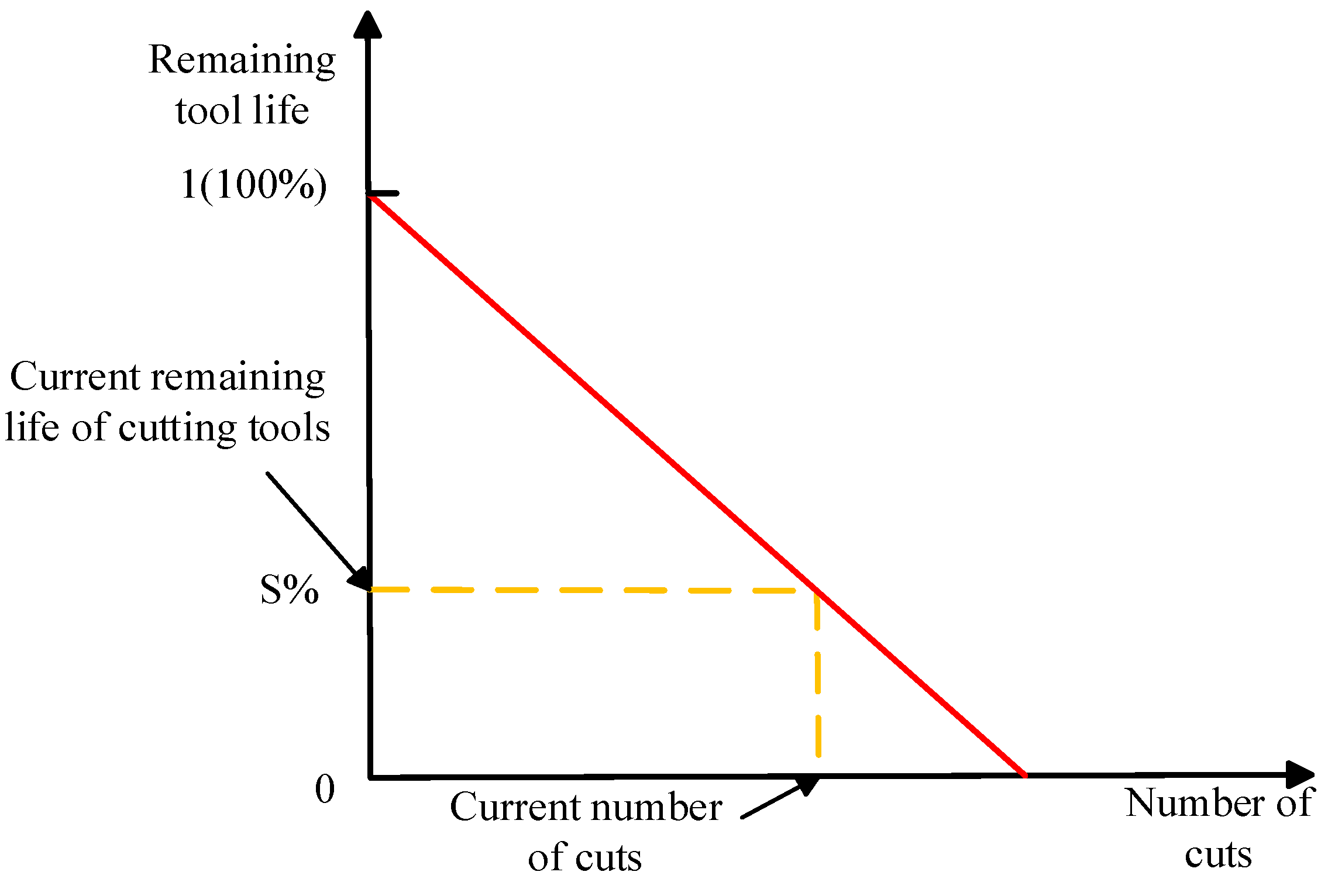
The calculation method of the remaining useful life of the cutting tool is to divide the remaining useful life at the current moment by the total number of machining operations. As shown in Figure 10, the clear relationship between the remaining useful life of the cutting tool and the number of tool passes can be seen from the figure, which more intuitively demonstrates the current health status of the cutting tool.

3.2. Training Methods and Parameter Settings

In this paper, the c1, c4, and c6 datasets are used, and the three-fold cross-validation method is employed for training and validation. Two groups are used for training and the remaining one for testing in each experiment, and a total of three groups of experiments are conducted. During model training, RMSE with L2 regularization is used as the loss function, and the Adamw optimizer is adopted to update the network weights. The specific training parameters are shown in

Table 4. Model training parameters.

Parameter Names	Parameter Values
Loss function	RMSE
Epochs	200
Learning rate	0.0005
Batch	32
Learning rate regulator	ReduceLROnPlateau

.

3.3. Performance Indicators

The performance metrics used for model training and evaluation are the root mean square error (RMSE) [32], mean absolute error (MAE) [33], and coefficient of determination (R²) [34]. When the RMSE and MAE in the results are smaller and the R² is larger, it indicates that the model has good performance and high prediction accuracy.

$$\begin{array}{rr}& RMSE=\sqrt{{\displaystyle \frac{1}{n}}{\displaystyle \sum _{i=1}^n}{\left({\widehat{y}}_i-y_i\right)}^2}\end{array}$$

(9)

$$MAE={\displaystyle \frac{1}{n}}\sum _{i=1}^n\left|{\widehat{y}}_i-y_i\right|$$

(10)

$$\begin{array}{rr}& R^2=1-{\displaystyle \sum _{i=1}^N}{\left({\widehat{y}}_i-y_i\right)}^2/{\displaystyle \sum _{i=1}^N}{\left({\overline{y}}_i-y_i\right)}^2\end{array}$$

(11)

Among them, $y_i$ represents the actual remaining useful life, ${\widehat{y}}_i$ represents the predicted remaining useful life, and ${\overline{y}}_i$ represents the average value of the actual remaining useful life.

3.4. Ablation Experiment

To validate the effectiveness of the model, an ablation experiment was conducted to verify the importance of each module in the model. The proposed model was compared with the model without the temporal attention mechanism (TCN-BiLSTM), the model without the TCN layer (BiLSTM-Attention), and the model without the BiLSTM layer (TCN-Attention), respectively. The initial convolutional layer and the fully-connected layer of the model remained unchanged. The model training method, training parameters, and performance metrics used were kept consistent.

All the above experiments were conducted using the Windows 11 operating system. The model training adopted the deep learning framework PyTorch 2.3.0 with Python 3.8.19. For the hardware, a 13th Gen Intel(R) Core(TM) i7-13620H @ 2.40 GHz processor was used, with 16 GB of memory, a 1 TB solid-state drive (SSD), and an NVIDIA GeForce RTX 4050 graphics processing unit (GPU) as the graphics card.

In Figure 11, Figure 12, Figure 13 and Figure 14, the abscissa represents the number of cutting cycles, the ordinate represents the RUL value, the blue line denotes the predicted RUL value, the red line denotes the true RUL value, and the green squares represent the absolute error between the two. From the prediction performances of each model on the c1, c4, and c6 datasets in Figure 11, Figure 12, Figure 13 and Figure 14, it can be seen that the model proposed in this paper performs best on the three datasets, with the prediction results basically fitting the real-value curve, and only a very small part has relatively large error fluctuations. Compared with the prediction results of the TCN-BiLSTM model (see Figure 11 and Figure 12), the prediction curve of the TCN-BiLSTM model becomes more volatile, and the error also increases. This indicates that after completing the extraction of time-series features, combining the time-series attention mechanism to dynamically weight the features helps to improve the stability and accuracy of the model prediction.

Table 5. Comparison of performance metrics results of various models in ablation experiments.

Model	c1 Dataset			c4 Dataset			c6 Dataset
	RMSE	MAE	R2	RMSE	MAE	R2	RMSE	MAE	R2
Proposed model	0.0282	0.0192	0.9905	0.0184	0.0127	0.9959	0.0431	0.0338	0.9777
TCN-BiLSTM	0.0395	0.0319	0.9813	0.0318	0.0248	0.9879	0.0678	0.0555	0.9448
TCN-Attention	0.0489	0.0307	0.9713	0.0287	0.0211	0.9901	0.0853	0.0663	0.9127
BiLSTM-Attention	0.0520	0.0313	0.9676	0.0261	0.0198	0.9918	0.0979	0.0777	0.8851

presents the specific performance indicators of each model on three datasets. As can be seen from the table, the model proposed in this paper has the smallest RMSE and MAE values and the largest R² value, which also demonstrates the effectiveness of the structure proposed in this paper. In the three-fold cross-validation, the proposed model in this study exhibits the lowest mean and smallest standard deviation across the three metrics of RMSE, MAE, and R² (RMSE = 0.0299 ± 0.0103, MAE = 0.0219 ± 0.0088, R² = 0.9876 ± 0.0071), indicating that the model not only achieves higher accuracy but also possesses better stability and generalization ability across different folds.

The total training times of each model in the ablation experiments are as follows: TCN-BiLSTM-Attention (1263.16 s), TCN-BiLSTM (1190.53 s), TCN-Attention (469.27 s), and BiLSTM-Attention (740.02 s). From the experimental results, it can be observed that the proposed model in this study achieves the best performance among all comparative models, but its training time is also relatively the longest. With the gradual removal of different modules from the model structure, the prediction performance of the model decreases gradually, while the training time is significantly reduced. This indicates that the improvement of model performance is closely related to structural complexity—i.e., although a more complex network structure increases computational overhead, it can more fully capture temporal features, thereby achieving better prediction results.

3.5. Experimental Comparative Analysis

To more fully verify the superior performance of the model proposed in this paper, the TCN, ResNet-BiGRU, and CNN-LSTM models are selected for experimental comparative analysis. The TCN model uses the same parameter settings as those in the model proposed in this paper. In the ResNet-BiGRU model, the residual network uses a convolution kernel of size 3, the number of output channels is 64, and the number of hidden layer units of each GRU layer is 64. In the CNN-LSTM model, the CNN consists of four convolutional layers, the size of the convolution kernel of each layer is 3, the final number of output channels is 64, and the number of hidden layer units of the LSTM is 256. Since all the comparison models are deep learning models, the training parameter settings remain unchanged.

Figure 15, Figure 16 and Figure 17 present the prediction results of the TCN, ResNet-BiGRU, and CNN-LSTM models on the c1, c4, and c6 datasets. As can be seen from the figures, the three models perform well overall on the c1 dataset. However, during the 300th to 315th tool passes, their prediction errors increase significantly. On the c4 dataset, the prediction results of the TCN model start to deviate significantly from the true values after the 150th tool pass. In contrast, the predictions of the ResNet-BiGRU and CNN-LSTM models are closer to the true curve, with the CNN-LSTM model performing relatively better, which may be attributed to its more convolutional layers and stronger feature extraction ability. On the c6 dataset, both the TCN and CNN-LSTM models exhibit varying degrees of prediction deviation, while the prediction curve of the ResNet-BiGRU model fluctuates violently around the true value, indicating poor stability. Overall, the TCN-BiLSTM-Attention model shows the best comprehensive performance on the three datasets, suggesting that the structures such as causal convolution, dilated convolution, and residual connection it employs have stronger modeling ability and robustness in time series prediction tasks.

From the comparison of the performance results in

Table 6. Comparison of performance metrics results of various models in experiments.

Model	c1 Dataset			c4 Dataset			c6 Dataset
	RMSE	MAE	R2	RMSE	MAE	R2	RMSE	MAE	R2
Proposed model	0.0282	0.0192	0.9905	0.0184	0.0127	0.9959	0.0431	0.0338	0.9777
TCN	0.0573	0.0342	0.9607	0.0738	0.0576	0.9347	0.0599	0.0471	0.9569
ResNet-BiGRU	0.0937	0.0467	0.8947	0.0464	0.0357	0.9742	0.0468	0.0381	0.9737
CNN-LSTM	0.0960	0.0329	0.8895	0.0716	0.0538	0.9385	0.0677	0.0508	0.9449

, it can be seen that the TCN-BiLSTM-Attention model proposed in this paper outperforms other comparison models in terms of RMSE, MAE, and R² metrics on three datasets, showing the best prediction performance. On the C1 dataset, the R² of our model reaches 0.9905, significantly higher than that of other models, indicating its stronger fitting ability. On the C4 and C6 datasets, it also achieves R² values of 0.9959 and 0.9777 respectively, maintaining a high level of stability and accuracy.

From the means and standard deviations calculated from the specific data in the table, it can be concluded that the proposed model in this study performs optimally across all three metrics with the smallest standard deviations (RMSE = 0.0299 ± 0.0103, MAE = 0.0219 ± 0.0088, R² = 0.9877 ± 0.0071), indicating that the model possesses excellent stability and robustness under different data partitions. In contrast, the BiGRU model ranks second in all metrics; the TCN model demonstrates moderate performance, while the ResNet and CNN-LSTM models have relatively large standard deviations, indicating significant performance fluctuations under different data partitions. Overall, the proposed model outperforms the other comparative models in both accuracy and stability.

The total training times of each model in the comparative experiments are as follows: TCN-BiLSTM-Attention (1263.16 s), TCN (337.85 s), ResNet-BiGRU (62.32 s), and CNN-LSTM (76.04 s). As indicated by the experimental results, due to its relatively complex structure and larger number of parameters, the proposed model in this study has the longest training time, but it also achieves the optimal prediction accuracy. In contrast, the other three comparative models have relatively simple structures and fewer parameters; although their training times are significantly shortened, their prediction accuracy is also reduced.

4. Conclusions

(1)

This paper proposes a hybrid model framework that integrates an improved TCN network, BiLSTM network, and temporal attention mechanism to predict the remaining useful life of cutting tools. The accuracy and reliability of the model are verified using the PHM 2010 dataset. In three groups of experiments, the performance indicators of the proposed model are as follows: RMSE: 0.0282, 0.0184, and 0.0431; MAE: 0.0192, 0.0127, and 0.0338; R²: 0.9905, 0.9959, and 0.9777. The values of these three performance indicators demonstrate the prediction accuracy and reliability of the model.

(2)

The model proposed in this paper fully leverages the advantage of the improved TCN in extracting local temporal patterns and the modeling ability of BiLSTM in capturing long-distance dependencies. Meanwhile, the attention mechanism further enhances the model’s ability to focus on key time segments, achieving adaptive selection and weighted modeling of high-dimensional temporal information. Through the ablation experiments and model comparison experiments conducted on the PHM 2010 dataset, the reliability of the model architecture proposed in this paper and the accuracy of its prediction can be observed.

In future research, the model will be applied to practical scenarios such as real-time condition monitoring, and its prediction performance will be further verified through long-term on-site tests. Although the prediction accuracy of the model proposed in this paper is relatively good, the training and validation are all carried out under a single process. In the future, cutting parameters, machining paths, etc., can be incorporated into the input data under multiple processes for training and validation in combination with transfer learning. The influence of different workpiece materials on the model’s prediction performance can also be studied.