Article

Hybrid ML-Based Cutting Temperature Prediction in Hard Milling Under Sustainable Lubrication

by
Balasuadhakar Arumugam
1,
Thirumalai Kumaran Sundaresan
2,* and
Saood Ali
3,*
1
Department of Mechanical Engineering, Sona College of Technology, Salem 636005, Tamil Nadu, India
2
Department of Mechanical Engineering, PSG Institute of Technology and Applied Research, Coimbatore 641062, Tamil Nadu, India
3
School of Mechanical Engineering, Yeungnam University, 280 Daehak-Ro, Gyeongsan 38541, Gyeongbuk, Republic of Korea
*
Authors to whom correspondence should be addressed.
Lubricants 2025, 13(11), 498; https://doi.org/10.3390/lubricants13110498
Submission received: 26 September 2025 / Revised: 28 October 2025 / Accepted: 12 November 2025 / Published: 14 November 2025

Abstract

The field of hard milling has recently witnessed growing interest in environmentally sustainable machining practices. Among these, Minimum Quantity Lubrication (MQL) has emerged as an effective strategy, offering not only reduced environmental impact but also economic benefits and enhanced cooling performance compared to conventional flood cooling methods. In hard milling operations, cutting temperature is a critical factor that significantly influences the quality of the finished component. Proper control of this parameter is essential for producing high-precision workpieces, yet measuring cutting temperature is often complex, time-consuming, and costly. These challenges can be effectively addressed by predicting cutting temperature using advanced Machine Learning (ML) models, which offer a faster and more efficient alternative to direct measurement. In this context, the present study investigates and compares the performance of Conventional Minimum Quantity Lubrication (CMQL) and Graphene-Enhanced MQL (GEMQL), with sesame oil serving as the base fluid, in terms of their effect on cutting temperature. The experiments are structured using a Taguchi L36 orthogonal array, with key variables including cutting speed, feed rate, MQL jet pressure, and the type of cooling applied. Additionally, the study explores the predictive capabilities of various advanced ML models, including Decision Tree, XGBoost Regressor, K-Nearest Neighbor, Random Forest Regressor, and CatBoost Regressor, along with a Hybrid Stacking Machine Learning Model (HSMLM) for estimating cutting temperature. The results demonstrate that the GEMQL setup reduced cutting temperature by 36.8% compared to the CMQL environment. Among all the ML models tested, HSMLM exhibited superior predictive performance, achieving the best evaluation metrics with a mean absolute error of 3.15, root mean squared error (RMSE) of 5.3, mean absolute percentage error of 3.9, coefficient of determination (R2) of 0.91, and an overall accuracy of 96%.

1. Introduction

AISI H11 hot work tool steel is widely used for machining tools, dies, hot shear blades, and aerospace components because of its high hardness, toughness, wear resistance, and reliable performance under high stress and elevated temperatures [1]. Milling is a versatile machining process that produces flat, helical, and curved surfaces. The main challenges in hard milling are significantly reduced tool life and compromised surface quality [2]. In hard milling, lubrication is vital for limiting friction and dissipating heat at the contact zone between the tool and the workpiece, which helps maintain tool performance and improves the machined surface [3]. Minimum Quantity Lubrication (MQL) technique enhances sustainability in the milling process by using minimal lubricant, thereby cutting down fluid waste and disposal issues. It further contributes to eco-friendly machining through reduced resource usage and lower environmental footprint [4]. Due to their renewable origin, biodegradability, and eco-friendly characteristics, vegetable oils serve as effective substitutes for mineral cutting fluids. Their application through MQL further promotes green and sustainable machining practices [5].
Studies reveal that nanoparticles enhance lubricant performance by reducing friction and wear. This is achieved through mechanisms like rolling, self-repair, polishing, and tribo-film formation [6]. Haq et al. studied copper-based nanofluid MQL (NMQL) in milling Inconel 718 and found notable improvements, with a 14.7% drop in cutting temperature (Tc), 20.1% reduction in surface roughness (Ra), and 13.3% decrease in power consumption [7]. Pal et al. studied the impact of sunflower oil-based MQL with Al2O3 nanoparticles on the machinability of AISI 321 steel. Their findings indicated substantial reductions in key parameters compared to the conventional flood cooling method, including a 44% decrease in cutting force (Fc), a 67% reduction in torque (T), a 56% reduction in Ra, and a 26% decrease in Tc [8]. Dong et al. investigated the application of MoS2 particles in an emulsion-based MQL system during the machining of SKD11 tool steel and reported a 55% reduction in surface Ra compared to dry machining [9]. Hamdi et al. studied the influence of hexagonal boron nitride (hBN) and multi-walled carbon nanotube (MWCNT) nanofluids in an MQL system with vegetable base oil for machining AISI H11. Compared to dry and pure MQL, MWCNTs lowered Tc and Ra, while hBN reduced energy consumption (Uc) [10].
Sesame oil, derived from sesame seeds, is rich in antioxidants and fatty acids, offering good lubrication and eco-friendly properties. Its biodegradability, availability, and low cost make it a sustainable option for multiple uses [11]. Padmini et al. studied MQL machining of AISI 1040 using sesame and coconut oils with MoS2 additives, finding that sesame oil with nano MoS2 gave the best results, with major reductions in tool wear (VB), Ra and Fc compared to dry cutting [12]. Furthermore, Ni et al. investigated the use of Fe3O4, Al2O3, and carbon nanoparticles dispersed in sesame oil for broaching AISI 1045 steel. Their results indicated that the carbon-based nanofluid exhibited higher viscosity, minimized friction, reduced Fc, lowered vibration, and improved surface finish compared to the others [13]. Graphene nanoplatelets (Gnps), with their two-dimensional layered structure, offer excellent wear resistance and friction-reducing behavior, making them effective micro- and nano-scale lubricants as well as additives in liquid lubricants [14]. Their unique atomic arrangement of carbon atoms in a honeycomb lattice also provides outstanding thermal conductivity. The strong carbon-carbon bonds allow heat to transfer rapidly through lattice vibrations (phonons) with minimal resistance, enhancing lubrication performance in both thermal and mechanical applications [15].
Touggui et al. explored the effectiveness of six distinct cooling conditions, including Gnps-enriched MQL, MoS2-enriched MQL, MWCNT-enriched MQL, Gnps/MoS2 hybrid MQL, MWCNT/MoS2 hybrid MQL, along with dry cutting in the turning of AISI 304 stainless steel. The MQL system employed vegetable oil as its base fluid. The study revealed that Gnps-enriched MQL effectively reduced Ra, Fc, Tc, and VB, achieving greater improvements than other cooling environments, including hybrid nanofluids [16]. Paiva et al. studied the machining performance of SAE 52,100 steel using Gnps-enhanced synthetic and semi-synthetic fluids, in comparison with MQL and flood cooling. Their results revealed that the addition of Gnps led to a 29% reduction in Ra with synthetic oil and a 14% reduction in cutting energy [17]. Similarly, Pal examined the MQL drilling of AISI 321 stainless steel with vegetable-oil-based nanofluid containing Gnps and reported reductions in Fc (27.4%), T (64.9%), Ra (33.8%), and coefficient of friction (51.7%) compared to pure MQL, along with improved tool life [18]. Jiang et al. investigated the micro-bearing effect of Gnps when mixed with SiC in a hybrid nanofluid. Their findings demonstrated that this synergistic combination significantly enhanced the lubrication performance of the coolant [19]. Extending these findings, Li et al. investigated the milling of TC4 alloy using Gnps MQL in combination with a bionic micro-texture tool, which reduced Fc (40%), Tc (43.8%), and Ra (56.9%), while extending tool life by 112% compared to dry cutting [20].
Sustainable manufacturing is rapidly advancing through the adoption of machine learning (ML) and artificial intelligence, where these technologies are being applied to optimize processes, boost productivity, and reduce environmental impact [21]. Mia et al. proposed a predictive ML model based on the Artificial Neural Network (ANN) algorithm for estimating Tc during the turning of AISI 1060 steel under both dry and high cooling conditions. In this model, cutting speed (vc) and feed rate (f) were considered as the primary input variables, and through comparative analysis, the ANN demonstrated superior accuracy over the Response Surface Model, as evidenced by its lower Mean Absolute Error (MAE) values [22]. Building upon this line of research, Gupta et al. conducted a comparative study employing both Response Surface Model and the Adaptive Neuro-Fuzzy Inference System to predict machining responses, including Fc, Tc, and Ra, under NMQL conditions. Their findings indicated that the Adaptive Neuro-Fuzzy Inference System provided enhanced predictive performance compared to the Response Surface Model, thereby highlighting the effectiveness of hybrid soft computing approaches in machining optimization [23].
Furthermore, Zhang et al. advanced this field by developing a Gaussian Process Regression model aimed at forecasting Fc, Ra, and tool life during turning operations. The model utilized vc, f, and depth of cut as its input parameters, and it exhibited remarkable stability and accuracy, establishing itself as a reliable tool for predictive modeling in machining processes [24]. Jurkovic conducted a comparative study of Support Vector Regression (SVR), polynomial regression, and ANN for predicting Ra, Fc, and tool life in high-speed turning, and their result revealed that polynomial regression provided better prediction of Ra and Fc, while ANN resulted in the best prediction of tool life [25]. Another comparative study was conducted by Mahfouz et al. to predict Ra in the end milling of aluminum. The study evaluated the performance of SVR, K-Nearest Neighbor (KNN), and Decision Tree (DT) models, and the results showed that SVR attained the highest accuracy of 81.3% among the models [26]. Additionally, Sizemore developed an ANN model to predict surface roughness during the turning of germanium and compared its performance with DT, RF, AdaBoost, and SVR, demonstrating the competitive capability of ANN-based approaches in machining applications [27].
A pure ML algorithm relies on a single method or technique to address a problem from beginning to end. In contrast, a hybrid algorithm combines two or more approaches, often from different domains, to tackle a task or enhance the efficiency of a single method. Such integration allows hybrid techniques to exploit the advantages of each individual algorithm while compensating for their weaknesses [28]. Akbari et al. developed a physics-informed substructure approach combined with a Bayesian learning algorithm to predict milling machine tool stability in production settings, demonstrating improved accuracy even with limited or suboptimal training data [29]. In a related effort, Rahman et al. devised a physics-guided ML method for predicting the corrosion resistance of alloys, highlighting the growing integration of domain knowledge with data-driven models to enhance prediction reliability [30]. Furthermore, Kim et al. applied a Bayesian learning method integrated with a Deep Multiscale Convolutional Neural Network, achieving significant improvements in forecasting VB during end milling operations [31].
Huange al. introduced two hybrid machine learning models, Particle Swarm Optimization integrated with SVR and Particle Swarm Optimization integrated with Least Squares SVR, to predict VB in milling. These models were compared with conventional SVR. The analysis showed that the hybrid model achieved the best predictive performance, with a mean absolute error of 5.1, a mean absolute percentage error of 0.018, and a root mean square error of 0.018 [32]. Furthermore, Karmi et al. developed three hybrid models, namely optimizer-based deep neural networks, genetic algorithm-based deep neural networks, and deep neural network with extended Kalman filters to predict Fc, Ra, and power consumption during the machining of EN GJL 250 grey cast iron. These hybrid methods were compared with traditional ML models such as SVM, DT, and Levenberg–Marquardt, and the findings showed that the deep neural network with extended Kalman filters achieved the highest predictive performance [33].
A comprehensive review of the existing literature has revealed research gaps in the area of Tc analysis under MQL conditions. Only a limited number of studies have examined this aspect. Additionally, investigations on sesame oil as a cutting fluid are scarce, and work involving Gnps-enriched sesame oil in MQL environments is even more limited. Furthermore, the application of advanced ML models for predicting Tc remains largely unexplored, while the utilization of hybrid ML algorithms in this context is highly limited. Consequently, the present investigation focuses on assessing the performance of Graphene-Enhanced MQL (GEMQL) relative to Conventional Minimum Quantity Lubrication (CMQL), employing sesame oil as the base fluid during the hard milling process. The cutting temperature is selected as the principal response parameter, with the study addressing the influence of f, Vc, lubrication environment, and MQL jet pressure (Pj). In addition, this work seeks to develop a predictive framework for Tc using a Hybrid Stacking Machine Learning Model (HSMLM). The predictive capability of the proposed HSMLM will be benchmarked against advanced ML models.

2. Materials and Methods

2.1. Data Acquisition

In this investigation, AISI H11 hot die steel was selected as the workpiece material. Its chemical composition consisted of C (0.40%), Si (0.98%), Mn (0.25%), P (0.021%), S (0.01%), Cr (4.88%), Mo (1.21%), V (0.42%), with Fe as the remaining balance. The milling trials were performed on an LMW CNC vertical machining center (Model: LV 45), India, as illustrated in Figure 1. A TiAlN-coated carbide end mill cutter was utilized, having four flutes, a diameter of 6 mm, a helix angle of 30°, a flute length of 20 mm, and an overall length of 64 mm [34]. The cutting process was carried out under two lubrication conditions, namely CMQL and GEMQL. A minimum quantity lubrication setup with a reservoir capacity of 3 L supplied the cutting fluid at a constant flow rate of 60 mL/h. Sesame oil was used as the base fluid for the GEMQL condition.
The graphene nanoplatelets (Gnps), procured from a commercial supplier, were incorporated as the nano-additive. Their specifications included a thickness of 5–10 nm, length of 5–10 µm, density of 0.279 g/cm3, surface area ranging from 200–240 m2/g, 4–10 layers, and a thermal conductivity of about 2000 W/m-K. Based on findings from earlier work, the nanofluid was prepared at a concentration of 0.8 wt.% Gnps [35]. The preparation followed a two-step approach: initially, the mixture underwent ultrasonic agitation for 30 min using a Lark ultrasonic bath; subsequently, it was homogenized with an iStir HP 550 magnetic stirrer at 600 rpm for 45 min [36].
Experimental trials were designed using the L36 orthogonal array. The parameters studied included Vc of 40, 50, and 60 m/min, f of 0.01, 0.02, and 0.03 mm/rev, and Pj of 2, 4, and 6 bar, which were selected considering tool manufacturer recommendations and evidence from the literature [37,38]. Tc was recorded by means of a K-type thermocouple linked to an NI DAQ 9212 data acquisition unit, operating at a sampling frequency of 96 samples per second per channel. To improve accuracy, the thermocouple tip was positioned at a uniform distance of 0.5 mm beneath the machined surface, with thermal paste (conductivity >1.93 W/m-K) applied in the gap to ensure efficient heat transfer [39]. Additionally, Tc data were validated using an FLIR E60 infrared thermal imaging camera, India, providing cross-verification for the thermocouple measurements [40].

2.2. Data Preprocessing and ML Model Generation

The dataset used in this study consists of 36 rows and 5 columns, and it is well-structured. It includes one dependent variable, Tc, and four independent variables: cooling condition, Vc, f, and Pj. Data preprocessing and ML models development were performed in Python (Python V3.12.12) using Google Colab. The dataset, stored in CSV format, was imported into the notebook, and its structure was verified by checking its shape, feature details, data types, and null values. The numerical variables Vc, f, and Pj, and Tc were isolated for further analysis. Their distributions were examined using matplotlib distribution plots, while violin plots were employed to detect the presence of outliers.
A correlation heat map was generated to evaluate the association between the dependent variable Tc and the independent variables Vc, f, and Pj. Furthermore, to address the issue of overfitting caused by the limited dataset and to enhance the accuracy of the ML models, Gaussian data augmentation was applied. A noise factor equal to 0.01 was used, the augmentation method employed the fixed random seed of 42 to ensure reproducibility, and the augmentation process was repeated ten times [41]. Subsequently, the independent and dependent variables were separated as x and y. To ensure uniformity, the dataset underwent normalization through the StandardScaler method. Finally, the dataset was divided into training and testing sets, allocating 80% for model training and 20% for evaluation [42].
The DT is a widely used ML method for both regression and classification tasks. It operates as a predictive model by recursively splitting the dataset into subsets according to the most significant features, ultimately forming a tree-like structure. The criterion commonly used for splitting nodes in decision trees is the Gini impurity. It is calculated using the following formula, where kq represents the proportion of samples in the node belonging to class q [43].
I G k = 1 q = 1 Q k q 2
XGBoost is a powerful ML algorithm that combines DT with gradient boosting, providing efficient and precise results for both regression and classification applications [44].
y ^ i t = k = 1 t f k x i = y ^ i t 1 + f t x i
where y ^ i t represents the final constructed tree model; y ^ i t 1 is the tree model generated previously; f t x i denotes the recently produced tree model, and t is the overall count of base tree models. In XGBoost, tree depth and the number of trees are key parameters, and optimization involves finding a classifier that minimizes the chosen loss function, as shown in Equation (3).
o b j t = i = 1 t L y i , y ^ i t + i = 1 t Ω f i
where y i designates the actual value, y ^ i t denotes the predicted value, the loss function is represented by L y i , y ^ i t , and the regularization term is denoted as Ω f i .
The KNN method operates on the principle that data points with comparable characteristics are typically located close together within the feature space. To make predictions, KNN examines the ‘k’ closest instances from the training set and assigns the outcome based on the most common class among those neighbors. Its performance heavily depends on the distance measure used and the selection of an appropriate k value. In addition, the method often demands proper preprocessing, such as feature scaling or normalization, to ensure reliable results [45].
P r e d i c t e d   v a l u e   y ^ = 1 k i = 1 k y i
The Random Forest Regressor (RFR) is an ensemble-based approach capable of handling both regression and classification tasks. It constructs multiple decision trees by repeatedly splitting the dataset into more uniform nodes according to predictor variables. The collective prediction is then derived by averaging the outputs of all trees, thereby enhancing model accuracy [46].
D = x i , y i i = 1 N
D n = x i , y i i n
s p l i t x , , θ = arg   min , θ N l N n V a r D l + N r N n V a r D r
V a r D = 1 D x i , y i D y i y ¯ 2
y ^ m x = 1 D l e a f x i , y i D l e a f y i
y ^ x = 1 m m = 1 M y ^ m x
j = 1 M m = 1 M n o d e   s p l i t   o n   j   V a r D n N l N n V a r D l N r N n V a r D r
y ^ O O B , i = 1 D O O B , i T m i y i y ^ O O B , i 2
where D n is the dataset contained in a node, N n is the count of instances within the node, N l denotes the count of instances in the left side child node, N r is the count of instances in the right side child node, and D l represents the dataset in the left child node, while D r denotes the dataset in the right child node, D l e a f is the set of training instances in the leaf node, j represents the feature importance, and O O B is out-of-bag data.
CatBoost is a gradient boosting algorithm that uses binary decision trees and stands out with ordered boosting, efficient modifications, and strong handling of target leakage, making it well-suited for small datasets. This technique, referred to as Greedy Target-based Statistics, operates by iteratively selecting the most optimal target-based statistics to enhance model accuracy [47]. CatBoost can be described as follows:
j = 1 p x j , k = x i , k y i j = 1 n x j , k = x i , k
Consider a dataset consisting of observations D = X i , Y i   i = 1 , , n , given a permutation σ = σ 1 , σ n , x σ p , k is substituted using the following relation, where p is a prior estimate and a denotes the weight assigned to this prior estimate.
j = 1 p 1 x σ j , k = x σ p , k y σ j + a p j = 1 p 1 x σ j , k = x σ p , k + a
Hyperparameter tuning involves optimizing predefined parameters of a machine learning algorithm that are not learned from data, aiming to improve model performance and generalization. A common method is grid search with cross-validation, which systematically tests combinations of hyperparameters to identify the best-performing setup [48].
Θ = θ 1 , θ 2 , , θ p | θ i ϵ Θ i
D = K = 1 K D k
D T r a i n , k = D D k
M θ k = T r a i n M , D T r a i n , k , θ
P θ k = E x , y D v a l , k L M θ k , x , y
P ¯ θ = 1 k k = 1 K P θ k
σ θ 2 = 1 k 1 k = 1 K P θ k P ¯ θ 2
θ * = arg max θϵ Θ P ¯ θ
θ * = arg max θϵ Θ P ¯ θ λ σ θ
where D represents the dataset and Θ denotes the hyperparameter space, and the dataset is divided into k folds for cross-validation, with D k indicating the k th fold. For each fold k , the training set is designated as D T r a i n , k and the validation set as D v a l , k . The model parameterized by hyperparameters θ for the k th fold is expressed as M θ k , and the performance is assessed using the loss function L . The optimal hyperparameters, θ * , are those that maximize the average performance across all folds. Additionally, a trade-off parameter λ is used to balance mean performance and variance, ensuring robust model evaluation and selection.
Data augmentation (DA) is a strategy used to expand a limited dataset by artificially generating new samples. Among various DA approaches, Gaussian Data Augmentation (GDA) is considered one of the most efficient methods. It enhances the dataset by adding Gaussian noise to existing data points, thereby reducing data scarcity issues and improving the model’s ability to generalize. Applying GDA reduces overfitting, enhances robustness, and boosts prediction accuracy. Gaussian noise is a random variation that adheres to a normal distribution, typically defined by a mean ( α ) of 0 and a standard deviation ( β ) of 1. Here, x represents a random variable drawn from this distribution [49]. The probability density function describing Gaussian noise can be expressed mathematically as follows:
f x = 1 2 π β e x p x α 2 2 β 2 = 1 2 π e x p x 2 2
The proposed Hybrid Stacking Model integrates the strengths of multiple machine learning algorithms to enhance predictive accuracy and robustness, as illustrated in Figure 2. In this framework, both categorical and continuous features are preprocessed using a column transformer, where polynomial interaction terms and standardization are applied to continuous inputs for improved representation. At the base level, diverse learners—including KNN, DT, RFR, XGBoost, and CatBoost—capture varying structural patterns and nonlinear relationships within the data. Their prediction outputs are subsequently combined through a meta-learner, which balances bias–variance trade-offs and mitigates overfitting effects through regularization mechanisms [50].
Additionally, a Transformed Target Regressor with Yeo–Johnson transformation is applied to stabilize variance and normalize the target distribution, ensuring smoother and more consistent model learning. Within this hybrid stacking architecture, layer-wise interaction occurs as the transformed feature vectors propagate through heterogeneous base learners, each capturing complementary predictive signals. The resulting prediction outputs are concatenated with the processed features to construct a richer meta-feature space for second-level learning, wherein the ElasticNet meta-learner assigns optimal weights by amplifying informative predictions while attenuating noisy contributions. During training, errors are iteratively minimized as the meta-learner refines residual patterns that are not captured at the base layer. This hierarchical learning mechanism collectively improves robustness, enhances generalization, and delivers significantly improved predictive performance.
The continuous features are expanded with polynomial interaction terms and then standardized as expressed by:
x ¯ = x = x b , S p o l y x c
The meta-learner combines the base model predictions with the original preprocessed features using the ElasticNet regularization framework:
min β , b 1 2 n z H β + b 2 2 + α λ | β | 1 + 1 λ 1 2 | β | 2 2
The final prediction is obtained by aggregating base learner outputs, applying the meta-learner, and then inverting the target transformation:
y ^ * = T 1 g f 1 ϕ x * , ,   f M ϕ x * , ϕ x *
The binary features are denoted as x b , while the continuous features are represented by x c , including Speed, Feed, and MQL Pressure. The function p o l y . refers to polynomial feature expansion, and S . indicates standardization that ensures zero mean and unit variance. After these transformations, the final preprocessed feature vector is expressed as x ¯ . The meta-feature matrix, which combines base learner predictions with preprocessed features, is represented as H . Within the meta-learner, β denotes the weight coefficients, b is the intercept term, α represents the overall regularization strength, and λ defines the penalties. For a new input sample, the notation x * is used, and its preprocessed version is given ϕ x * .
Evaluation metrics are essential for assessing the effectiveness of ML models. This study uses five performance metrics: Coefficient of Determination (R2), MAE, Mean Absolute Percentage Error (MAPE), Root Mean Square Error (RMSE), and Accuracy to identify the optimal model. In the equations, o i represents the observed experimental values, while p i represents the values predicted by the proposed ML models [51].
M A E = i = 1 n | o i p i | n
R M S E = i = 1 n o i p i 2 n
R 2 = 1 i = 1 n o i p i 2 i = 1 n o i o ¯ 2
M A P E = 1 n i = 1 n | o i p i | o i
A c c u r a c y = 1 1 n i = 1 n | o i p i | o i × 100

3. Results and Discussions

3.1. Influence of Lubrication Environment on Cutting Temperature

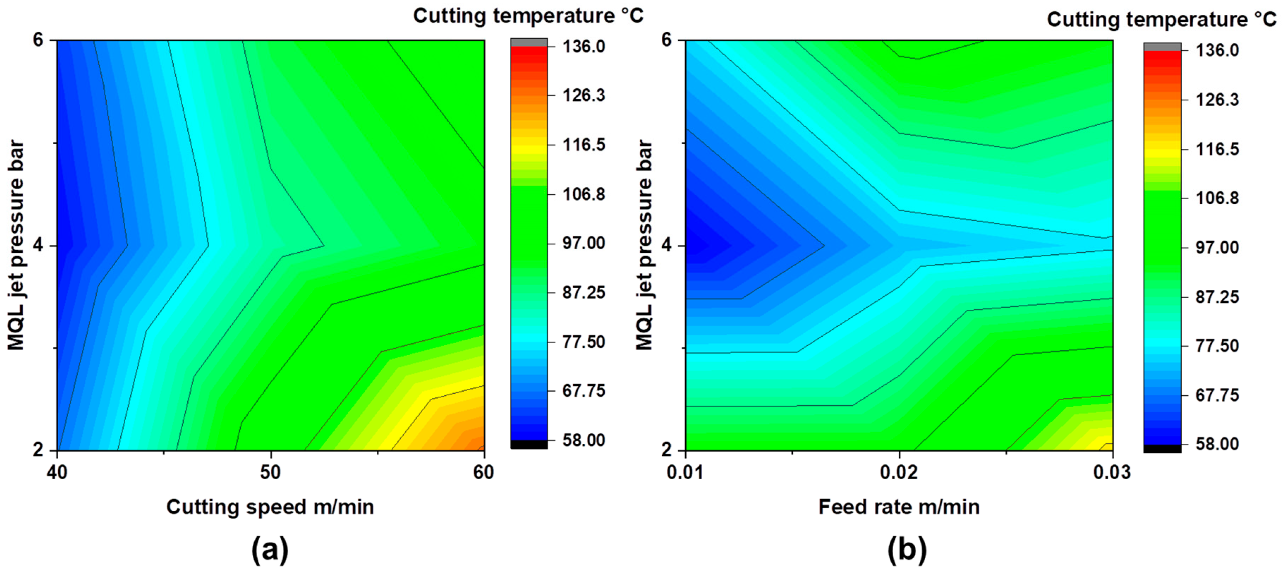
Examining Tc is essential, as it reveals how heat is generated and distributed in machining, influencing tool life and workpiece accuracy. This knowledge aids in selecting suitable cutting parameters, cooling methods, and tool materials to enhance efficiency and reliability [52]. Figure 3a depicts the effect of three different Vc at varying Pj on Tc. It is observed that increasing the Pj generally reduces the Tc, while higher Vc leads to a substantial rise in Tc. This increase is attributed to the higher relative velocity between the tool and workpiece, which intensifies frictional heating at the cutting zone. Furthermore, elevated Vc intensifies plastic deformation in the workpiece material, thereby increasing thermal accumulation [53].
Higher Pj improves the cooling and lubrication effectiveness at the interface between the tool and workpiece. At low pressures, such as 2 bar, the mist does not penetrate efficiently into the cutting zone, allowing heat to accumulate and resulting in higher Tc [54]. Conversely, at excessively high pressures, such as 6 bar, the air pressure induces a spring-back effect, causing droplets to rebound from the cutting surface and reducing the effectiveness of lubrication. Thus, both very low and excessively high Pj can lead to elevated Tc. Optimal Pj provides sufficient penetration and heat dissipation, lowering the overall Tc. At low Pj, Vc strongly dominates the thermal response, causing a steep increase in Tc, whereas at optimal Pj, the rate of Tc rise is moderated due to enhanced cooling efficiency [55].
As shown in Figure 3b, Tc also increases with higher f; however, the underlying mechanism differs from that associated with variations in Vc, reflecting the distinct ways in which f influences the rise in Tc in the cutting zone. Higher f increases the uncut chip thickness, generating larger Fc and greater plastic deformation in the shear zone, which intensifies heat generation due to elevated shear strain and tool–chip friction [56]. Pj similarly regulates the thermal response under varying f. At low Pj, insufficient heat evacuation leads to thermal accumulation, whereas optimal Pj improves atomization and cooling, reducing the effective Tc. The interaction between f and Pj indicates that the adverse effect of higher f can be partially mitigated by increasing the Pj. Adequate Pj ensures that Tc remains within acceptable limits, even at higher f. This occurs because higher f generates more frictional heat, while an optimum Pj enhances coolant penetration, lubrication, and chip evacuation. Consequently, the additional heat is effectively dissipated, keeping Tc within controlled thermal boundaries even at elevated f levels [57]. From the contour plot analysis, the minimum Tc of 58 °C was achieved at a Vc of 40 m/min, f of 0.01 mm/rev, and Pj of 4 bar. Conversely, the maximum Tc of 136 °C occurred at 60 m/min Vc, 0.01 mm/rev f, and 2 bar Pj. Therefore, under the CMQL lubricating environment, the optimal cutting condition for minimizing Tc was identified as a Vc of 40 m/min, f of 0.01 mm/rev, and Pj of 4 bar.
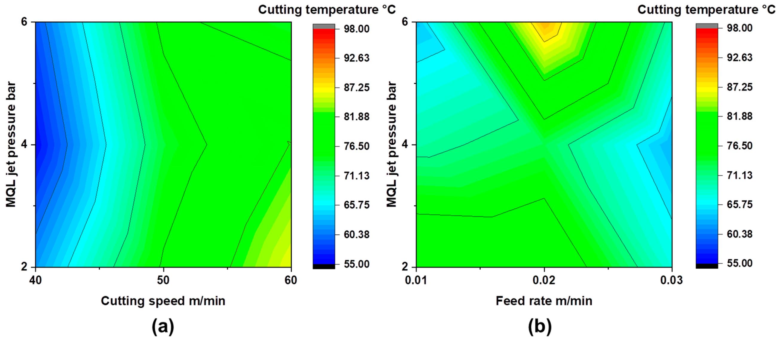
The contour plot in Figure 4 demonstrates how Tc responds to variations in machining parameters under a GEMQL environment. Specifically, Figure 4a highlights the relationship between Vc and Pj, showing their combined impact on the temperature generated during the cutting process. The GEMQL lubricating environment significantly reduces Tc across all machining conditions compared to the CMQL environment. This improvement is primarily attributed to the enhanced lubrication properties provided by Gnps, which improve the fluid’s thermal stability, retainability in the cutting zone, and the formation of a protective tribo-film on the tool–workpiece interface [58]. At lower Pj, such as 2 bar in the CMQL setup, the cooling effect is insufficient; however, the presence of Gnps in GEMQL compensates for this limitation by promoting effective heat dissipation and reducing friction. Similarly, the spring-back effect observed at 6 bar MQL pressure under CMQL conditions is mitigated in GEMQL due to the rolling action of Gnps, which facilitates smoother tool–chip interaction and further decreases Tc in this high-pressure region [59].
As illustrated in Figure 4b, lower Tc values are achieved at both higher and lower feed rate ranges. The maximum Tc recorded was 98 °C at a Vc of 60 m/min, a f of 0.02 mm/rev, and 2 bar Pj. While this temperature is elevated under these conditions, it remains lower than the corresponding CMQL condition, which reached 106 °C. The maximum reduction in Tc of 36.8% was observed in the GEMQL environment compared to the CMQL environment at a Vc of 60 m/min, a f of 0.01 mm/rev, and a Pj of 2 bar. Similarly, Danush et al. reported a 31% reduction in Tc while milling Inconel 718 using a Gnps-based sunflower oil MQL system [60]. Analysis of the contour plots indicates that the optimal cutting conditions in the GEMQL environment are a Vc of 40 m/min, a f of 0.03 mm/rev, and a Pj of 4 bar.

3.2. Insight into Data Processing

Effective data processing plays a pivotal role in ML by converting raw data into informative representations that maximize a model’s predictive capability. The distribution plot presented in Figure 5 illustrates the spread of the independent variables, namely Vc, f, and Pj. The Vc values considered in the dataset are 40 m/min, 50 m/min, and 60 m/min, while the f values are 0.01 mm/rev, 0.02 mm/rev, and 0.03 mm/rev. In a similar manner, the Pj values are 2 bar, 4 bar, and 6 bar. These independent variables are uniformly distributed, ensuring that the dataset provides an unbiased representation of the selected ranges.
In contrast, the dependent variable, Tc, exhibits noticeable skewness, indicating that its distribution is not symmetric. This skewness arises due to the presence of two distinct lubricating conditions, namely CMQL and GEMQL, which influence the temperature distribution differently under varying cutting parameters. To further assess the data quality, outlier analysis was performed using violin plots, as shown in Figure 6. The analysis revealed that no significant outliers were present in either the independent or dependent variables, thereby confirming the reliability of the experimental dataset. The absence of outliers is crucial, as extreme values can skew model training and lead to biased predictions, reducing overall accuracy.
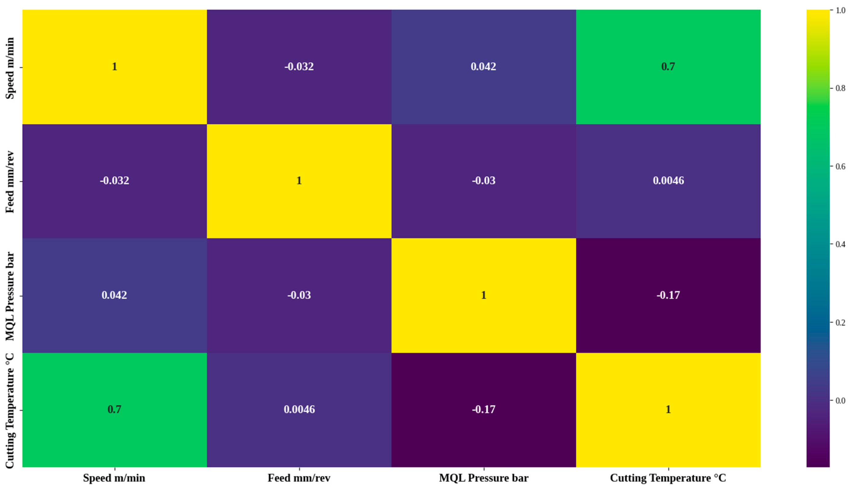
The correlation analysis between the dependent variable (Tc) and the independent variables is illustrated in Figure 7, as examining these relationships helps identify influential features and improves model performance. The results demonstrate that Tc has the strongest positive correlation (0.7) with Vc, suggesting that an increase in Vc significantly elevates the Tc. A very weak positive correlation (0.033) was observed between Tc and f, implying that the effect of f on Tc is minimal. On the other hand, a moderate negative correlation (−0.17) was identified between Tc and Pj, indicating that higher Pj contributes to reducing the Tc to some extent.

3.3. Development and Comparison of ML Models

In this study, five advanced ML models, DT, XGBoost, KNN, RFR, and CatBoost, were initially developed as individual predictors and subsequently combined to create a hybrid stacked ML framework. In the DT model, the GridSearchCV tuning process considered three key parameters: maximum depth with values 16, 17, and 18; minimum samples per leaf with values 6, 7, and 8; and minimum samples per split with values 1, 2, and 4. The cross-validation was performed with three folds to ensure the reliability of the results. Maximum depth controls the overall complexity of the tree, while minimum samples per leaf regulates the minimum number of observations at the terminal nodes, preventing overly specific rules. Similarly, a minimum sample per split ensures that a node must have a sufficient number of samples before it can be divided further, thereby improving generalization. Based on this process, the optimal combination of hyperparameters was identified as max_depth = 17, min_samples_leaf = 8, and min_samples_split = 2. The performance of the tuned model was assessed using negative mean squared error (NMSE), which yielded a value of –91.48, demonstrating the effectiveness of parameter optimization in improving model accuracy.
The XGBoost model was tuned using five-fold cross-validation to identify the optimal hyperparameter. The values explored in the search included maximum depth with values [3, 5, 7, 10], number of estimators with values [50, 100, 200], learning rate with values [0.01, 0.05, 0.1, 0.2], subsample with values [0.7, 0.8, 1.0], and column sample by tree with values [0.7, 0.8, 1.0]. Based on this comprehensive search, the best parameters identified were a maximum depth of five, a learning rate of 0.1, a number of estimators was 200, a subsample value of 0.7, and a column sample by tree value of 1.0.
In the KNN model, the similarity between data points was measured using a distance metric, and the outcome was determined based on either equal weighting or distance-based weighting of the neighbors. The parameter “grid” explored included the number of neighbors with values [3, 5, 7, 9, 11], the weighting scheme with options “uniform” and “distance,” and the distance metric with options “Euclidean” and “Manhattan.” The grid search systematically evaluated all parameter combinations using two-fold validation, with performance measured through negative mean squared error. From this optimization process, the best parameters were identified as a distance metric of Manhattan, a number of neighbors equal to three, and a weighting scheme of distance. This configuration achieved an NMSE of −69.94.
The RFR model parameter “grid” was designed to explore different combinations of key hyperparameters. The parameter “number of estimators” was tested with values [50, 100, 200], which determines how many decision trees are included in the forest. The parameter “maximum depth” was set to [5, 10, 20] to control how deep each tree could grow, balancing model complexity with generalization. The parameter “minimum samples split with values” [2, 5, 10] specifies the least number of samples required to divide an internal node, while “minimum samples leaf with values” [1, 2, 4] determines the smallest number of samples allowed in a leaf node. These parameters play a key role in preventing overfitting and enhancing the model’s stability. After the extensive search of GridSearchCV, the optimal configuration was determined to be a maximum depth of 20, 1 sample per leaf, 5 samples required to split a node, and 200 estimators. The optimized model achieved the best score of NMSE as −69.74.
The parameter “grid” for the CatBoost model was formulated to investigate various values of three key hyperparameters. The learning rate was tested with values [0.1, 0.2, 0.3], which controls the step size at each boosting iteration and balances the trade-off between speed of learning and overfitting. The depth was varied across [6, 8, 10], representing the maximum depth of the decision trees that form the base learners, with deeper trees allowing the model to capture more complexity. The iterations were set to [100, 200, 300], which determines the total number of boosting rounds and directly impacts how many trees are built in the ensemble. The best parameter set identified through hyperparameter tuning was a depth of 8, number of iterations equal to 300, and a learning rate of 0.1. The tuned model achieved a best score of −64.23, which represents an improvement in minimizing prediction error compared to other tested configurations.
The modeling section of HSMLM introduces a diverse set of base learners whose hyperparameters were selected based on the best-performing configurations obtained through GridSearchCV for each individual model. The KNN regressor predicts values by averaging the outcomes of the five closest neighbors (n_neighbors = 5). The DT algorithm is restricted to a maximum depth of ten (max_depth = 10) to avoid overfitting, while the RFR consists of 400 trees (n_estimators = 400), each trained on random subsets of the data to enhance robustness. The XGBoost model applies gradient boosting with 600 boosting rounds (n_estimators = 600), a conservative learning rate of 0.03 to ensure gradual updates, and a maximum tree depth of six (max_depth = 6), while incorporating subsampling (subsample = 0.9) and column sampling (colsample_bytree = 0.9) to improve generalization. The CatBoost is optimized with 1200 boosting iterations, a tree depth of eight, and a learning rate of 0.03, along with an l2_leaf_reg = 6.0 regularization term to control complexity and reduce overfitting.
To combine the strengths of these models, a Stacking Regressor is employed, where the predictions of the base models are passed to a meta-learner. The chosen meta-model is an ElasticNetCV, a linear regression method that applies both L1 and L2 regularization. The parameter l1_ratio = [0.1, 0.5, 0.9] specifies different balances between L1 and L2 penalties, while alphas = np.logspace(−4, 1, 12) tests a range of penalty strengths. Cross-validation with five folds (cv = 5) ensures that the best set of hyperparameters is selected. Additionally, the passthrough = True argument ensures that the meta-model not only sees the predictions of the base models but also the original features, enriching the final prediction process.
Finally, the complete modeling workflow is wrapped in a pipeline, which integrates preprocessing and stacking into a single object. To address skewness in the target variable, the model is trained inside a Transformed Target Regressor that applies a Yeo–Johnson power transformation, making the target distribution more symmetric and thus easier for the models to learn. The fit method at the end trains the pipeline end-to-end, so that preprocessing, base model training, stacking, and target transformation are executed in a seamless and unified manner.
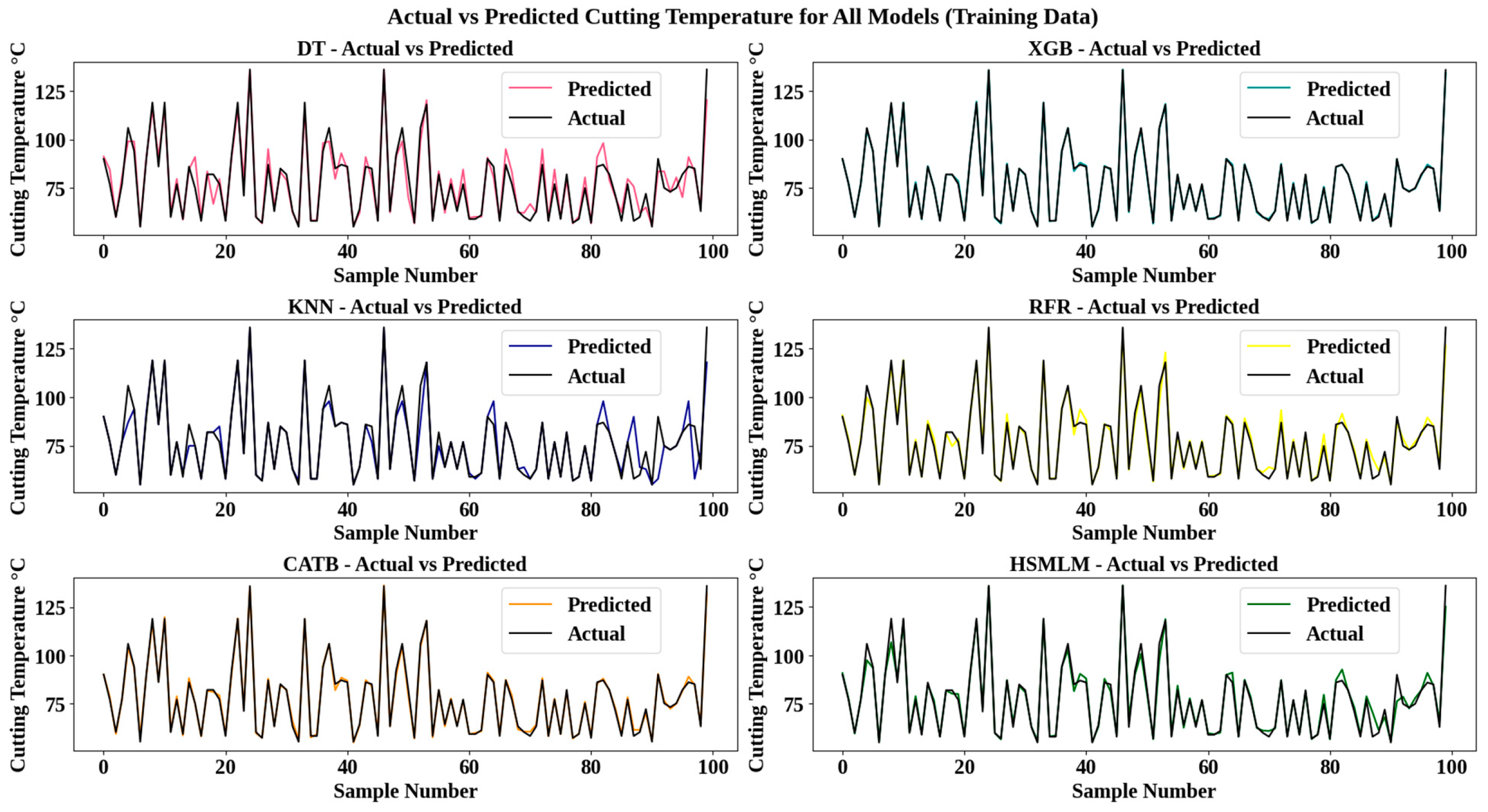
In the constructed models DT, XGBoost, KNN, RFR, CatBoost and HSMLM, each showed strong learning ability on the training dataset, producing low error values and high accuracy. Their performance on the training data is illustrated in Figure 8. However, the true reliability of a model is best determined by how it performs on the test dataset. Test data results act as the key benchmark, showing how effectively the models can uncover real patterns and provide accurate predictions for unseen cases. Therefore, this study places greater importance on test data performance, as it more clearly reflects the models’ generalization ability and practical usefulness.
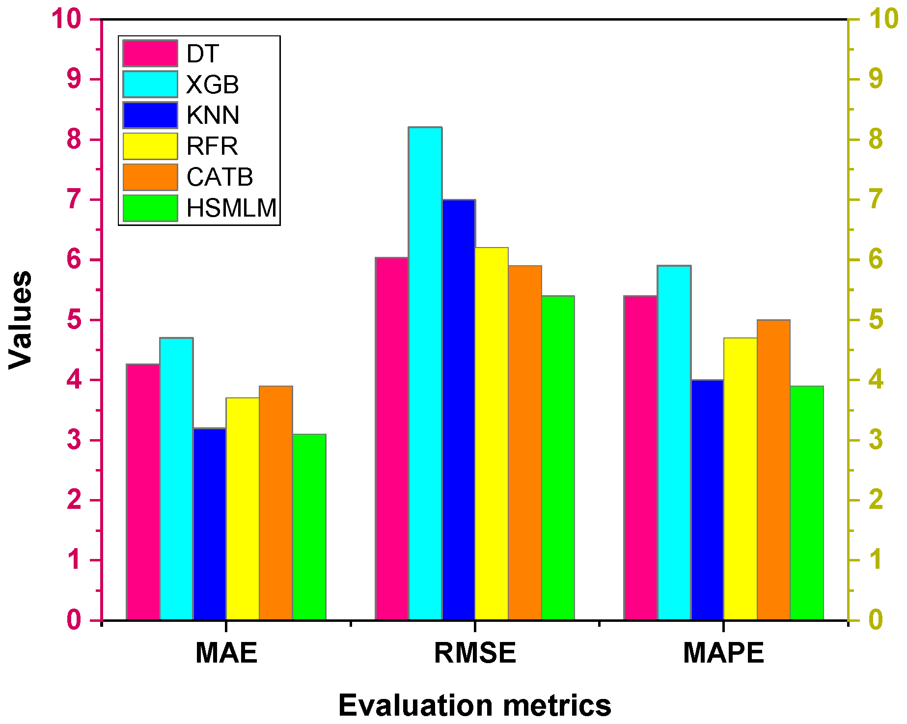
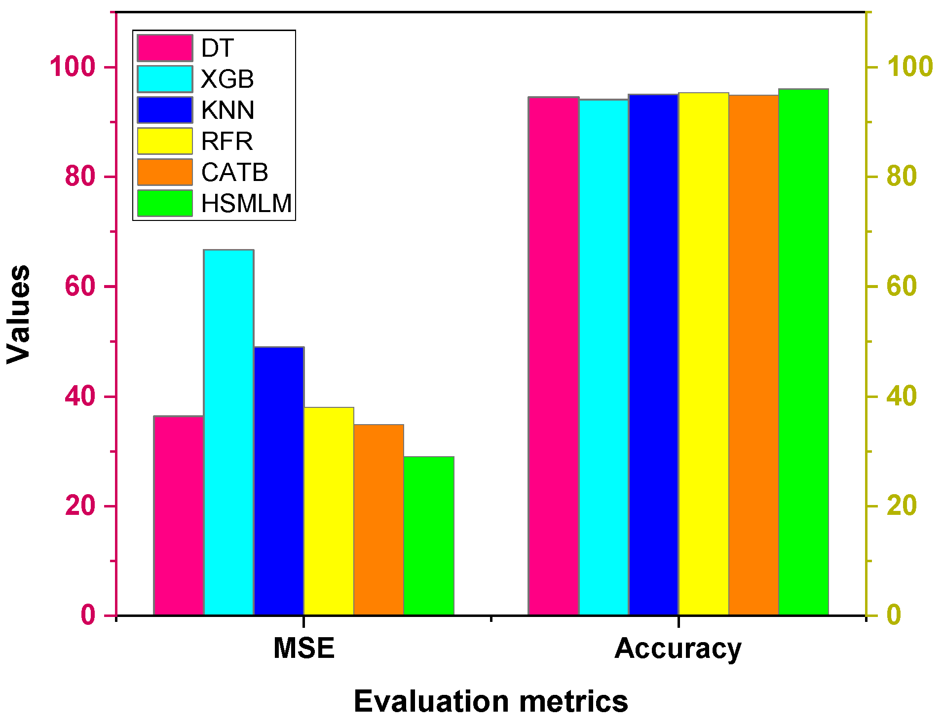
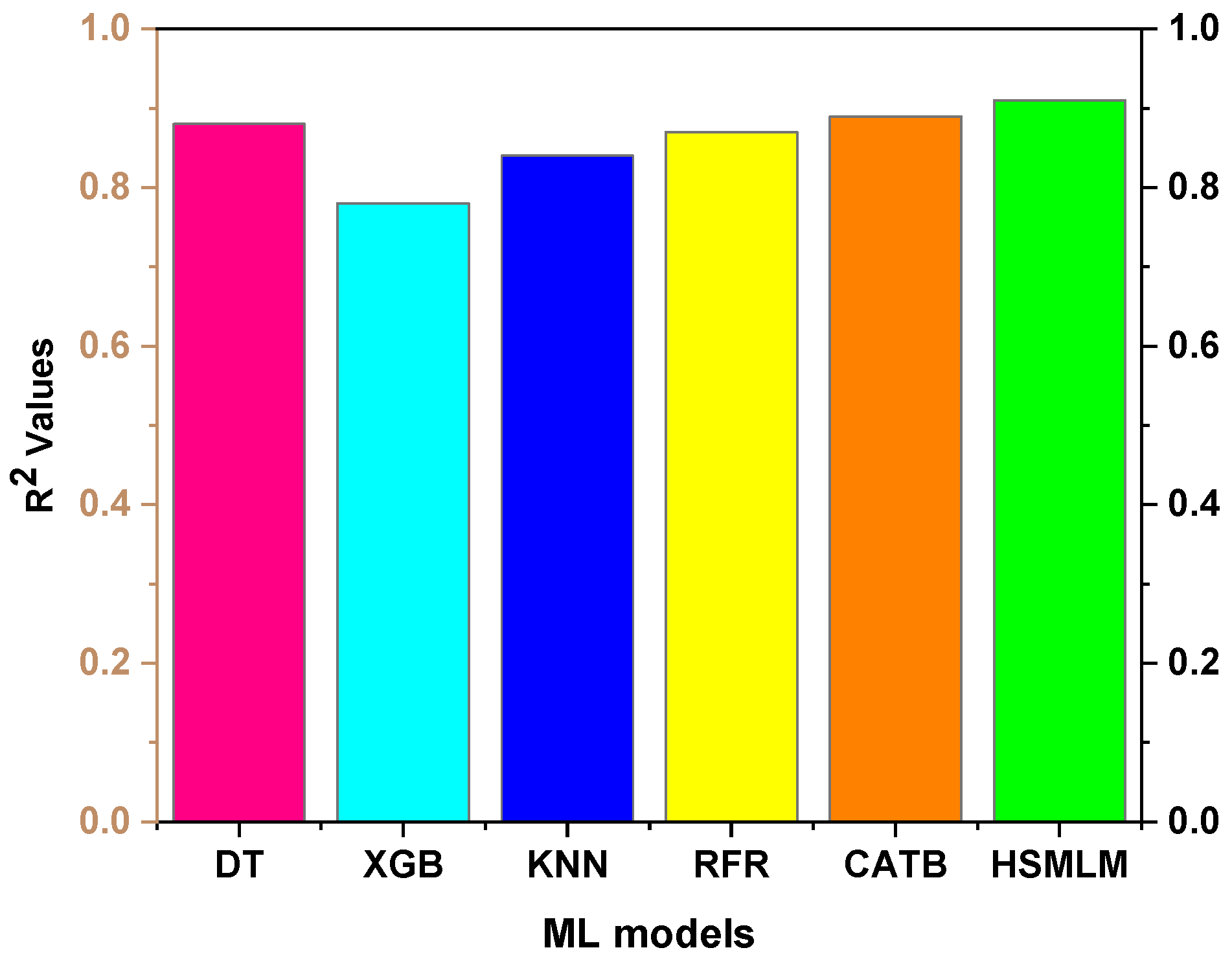
The prediction performance of all ML models on the testing dataset was evaluated using multiple statistical metrics. MAE, RMSE, and MAPE are presented in Figure 9, MSE and Accuracy in Figure 10, and R2 in Figure 11. The DT model demonstrated reliable predictive capability, achieving an MAE of 4.26, an RMSE of 6.04, an MAPE of 5.4, an MSE of 36.4, an accuracy of 94.5%, and an R2 of 0.88. Its relatively strong performance can be attributed to its ability to capture non-linear relationships and interactions between input features efficiently, allowing it to model complex patterns in the data [61]. However, despite these strengths, the relatively simple tree structure may still limit its generalization ability in certain cases.
The KNN model produced lower MAE (3.2) and MAPE (4.0) compared with DT, indicating stronger local prediction accuracy. However, its RMSE (7.0) and MSE (49) were higher, reflecting sensitivity to data variability. The accuracy (95%) was comparable to DT, while the R2 value (0.84) was slightly lower, indicating reduced overall explanatory power. The comparatively lower performance in terms of global error metrics can be attributed to KNN’s reliance on local neighbors, which makes it sensitive to fluctuations in the data and less effective at capturing overall trends across the entire dataset [62].
The RFR achieved an MAE of 3.7, an RMSE of 6.2, an MAPE of 4.7, an MSE of 38, an accuracy of 95.3%, and an R2 of 0.87. Its high performance is due to the ensemble design, which aggregates multiple decision trees to lower variance and enhance robustness while keeping bias at a moderate level. This allows RFR to capture patterns more effectively than individual trees and generalize well across the dataset [63]. The CatBoost model outperformed RFR in terms of RMSE (5.9), MSE (34.8), and R2 (0.89), demonstrating superior capability in modeling complex non-linear relationships and interactions within the data. However, MAE (3.9), MAPE (5.0), and accuracy (94.9%) were slightly lower, which may be due to the algorithm’s sensitivity to certain localized variations in the dataset and its reliance on gradient boosting iterations [64], making it occasionally less robust to small fluctuations compared with RFR.
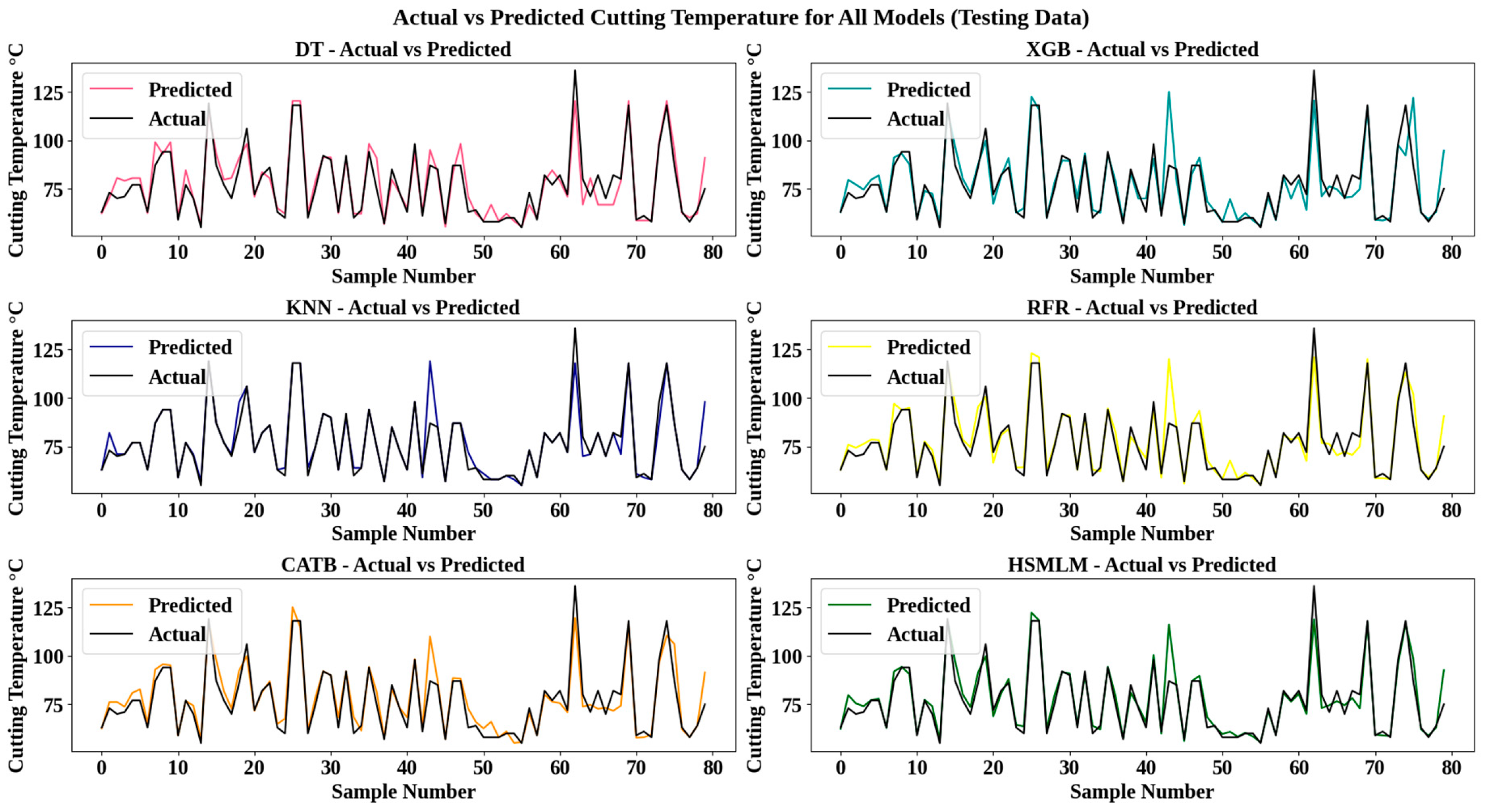
The XGBoost model showed the lowest performance among all models, with a MAE of 4.7, RMSE of 8.2, MAPE of 5.9, MSE of 66.7, accuracy of 94.1%, and R2 of 0.78. The reduced performance can be attributed to its sensitivity to hyperparameter settings and higher variance, which may limit its ability to generalize effectively on the test dataset, particularly in regions with complex or sparse data patterns [65]. The proposed HSMLM achieved the best performance, with an MAE of 3.1, an RMSE of 5.4, an MAPE of 3.9, an MSE of 29, an accuracy of 96%, and an R2 of 0.91. Its superior performance can be attributed to the ensemble stacking approach, which effectively combines the strengths of individual base models, reducing both bias and variance, and enhancing predictive robustness and generalization to unseen data. Correspondingly, Zeng et al. reported strong predictive capability using a physics-informed meta-learning model, achieving an R2 of 0.89 and MAPE of 12.33 for surface roughness prediction in the milling of S45C steel [66]. Figure 12 presents a comparison of the predictive performance of all six models evaluated on the testing dataset.

4. Conclusions

This study examines the effect of Gnps-enhanced sesame oil in an MQL system during the milling of H11 hot die steel. An HSMLM model was devised to predict cutting temperature, and its performance was compared with base learners, including DT, XGBoost, KNN, RFR, and CatBoost. The following conclusions are drawn:
The GEMQL environment notably lowers Tc compared to CMQL, due to Gnps-enhanced lubrication that improves thermal stability, fluid retention, and protective tribo-film formation at the tool–workpiece interface.
The lowest Tc of 58 °C in the CMQL environment was observed at a Vc of 40 m/min, a f of 0.01 mm/rev, and a Pj of 4 bar.
The GEMQL environment achieved a maximum Tc reduction of 36.8% compared to CMQL at a Vc of 60 m/min, a f of 0.01 mm/rev, and a Pj of 2 bar. This reduction surpasses the result reported in the existing study employing Gnps-enhanced sunflower oil under MQL milling.
Under the optimum parameters of 40 m/min Vc, 0.03 mm/rev f, and 4 bar Pj, GEMQL achieves the lowest Tc of 55 °C, significantly lower than CMQL.
Among the six ML models, XGBoost showed the lowest performance (MAE: 4.7, RMSE: 8.2, MAPE: 5.9, MSE: 66.7, accuracy: 94.1%, R2: 0.78) due to its sensitivity to hyperparameters and higher variance, limiting generalization on sparse test data.
The proposed HSMLM achieved the highest performance with an MAE of 3.1, an RMSE of 5.4, an MAPE of 3.9, an MSE of 29, an accuracy of 96%, and an R2 of 0.91, as its ensemble stacking effectively combines base models to enhance accuracy, robustness, and generalization. It also performs better than the existing physics-informed meta-learning approach reported for surface roughness prediction.

Author Contributions

Conceptualization, S.A.; Methodology, T.K.S.; Formal analysis, B.A.; Investigation, B.A.; Resources, T.K.S.; Data curation, T.K.S.; Writing—original draft, B.A.; Writing—review & editing, S.A.; Visualization, S.A.; Supervision, S.A. All authors have read and agreed to the published version of the manuscript.

Funding

This research received no external funding.

Data Availability Statement

The original contributions presented in the study are included in the article, further inquiries can be directed to the corresponding author.

Conflicts of Interest

The authors declare no conflict of interest.

References

  1. Budzynski, P.; Kara, L.; Küçükömeroğlu, T.; Kaminski, M. The influence of nitrogen implantation on tribological properties of AISI H11 steel. Vacuum 2015, 122, 230–235. [Google Scholar] [CrossRef]
  2. Hassanpour, H.; Sadeghi, M.H.; Rasti, A.; Shajari, S. Investigation of surface roughness, microhardness and white layer thickness in hard milling of AISI 4340 using minimum quantity lubrication. J. Clean. Prod. 2016, 120, 124–134. [Google Scholar] [CrossRef]
  3. Duc, T.M.; Tuan, N.M.; Long, T.T. Optimization of Al2O3 nanoparticle concentration and cutting parameters in hard milling under nanofluid MQL environment. Adv. Mech. Eng. 2024, 16, 16878132241257114. [Google Scholar] [CrossRef]
  4. Krolczyk, G.M.; Maruda, R.W.; Krolczyk, J.B.; Wojciechowski, S.; Mia, M.; Nieslony, P.; Budzik, G. Ecological trends in machining as a key factor in sustainable production—A review. J. Clean. Prod. 2019, 218, 601–615. [Google Scholar] [CrossRef]
  5. Kazeem, R.A.; Fadare, D.A.; Ikumapayi, O.M.; Adediran, A.A.; Aliyu, S.J.; Akinlabi, S.A.; Jen, T.C.; Akinlabi, E.T. Advances in the Application of Vegetable-Oil-Based Cutting Fluids to Sustainable Machining Operations—A Review. Lubricants 2022, 10, 69. [Google Scholar] [CrossRef]
  6. Azman, N.F.; Samion, S. Dispersion Stability and Lubrication Mechanism of Nanolubricants: A Review. Int. J. Precis. Eng. Manuf. Green Technol. 2019, 6, 393–414. [Google Scholar] [CrossRef]
  7. Haq, M.A.u.; Hussain, S.; Ali, M.A.; Farooq, M.U.; Mufti, N.A.; Pruncu, C.I.; Wasim, A. Evaluating the effects of nano-fluids based MQL milling of IN718 associated to sustainable productions. J. Clean. Prod. 2021, 310, 127463. [Google Scholar] [CrossRef]
  8. Pal, A.; Chatha, S.S.; Sidhu, H.S. Performance evaluation of the minimum quantity lubrication with Al2O3- mixed vegetable-oil-based cutting fluid in drilling of AISI 321 stainless steel. J. Manuf. Process. 2021, 66, 238–249. [Google Scholar] [CrossRef]
  9. Dong, P.Q.; Duc, T.M.; Long, T.T. Performance evaluation of mqcl hard milling of skd 11 tool steel using mos2 nanofluid. Metals 2019, 9, 658. [Google Scholar] [CrossRef]
  10. Hamdi, A.; Yapan, Y.F.; Uysal, A.; Merghache, S.M. Machinability assessment and optimization of turning AISI H11 steel under various minimum quantity lubrication (MQL) conditions using nanofluids. Int. J. Adv. Manuf. Technol. 2025, 137, 4089–4107. [Google Scholar] [CrossRef]
  11. Taghvaei, M.; Jafari, S.M. Application and stability of natural antioxidants in edible oils in order to substitute synthetic additives. J. Food Sci. Technol. 2015, 52, 1272–1282. [Google Scholar] [CrossRef]
  12. Padmini, R.; Vamsi Krishna, P.; Krishna Mohana Rao, G. Performance assessment of micro and nano solid lubricant suspensions in vegetable oils during machining. Proc. Inst. Mech. Eng. Part B J. Eng. Manuf. 2015, 229, 2196–2204. [Google Scholar] [CrossRef]
  13. Ni, J.; Cui, Z.; Wu, C.; Sun, J.; Zhou, J. Evaluation of MQL broaching AISI 1045 steel with sesame oil containing nano-particles under best concentration. J. Clean. Prod. 2021, 320, 128888. [Google Scholar] [CrossRef]
  14. Phiri, J.; Gane, P.; Maloney, T.C. General overview of graphene: Production, properties and application in polymer composites. Mater. Sci. Eng. B 2017, 215, 9–28. [Google Scholar] [CrossRef]
  15. Hou, X.; Xie, Z.; Li, C.; Li, G.; Chen, Z. Study of electronic structure, thermal conductivity, elastic and optical properties of α, β, γ-graphyne. Materials 2018, 11, 188. [Google Scholar] [CrossRef]
  16. Touggui, Y.; Uysal, A.; Emiroglu, U.; Belhadi, S.; Temmar, M. Evaluation of MQL performances using various nanofluids in turning of AISI 304 stainless steel. Int. J. Adv. Manuf. Technol. 2021, 115, 3983–3997. [Google Scholar] [CrossRef]
  17. de Paiva, R.L.; de Oliveira, D.; Ruzzi, R.d.S.; Jackson, M.J.; Gelamo, R.V.; Abrão, A.M.; da Silva, R.B. Surface roughness and morphology evaluation of bearing steel after grinding with multilayer graphene platelets dispersed in different base fluids. Wear 2023, 523, 204852. [Google Scholar] [CrossRef]
  18. Pal, A.; Singh, S.; Singh, H. Tribology International Experimental investigation on the performance of MQL drilling of AISI 321 stainless steel using nano-graphene enhanced vegetable-oil-based cutting fluid. Tribol. Int. 2020, 151, 106508. [Google Scholar] [CrossRef]
  19. Jiang, J.; Wu, Z.; Pan, S.; Meng, X.; Liu, D.; Mu, K.; Zhu, Q.; Zhu, J.; Cai, C. High-performance liquid metal-based SiC/Graphene-Mo hybrid nanofluid for hydraulic transmission. Tribol. Int. 2024, 198, 109871. [Google Scholar] [CrossRef]
  20. Li, M.; Li, Q.; Pan, X.; Wang, J.; Wang, Z.; Xu, S.; Zhou, Y.; Ma, L.; Yu, T. On understanding milling characteristics of TC4 alloy during graphene nanofluid minimum quantity lubrication with bionic micro-texture tool. J. Mater. Res. Technol. 2025, 36, 4200–4214. [Google Scholar] [CrossRef]
  21. Fisher, O.J.; Watson, N.J.; Porcu, L.; Bacon, D.; Rigley, M.; Gomes, R.L. Multiple target data-driven models to enable sustainable process manufacturing: An industrial bioprocess case study. J. Clean. Prod. 2021, 296, 126242. [Google Scholar] [CrossRef]
  22. Mia, M.; Dhar, N.R. Response surface and neural network based predictive models of cutting temperature in hard turning. J. Adv. Res. 2016, 7, 1035–1044. [Google Scholar] [CrossRef]
  23. Gupta, M.K.; Mia, M.; Pruncu, C.I.; Khan, A.M.; Rahman, M.A.; Jamil, M.; Sharma, V.S. Modeling and performance evaluation of Al2O3, MoS2 and graphite nanoparticle-assisted MQL in turning titanium alloy: An intelligent approach. J. Braz. Soc. Mech. Sci. Eng. 2020, 42, 207. [Google Scholar] [CrossRef]
  24. Zhang, Y.; Xu, X. Machine learning cutting force, surface roughness, and tool life in high speed turning processes. Manuf. Lett. 2021, 29, 84–89. [Google Scholar] [CrossRef]
  25. Jurkovic, Z.; Cukor, G.; Brezocnik, M.; Brajkovic, T. A comparison of machine learning methods for cutting parameters prediction in high speed turning process. J. Intell. Manuf. 2018, 29, 1683–1693. [Google Scholar] [CrossRef]
  26. Abu-Mahfouz, I.; El Ariss, O.; Esfakur Rahman, A.H.M.; Banerjee, A. Surface roughness prediction as a classification problem using support vector machine. Int. J. Adv. Manuf. Technol. 2017, 92, 803–815. [Google Scholar] [CrossRef]
  27. Sizemore, N.E.; Nogueira, M.L.; Greis, N.P.; Davies, M.A. Application of machine learning to the prediction of surface roughness in diamond machining. Procedia Manuf. 2020, 48, 1029–1040. [Google Scholar] [CrossRef]
  28. Azevedo, B.F.; Rocha, A.M.A.C.; Pereira, A.I. Hybrid Approaches to Optimization and Machine Learning Methods: A Systematic Literature Review. Mach. Learn. 2024, 113, 4055–4097. [Google Scholar] [CrossRef]
  29. Ostad Ali Akbari, V.; Kuffa, M.; Wegener, K. Physics-informed Bayesian machine learning for probabilistic inference and refinement of milling stability predictions. CIRP J. Manuf. Sci. Technol. 2023, 45, 225–239. [Google Scholar] [CrossRef]
  30. Rahman, M.W.; Zhao, B.; Pan, S.; Qu, Y. Microstructure-informed machine learning for understanding corrosion resistance in structural alloys through fusion with experimental studies. Comput. Mater. Sci. 2025, 248, 113624. [Google Scholar] [CrossRef]
  31. Kim, G.; Yang, S.M.; Kim, D.M.; Kim, S.; Choi, J.G.; Ku, M.; Lim, S.; Park, H.W. Bayesian-based uncertainty-aware tool-wear prediction model in end-milling process of titanium alloy. Appl. Soft Comput. 2023, 148, 110922. [Google Scholar] [CrossRef]
  32. Huang, Z.; Shao, J.; Guo, W.; Li, W.; Zhu, J.; Fang, D. Hybrid machine learning-enabled multi-information fusion for indirect measurement of tool flank wear in milling. Meas. J. Int. Meas. Confed. 2023, 206, 112255. [Google Scholar] [CrossRef]
  33. Karmi, Y.; Boumediri, H.; Reffas, O.; Chetbani, Y.; Ataya, S.; Khan, R.; Yallese, M.A.; Laouissi, A. Integration of Hybrid Machine Learning and Multi-Objective Optimization for Enhanced Turning Parameters of EN-GJL-250 Cast Iron. Crystals 2025, 15, 264. [Google Scholar] [CrossRef]
  34. Zhang, S.; Ding, T.C.; Li, J.F. Microstructural alteration and microhardness at near-surface of aisi H13 steel by Hard Milling. Mach. Sci. Technol. 2012, 16, 473–486. [Google Scholar] [CrossRef]
  35. Balasuadhakar, A.; Thirumalai Kumaran, S.; Uthayakumar, M. Machine learning prediction of surface roughness in sustainable machining of AISI H11 tool steel. Smart Mater. Manuf. 2025, 3, 100075. [Google Scholar] [CrossRef]
  36. Al-Janabi, A.S.; Hussin, M.; Abdullah, M.Z. Stability, thermal conductivity and rheological properties of graphene and MWCNT in nanolubricant using additive surfactants. Case Stud. Therm. Eng. 2021, 28, 101607. [Google Scholar] [CrossRef]
  37. Peng, R.; Liu, J.; Chen, M.; Tong, J.; Zhao, L. Development of a pressurized internal cooling milling cutter and its machining performance assessment. Precis. Eng. 2021, 72, 315–329. [Google Scholar] [CrossRef]
  38. Rohit, J.N.; Surendra Kumar, K.; Sura Reddy, N.; Kuppan, P.; Balan, A.S.S. Computational Fluid Dynamics Analysis of MQL Spray Parameters and Its Influence on MQL Milling of SS304. In Simulations for Design and Manufacturing; Lecture Notes on Multidisciplinary Industrial Engineering; Springer: Singapore, 2018; pp. 45–78. ISBN 9789811085185. [Google Scholar]
  39. Samy, G.S.; Thirumalai Kumaran, S.; Uthayakumar, M. An analysis of end milling performance on B4C particle reinforced aluminum composite. J. Aust. Ceram. Soc. 2017, 53, 373–383. [Google Scholar] [CrossRef]
  40. Dewes, R.C.; Ng, E.; Chua, K.S.; Newton, P.G.; Aspinwall, D.K. Temperature measurement when high speed machining hardened mould/die steel. J. Mater. Process. Technol. 1999, 92–93, 293–301. [Google Scholar] [CrossRef]
  41. Qian, S.; Peng, T.; Tao, Z.; Li, X.; Nazir, M.S.; Zhang, C. An evolutionary deep learning model based on XGBoost feature selection and Gaussian data augmentation for AQI prediction. Process Saf. Environ. Prot. 2024, 191, 836–851. [Google Scholar] [CrossRef]
  42. Patgiri, R.; Katari, H.; Kumar, R.; Sharma, D. Empirical Study on Malicious URL Detection Using Machine Learning. In Distributed Computing and Internet Technology, Proceedings of the 15th International Conference, ICDCIT 2019, Bhubaneswar, India, 10–13 January 2019; Lecture Notes in Computer Science (Including Subseries Lecture Notes in Artificial Intelligence and Lecture Notes in Bioinformatics); Springer International Publishing: Berlin/Heidelberg, Germany, 2019; Volume 11319, pp. 380–388. [Google Scholar] [CrossRef]
  43. Rodríguez, J.J.; Quintana, G.; Bustillo, A.; Ciurana, J. A decision-making tool based on decision trees for roughness prediction in face milling. Int. J. Comput. Integr. Manuf. 2017, 30, 943–957. [Google Scholar] [CrossRef]
  44. Abedi, R.; Costache, R.; Shafizadeh-Moghadam, H.; Pham, Q.B. Flash-flood susceptibility mapping based on XGBoost, random forest and boosted regression trees. Geocarto Int. 2022, 37, 5479–5496. [Google Scholar] [CrossRef]
  45. Xiong, L.; Yao, Y. Study on an adaptive thermal comfort model with K-nearest-neighbors (KNN) algorithm. Build. Environ. 2021, 202, 108026. [Google Scholar] [CrossRef]
  46. Everingham, Y.; Sexton, J.; Skocaj, D.; Inman-Bamber, G. Accurate prediction of sugarcane yield using a random forest algorithm. Agron. Sustain. Dev. 2016, 36, 27. [Google Scholar] [CrossRef]
  47. Jabeur, S.B.; Gharib, C.; Mefteh-Wali, S.; Arfi, W. Ben CatBoost model and artificial intelligence techniques for corporate failure prediction. Technol. Forecast. Soc. Chang. 2021, 166, 120658. [Google Scholar] [CrossRef]
  48. Rtayli, N.; Enneya, N. Enhanced credit card fraud detection based on SVM-recursive feature elimination and hyper-parameters optimization. J. Inf. Secur. Appl. 2020, 55, 102596. [Google Scholar] [CrossRef]
  49. Nawa, K.; Hagiwara, K.; Nakamura, K. Prediction-accuracy improvement of neural network to ferromagnetic multilayers by Gaussian data augmentation and ensemble learning. Comput. Mater. Sci. 2023, 219, 112032. [Google Scholar] [CrossRef]
  50. Nahar, A.; Das, D. MetaLearn: Optimizing routing heuristics with a hybrid meta-learning approach in vehicular ad-hoc networks. Ad Hoc Netw. 2023, 138, 102996. [Google Scholar] [CrossRef]
  51. Nguyen-Sy, T. Optimized hybrid XGBoost-CatBoost model for enhanced prediction of concrete strength and reliability analysis using Monte Carlo simulations. Appl. Soft Comput. 2024, 167, 112490. [Google Scholar] [CrossRef]
  52. Özbek, O.; Saruhan, H. The effect of vibration and cutting zone temperature on surface roughness and tool wear in eco-friendly MQL turning of AISI D2. J. Mater. Res. Technol. 2020, 9, 2762–2772. [Google Scholar] [CrossRef]
  53. Hadad, M.J.; Tawakoli, T.; Sadeghi, M.H.; Sadeghi, B. Temperature and energy partition in minimum quantity lubrication-MQL grinding process. Int. J. Mach. Tools Manuf. 2012, 54–55, 10–17. [Google Scholar] [CrossRef]
  54. Liu, Z.Q.; Cai, X.J.; Chen, M.; An, Q.L. Investigation of cutting force and temperature of end-milling Ti-6Al-4V with different minimum quantity lubrication (MQL) parameters. Proc. Inst. Mech. Eng. Part B J. Eng. Manuf. 2011, 225, 1273–1279. [Google Scholar] [CrossRef]
  55. Zaman, P.B.; Dhar, N.R. Multi-objective Optimization of Double-Jet MQL System Parameters Meant for Enhancing the Turning Performance of Ti–6Al–4V Alloy. Arab. J. Sci. Eng. 2020, 45, 9505–9526. [Google Scholar] [CrossRef]
  56. Pal, A.; Chatha, S.S.; Singh, K. Performance evaluation of minimum quantity lubrication technique in grinding of AISI 202 stainless steel using nano-MoS2 with vegetable-based cutting fluid. Int. J. Adv. Manuf. Technol. 2020, 110, 125–137. [Google Scholar] [CrossRef]
  57. Gaitonde, V.N.; Karnik, S.R.; Davim, J.P. Selection of optimal MQL and cutting conditions for enhancing machinability in turning of brass. J. Mater. Process. Technol. 2008, 204, 459–464. [Google Scholar] [CrossRef]
  58. Peng, R.; Shen, J.; Tang, X.; Zhao, L.; Gao, J. Performances of a tailored vegetable oil-based graphene nanofluid in the MQL internal cooling milling. J. Manuf. Process. 2025, 134, 814–831. [Google Scholar] [CrossRef]
  59. dos Santos, R.G.; de Paiva, J.M.F.; Torres, R.D.; Amorim, F.L. Performance of cutting fluids with nanoparticles in the Ti5553 alloy turning process using high-speed cutting. Int. J. Adv. Manuf. Technol. 2025, 136, 4623–4645. [Google Scholar] [CrossRef]
  60. Danish, M.; Gupta, M.K.; Rubaiee, S.; Ahmed, A.; Sarikaya, M. Influence of graphene reinforced sunflower oil on thermo-physical, tribological and machining characteristics of inconel 718. J. Mater. Res. Technol. 2021, 15, 135–150. [Google Scholar] [CrossRef]
  61. Karbassi, A.; Mohebi, B.; Rezaee, S.; Lestuzzi, P. Damage prediction for regular reinforced concrete buildings using the decision tree algorithm. Comput. Struct. 2014, 130, 46–56. [Google Scholar] [CrossRef]
  62. Deng, Z.; Zhu, X.; Cheng, D.; Zong, M.; Zhang, S. Efficient kNN classification algorithm for big data. Neurocomputing 2016, 195, 143–148. [Google Scholar] [CrossRef]
  63. Johansson, U.; Boström, H.; Löfström, T.; Linusson, H. Regression conformal prediction with random forests. Mach. Learn. 2014, 97, 155–176. [Google Scholar] [CrossRef]
  64. Zhang, Y.; Ren, W.; Lei, J.; Sun, L.; Mi, Y. Case Studies in Construction Materials Predicting the compressive strength of high-performance concrete via the DR-CatBoost model. Case Stud. Constr. Mater. 2024, 21, e03990. [Google Scholar] [CrossRef]
  65. Wang, Y.; Sun, S.; Chen, X.; Zeng, X.; Kong, Y.; Chen, J.; Guo, Y.; Wang, T. Short-term load forecasting of industrial customers based on SVMD and XGBoost. Int. J. Electr. Power Energy Syst. 2021, 129, 106830. [Google Scholar] [CrossRef]
  66. Zeng, S.; Pi, D. Milling Surface Roughness Prediction Based on Physics-Informed Machine Learning. Sensors 2023, 23, 4969. [Google Scholar] [CrossRef]
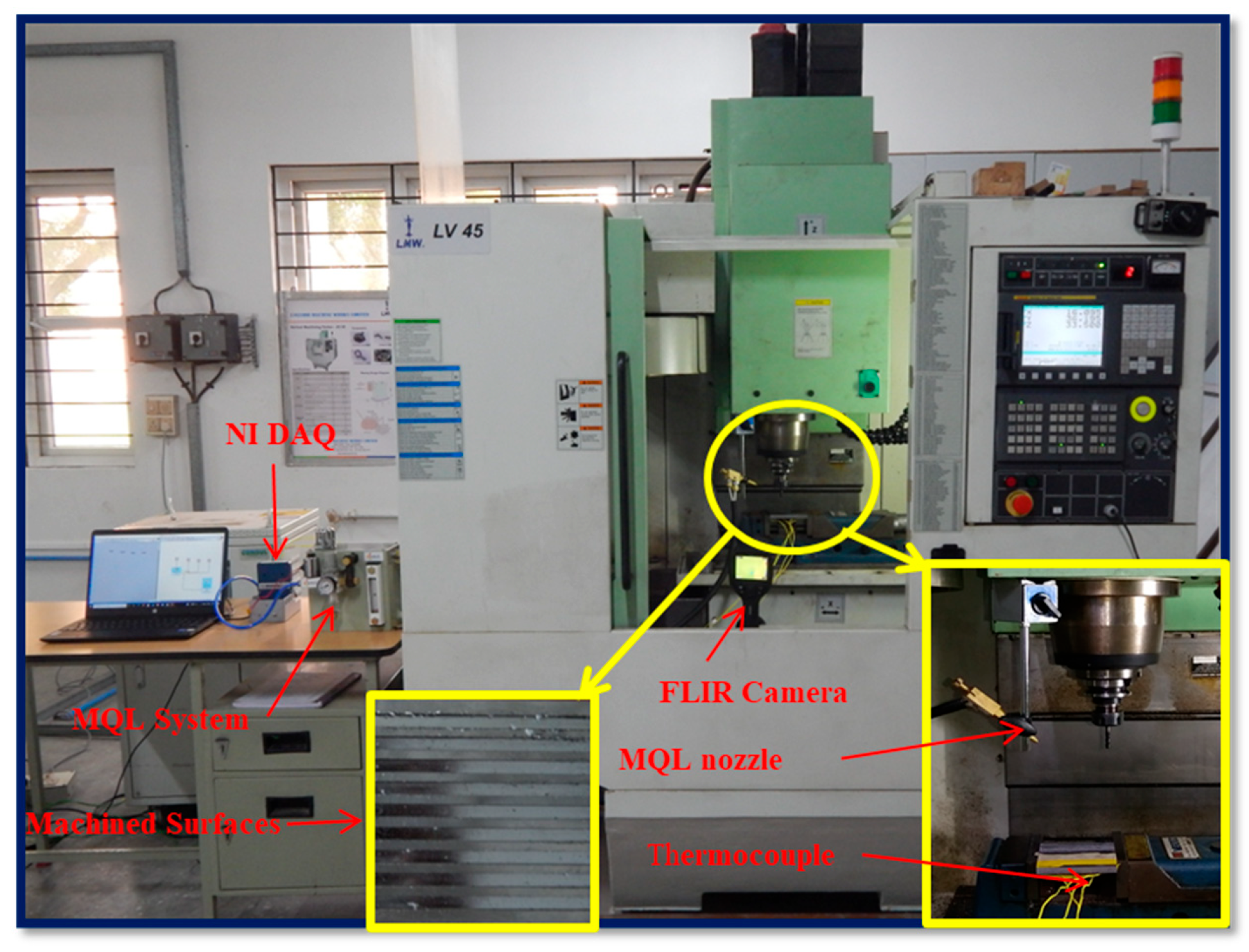
Figure 1. Experimental setup.
Lubricants 13 00498 g001
Figure 2. HSMLM Algorithm.
Lubricants 13 00498 g002
Figure 3. Tc at CMQL environment (a) Vc vs. Pj (b) f vs. P.
Lubricants 13 00498 g003
Figure 4. Tc at GEMQL environment (a) Vc vs. Pj (b) f vs. P.
Lubricants 13 00498 g004
Figure 5. Distribution of independent and dependent variables.
Lubricants 13 00498 g005
Figure 6. Violin plot for outlier detection.
Lubricants 13 00498 g006
Figure 7. Correlation heat map.
Lubricants 13 00498 g007
Figure 8. Predictive performances of models with training data.
Lubricants 13 00498 g008
Figure 9. MAE, RMSE and MAPE of ML models.
Lubricants 13 00498 g009
Figure 10. MSE and Accuracy of ML models.
Lubricants 13 00498 g010
Figure 11. R2 values of ML models.
Lubricants 13 00498 g011
Figure 12. Predictive performances of models with testing data.
Lubricants 13 00498 g012
Disclaimer/Publisher’s Note: The statements, opinions and data contained in all publications are solely those of the individual author(s) and contributor(s) and not of MDPI and/or the editor(s). MDPI and/or the editor(s) disclaim responsibility for any injury to people or property resulting from any ideas, methods, instructions or products referred to in the content.