Abstract
Ball joints are components of the vehicle axle, and their friction characteristics must be considered when evaluating vibration behavior and ride comfort in driving simulator-based simulations. To model the three-dimensional friction behavior of ball joints, real-time capability and intuitive parameterization using data from standardized component test benches are essential. These requirements favor phenomenological modeling approaches. This paper applies a spherical, three-dimensional friction model based on the LuGre model, compares it with alternative approaches, and introduces a universal parameter estimation framework using machine learning. Furthermore, the kinematic operating ranges of ball joints are derived from vehicle measurements, and component-level measurements are conducted accordingly. The collected measurement data are used to estimate model parameters through gradient-based optimization for all considered models. The results of the model fitting are presented, and the model characteristics are discussed in the context of their suitability for online simulation in a driving simulator environment. We demonstrate that the proposed parameter estimation framework is capable of learning all the applied models. Moreover, the three-dimensional LuGre-based approach proves to be well suited for capturing the dynamic friction behavior of ball joints in real-time applications.
1. Introduction
Simulation methods have become indispensable in modern vehicle development. They help to shorten development cycles and reduce the need for costly hardware testing [1,2]. A distinction can be made between offline simulation and online simulation. Offline simulation is generally used to generate objective quantities, such as component loads or kinematic properties [3,4]. In contrast, online simulation in combination with driving simulators enables the perception and evaluation of subjective characteristics, such as driving comfort phenomena that are difficult to objectify, based on the properties simulated by the model [5].
Suitable vehicle models are essential for the targeted virtual evaluation of driving comfort [6,7]. Ball joint friction, for example, must also be represented in the vehicle model, as it influences the vibration behavior of vehicles [8,9]. In online driving simulation, there are also high safety requirements [10,11] with strict real-time requirements, whereby the models must work numerically stable in combination with solvers with a fixed step size [12]. This adds a hard real-time requirement to the models used.
The three-dimensional friction behavior of ball joints is shown to be complex, as it depends on a variety of partially transient properties [13]. Until now, ball joint friction simulation has focused primarily on operational durability aspects using complex contact models from the field of microtribology [14,15]. However, due to the high computational effort and extensive measurements required for the parameter estimation of these models, they are not suitable for online simulation on driving simulators. Therefore, models are needed that can map the friction behavior in a computationally efficient and easily parameterizable manner.
Phenomenological friction models, such as the Dahl [16] and the LuGre model [17,18], are able to represent the macro-properties of friction contacts semi-physically through mathematical formulas using bristle models. These models are typically defined in one dimension, but they have also been extended to higher dimensions. For instance, they have been employed to model tire–tire friction behavior [19,20,21]. Moreover, the preprint by Pfitzer et al. [22] mentions that these models are applicable in three dimensions, which can serve as a basis for modeling the spherical friction contact of ball joints.
A crucial aspect of modeling is parameter estimation [23]. Manual parameterization poses a major challenge for complex models that are intended to represent a large number of properties. For this purpose, machine learning methods can be applied to identify such models, whereby the target cost function is often optimized using iterative gradient-based methods. Recent advances in libraries for automatic differentiation [24,25] have made it possible to analytically compute the gradients of the cost function with respect to millions of parameters, which are accelerated by the GPU. Machine learning has proven beneficial for modeling friction by integrating both data-driven and physics-based approaches to enhance model accuracy and applicability [26,27,28,29,30,31,32].
This paper applies a three-dimensional LuGre model, which is based on the approach by Velenis et al. [21] and the ideas from Pfitzer et al. [22], to describe ball joint friction for real-time applications. It also compares this model with other approaches and presents a general gradient-based optimized parameter estimation framework. First, the general framework for efficiently learning differentiable dynamic systems from data using gradient-based optimization is presented. Subsequently the spherical three-dimensional LuGre model and three additional comparison models are presented: a one-dimensional LuGre model, a non-dynamic characteristic curve model, and a highly flexible, black-box LSTM model. All models are trained using the same optimization framework. An operating range measurement is first performed to define the relevant kinematic conditions for ball joints in the vehicle. This measurement serves as the basis for subsequent component-level friction measurements. The resulting data are used for model parameter estimation using the proposed gradient-based optimization framework. Finally, the fitting results of all models are presented and analyzed. The models are evaluated in terms of their ability to represent ball joint friction for real-time applications in driving simulation.
Our contributions are as follows:
- We present a novel parameter estimation framework based on gradient-based optimization that enables the efficient learning of a wide range of dynamical systems, from white-box to black-box, discrete to continuous, using machine learning techniques.
- We apply a three-dimensional LuGre model based on the approach by Velenis et al. [21] and the ideas from Pfitzer et al. [22] to phenomenologically capture ball joint friction at the macroscopic level, focusing on spherical contacts and properties derived from the Maximum Dissipation Principle. We compare this model to three alternatives and demonstrate that it is the most suitable for the given application case.
- We analyze the kinematic operating ranges of ball joints under real vehicle conditions. Based on these results, friction measurements are performed on a standardized component test bench, which is suitable for the standardized testing of ball joints according to AK-LH14 [33], in order to enable model parameter estimation.
The optimization framework presented, as well as the model approaches and data, can be accessed at github/balljoint-friction-fitting (https://github.com/lucasrm25/balljoint-friction-fitting, accessed on 19 September 2025).
2. Problem Statement
Learn a three-dimensional differential equation f and an output function h that describes the friction dynamics of a ball joint friction
where is the d-dimensional hidden dynamic state vector, t is the time, is the ball joint angular velocity and is the resulting friction torque.
Since complex multibody dynamical formulations of vehicle models usually contain dozens of ball joints, the proposed model must be computationally efficient so it does not restrict the real-time capability of the driving simulation.
3. Related Work
The modeling of friction in ball joints has been studied by scientists for many years. As early as 1987, considerations for the measuring and modeling ball joints were made by Sage [34]. The modeling of friction in ball joints is necessary because it occurs in many areas of application. One of the largest areas is automotive engineering, but there are also many other examples from robotics, medical technology, and aviation. In robotics, for example, friction effects in joints play a decisive role in system control [26,35,36,37]. In Trinh et al. [36], friction is described one-dimensionally and dynamically to model the joint friction of industrial robots. An application example from medical technology can be found in Chen et al. [38], where the friction of ball joints is modeled for the simulation of hip joint movements. Leguet et al. [39] provide an example from aviation in which the properties of flexible air ducts are modeled based on ball joint properties. In these examples from medical technology and aviation, a simple, static modeling approach with a friction coefficient is used.
There are numerous studies on ball joint friction in the simulation of vehicle suspensions, which have generally focused on aspects of service life and acoustics. Kang [40,41,42], for example, investigates the vibration behavior of ball joint systems, while Stietz [13] experimentally determines and models the dynamic joint properties in the acoustic range between 90 Hz and 300 Hz. In the field of operating duration in combination with contact mechanics, the work of the Chair of Construction Machinery and Material Flow Technology at the Ruhr University Bochum is worth mentioning [14,43,44,45]. The work of Wozniak et al. [15] also falls within the fields of durability and acoustics, where it is important to consider factors such as the distribution of lubricating grease, which requires an accurate and complex representation of the contact mechanics. In modern scientific work, this often involves finite element analysis methods. However, such detailed contact descriptions prove to be computationally intensive and are therefore unsuitable for real-time applications. Simpler models have been developed by Weiss et al. [46] and Neumann [47] using phenomenological friction models. Weiss et al. [46] use a static Coulomb model extended by a Stribeck-like friction, while Neumann [47] uses a dynamic, multidimensional model for ball joint friction using discretized contact points and a two-dimensional approach based on the LuGre model. However, the discretization of the friction surface leads to unnecessary computational effort, and the applied modeling approach cannot be completely derived from the LuGre model, which can lead to undesirable deviations in the modeled friction behavior.
The phenomenological friction modeling has been approached in numerous ways. These modeling approaches can be divided into static and dynamic models [48]. In static models, the input and output variables are directly coupled, with the Coulomb model being the most popular [49,50], which is sometimes extended by Stribeck properties [51,52]. A common method for modeling dynamic friction properties is the bristle model, which was first introduced by the Dahl model [16]. Based on the Dahl model, further approaches have been developed, such as the LuGre model [53], which can represent velocity-dependent conditions [18] and serves as the basis for further models such as the Leuven model [54]. Comprehensive overviews and classifications of various phenomenological friction models can be found in [55,56]. Thus, Marques et al. [55] present a normal force-dependent version of the LuGre model. In addition, Marques et al. [57] present a static three-dimensional approach for ball-and-socket friction with clearance, which is also based on the Coulomb model.
The basic forms of phenomenological model approaches are usually defined in one dimension. Multidimensional extensions often prove complex, as independent consideration of the degrees of freedom of friction leads to an overestimation of the friction moments. This effect is explained in Kato [19], where a two-dimensional extension of the Dahl model is proposed. Two-dimensional extensions of the LuGre model are presented by Sorine and Szymanski [58], Velenis et al. [21], Shao et al. [20] and Liang et al. [59]. All of these approaches are based on the maximum dissipation principle [60]. A summary of multidimensional phenomenological friction models can be found in the preprint Pfitzer et al. [22], which presents a two-dimensional general bristle friction model. It also explores the concept of extending this model to three dimensions.
Recent advances in friction modeling have led researchers to employ pure black-box approaches such as long short-term memory (LSTM) networks to capture complex load-dependent friction properties [26]. In contrast, hybrid methods have been proposed to further improve performance by integrating white-box models with black-box techniques. Structured models that combine data-driven methods with physical axioms and principles have been discussed in detail in [61] and represent a gray-box approach. Furthermore, efforts to extend multibody simulation models with neural networks have demonstrated improved accuracy through efficient parameter learning using gradient-based optimization in differentiable simulators [29,30,32,62,63]. Following this trend, we implement our own differentiable simulator that combines physical knowledge with data to train expressive friction models, thereby closing the gap between white-box and black-box methods to achieve superior modeling accuracy.
4. Model Learning
We develop a general framework for efficiently learning differentiable dynamic systems from data using automatic differentiation on the GPU, which is also used in training neural networks. Our approach is scalable to thousands of parameters and can simultaneously learn hundreds of trajectories with thousands of time steps. It can learn discrete or continuous ODEs across the entire spectrum of black-box and white-box models and thus is suitable for learning parameters of all the four methods investigated in this work.
We develop our learning framework using the Python library JAX [24] (Python version 3.10.14, JAX version 0.6.2) and take advantage of its Just In Time (JIT) compilation, which uses XLA to compile highly efficient GPU-optimized code that can be executed efficiently. An overview of the proposed framework can be seen in Figure 1.
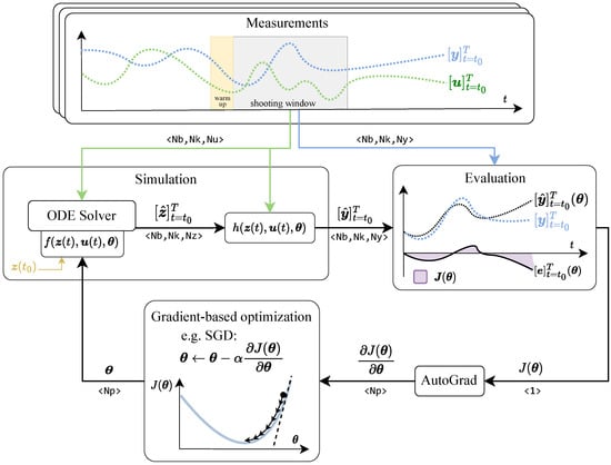
Figure 1.
Batched gradient-based parameter estimation framework of dynamical systems with automatic differentiation.
With this tool, we aim at learning an arbitrary dynamical system, described by continuous
or discrete
ordinary differential equations, where is the hidden dynamic state vector, represents the observable system output, which in this case is the friction torque , and is the input vector, which in this case is the angular velocity . We generalize different models by functions and , which are parameterized with free coefficients , which we intend to learn using the proposed framework. In fact, and can represent large neural networks, LSTMs, transformer models, or be a simple first-order differential equation, thus covering a wide range of white and black-box formulations.
Next, we consider that we dispose of measured system trajectories
each of them with samples. Note that we allow each trajectory to have different lengths and sample times. Since these data will be used to learn the model parameters, it is important to make them as informative as possible and to cover the entire dynamic operation range. By simulating the dynamical system, using the measured time and input sequences, we obtain the corresponding simulated outputs , which can be compared to the measured outputs and used as feedback to learn the model parameters . The dynamical system can be simulated either using Equation (3) with an ODE solver or using (4) directly. We describe the parameter estimation problem by minimizing the following prediction loss:
where is the loss function, which in this case is simply defined as the mean squared error over the trajectory and outputs. We then solve the problem above using gradient-based optimization techniques such as SGD, ADAM, etc. We implement a Runge–Kutta (RK) solver from scratch in JAX, so we can differentiate through the solver and thus the whole trajectory, analytically. Further, we extend all the functions required to calculate the loss, including the RK solver, so they support an additional batch dimension. With this, we can parallelize the computation in the GPU efficiently.
Moreover, the set represents a subset of all available data. We do this because differentiating analytically through long trajectories can be computationally expensive and lead to numerical instabilities when updating . Thus, we opt to resort to the so-called “shooting window” strategy, which was inspired by [64]. At each iteration, we randomly sample with replacement of the measured trajectories, and for each of them, sample a window position of size that fits the trajectory.
Another issue addressed in [64] is the problem of optimizing over trajectories with unobservable states. Even though this optimization procedure itself does not require measured state trajectories, the initial state is crucial. In many engineering problems, small changes in initial conditions produce large changes in trajectories. To overcome this problem, they augmented the parameter vector with the initial state of the shooting-window, which is referred to as “shooting variables” , and optimized them along the the model parameters . Nevertheless, in this work, we consider only friction models, which are known to be asymptotically stable systems, whose initial state contribution of the system vanish as time goes to infinity. The unobserved initial state is estimated in a “warm-up” phase, which is not used for optimization, right before the shooting window, by simulating the system with with the measured inputs . The calculated hidden state at the end of the warm-up phase is then used for optimization in the calculation of the loss function.
5. Ball Joint Friction Models
This section presents a series of phenomenological models describing ball joint friction. The modeling approaches begin with the three-dimensional LuGre friction model, which is formulated based on Velenis et al. [21] and incorporates the extension to three dimensions as suggested by Pfitzer et al. [22], followed by a simplified one-dimensional LuGre variant. Subsequently, a non-dynamic characteristic curve model is introduced, and finally, a highly flexible, black-box model based on long short-term memory (LSTM) neural networks is described.
All models are formulated in a standardized structure compatible with the model learning framework introduced in Section 4, following the system dynamics representations given in Equations (3) and (4). An overview showing the integration of each model into the shared learning framework is provided in Figure 2a.
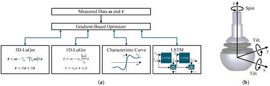
Figure 2.
Overview of the ball joint coordinate system and the benchmarked models. (a) Overview of model approaches. (b) Coordinate system and directions of the ball joint.
To ensure consistent model definition, the body-fixed coordinate system of the ball joints is defined as illustrated in Figure 2b. The coordinate origin is located at the center of the sphere with the z-axis aligned along the symmetry axis of the ball pin. The x- and y-axes are orthogonal to the z-axis, forming a right-handed coordinate system. Rotations around the x- and y-axes are referred to as tilt, while rotation around the z-axis is referred to as spin.
5.1. Three-Dimensional LuGre Model
As already noted in Section 1 and Section 3, ball joint friction exhibits velocity-dependent behavior. A widely used phenomenological approach for modeling such a friction behavior is the LuGre model. In its original form, it is defined as a one-dimensional model. However, as shown in Neumann [47] and Stietz [13], ball joint friction differs in spin and tilt directions, which necessitates a three-dimensional consideration of the phenomenon. Sorine and Szymanski [58] and later Velenis et al. [21] defined the LuGre model for two dimensions. In [65], a three-dimensional LuGre approach is presented for tire modeling, capturing the coupling of planar longitudinal and lateral friction as well as the self-aligning torque around the vertical axis. In contrast, in the preprint of a study by Pfitzer et al. [22], they mention the idea, based on the formulation in Velenis et al. [21], of extending the LuGre model to spherical contacts such as ball joints, where friction must be coupled across all three spatial directions. It is shown that the maximum dissipation principle, as described by Sorine [60], can be applied to compute the coupled friction torque within the fully three-dimensional framework used for macroscopic modeling.
The general form for the state change and the friction calculation of a multidimensional LuGre model defined in Velenis et al. [21] and reformulated in Pfitzer et al. [22] is given in Equations (7) and (8). The equations are expressed in a form that can be directly incorporated into the model learning formulation given in Equations (3) and (4). Equation (3) can be used to solve the differential equation continuously, and Equation (4) can be used when the equation is solved in discrete time steps. The quantities specified of the multidimensional LuGre model are defined in three dimensions to represent the spherical contact. Here, is the angular input velocity, is a diagonal matrix with the entries , and on the main diagonal that define the static friction torques, is the diagonal stiffness matrix, is the diagonal damping matrix of the state derivation, and is the state vector. The definition of the , K and D matrices are shown in Equation (9). It should be noted that the classical description of the LuGre model also contains a damping term which is directly dependent on the angular velocity . However, since this contradicts the Stribeck characteristic of friction, it is not considered in the following.
with
As shown in Figure 3, the friction torque moves within an ellipsoid defined by the entries of the matrix and the transient state factor . This factor scales the static friction ellipsoid in dynamic state changes and is therefore crucial for the dynamics of bristle models, such as the LuGre model. A detailed description of this factor can be found in Shao et al. [20]. It could be seen in Figure 3 that the bristle dynamics are represented in a global and macroscopic manner at the center of the ball joint by an ellipsoidal three-dimensional geometry, from which the friction properties are derived.
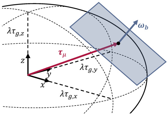
Figure 3.
Visualization of the three-dimensional friction ellipsoid.
The preprint of a study by Pfitzer et al. [22] includes additional model analyses, such as the distinction between stick and slip behavior, which can be easily incorporated into the model and, given suitable data, learned using the presented parameter estimation framework. However, this is not relevant for the intended application in online simulation for driving simulators aimed at evaluating driving comfort, as ball joints remain in continuous motion during operation. Furthermore, investigating static friction would require more elaborate tribological measurements, which cannot be performed with standardized component test rigs for ball joints, as described in Section 6.2.
Since is fundamental to the derivation of the LuGre description presented in Equation (7), it is already included in the equation and will not be further discussed. The friction ellipsoid ensures that the friction torque never exceeds the maximum of the torques in the rotation and tilt directions which is defined by Inequality (13) [21]. The direction of the friction force follows the Maximum Dissipation Principle and, as can be seen in Figure 3, is defined by the point where the LuGre bristle angular velocity is normal to the ellipsoid.
To provide the model with additional flexibility, the entries of the static of , K, and D are defined as functions. This is realized, as shown in Equations (10)–(12), through neural networks () which are individually trained based on the angular velocity and the internal state . The neural network algorithm is shown as a function in Algorithm 1. The input and output variables in lines 2 and 10 are scaled, which leads to a more favorable form of the error function for gradient descent optimization and thus to faster convergence [66]. In addition, line 3 ensures that the output variable is even symmetrical. The logarithm of the angular velocity is used, which results in higher resolution at low velocities. The neural network consists of two layers, using a combination of sigmoid functions to model nonlinear relationships. In a final step, the output variable is constrained by sigmoid functions using the limits and . It should be noted that the neural network can also depend on other parameters, which would result in the learning of multidimensional characteristic maps.
| Algorithm 1: Neural network used to learn the functions of the three-dimensional LuGre model. |
 |
Since the application of this model at driving simulators involves a hard real-time capability requirement, fixed time step solvers are applied. For that, it must be ensured that the LuGre differential equation is always solved in the shortest and most predictable time possible. This also implies that the model is discretized in time within the parameter estimation framework and solved using Equation (4). If the angular velocity is considered constant between time steps, then the ordinary differential Equation (7) can be written as a linear state space model
with the input , state space matrices and B = 1. This can be solved by
Assuming that the velocity remains constant in the interval , Equation (15) can be solved analytically as follows
Equation (16), in combination with Equation (8), can be used for solving the model in discrete time, as formulated in Equation (4).
Although the dynamic behavior of the LuGre model is preserved through linearization by embedding its differential equations into the A and B matrices, this process can introduce numerical challenges. As discussed in Section 6.3, the careful selection of parameter limits is therefore essential for each specific application. A comparison between the linearization presented as a solving method and using an ode45 solver is given in Appendix A. It is shown that linearization also leads to valid results in the case of highly dynamic excitations.
5.2. One-Dimensional LuGre Model
The first reference model is a classical, one-dimensional LuGre model by Canudas De Wit et al. [53], which, as described in Equation (17), is applied to each of the three spatial directions independently. As a result, the individual moments of friction in the spatial directions are independent of each other, and the resulting multidimensional friction force does not satisfy inequality (13), which leads to an overestimation of the friction force. The stiffnesses , the damping parameters , and the static friction torques are defined one-dimensionally, and it holds that . In addition, all these parameters are learned analogously to Equations (10)–(12) using the same neural network as in Algorithm 1 dependent on the velocity . The LuGre force is calculated according to Equation (18), where the stiffness matrix K and the damping matrix D, as shown in Equation (19), are defined analogously to Equation (9). Equations (17) and (18) are also formulated to allow direct integration into the model representations of Equations (3) and (4). The differential equations of the respective one-dimensional LuGre models are solved analogously to Equation (16), where it holds that and .
with
5.3. Characteristic Curves
The second reference model approach is a simple one-dimensional static characteristic curve, describing the friction torque as a function of the angular velocity. For the sake of simplicity, we decouple the 3 degrees of freedom and learn one characteristic curve per dimension.
To learn the characteristic curves with high flexibility, we use two fully connected neural networks with a minor extension to ensure the learned friction torque is symmetric around the origin of the velocity axis, which is a common assumption in static friction models. The model equations as well as the more detailed description of the neural network structure is provided in Equation (23) and Algorithm 2. This formulation can be applied directly as in Equation (4) for time-discrete systems.
| Algorithm 2: Neural network used to learn the functions of the characteristic curve. |
 |
5.4. LSTM Model
Introduced by [67], the long short-term memory (LSTM) networks are one of the most famous types of recurrent networks, which are designed to address the limitations of traditional RNNs, particularly in handling long-term dependencies. LSTMs are capable of learning and remembering information over long sequences, making them suitable for a variety of tasks including time-series prediction, natural language processing, and sequence modeling. In this paper, we utilize LSTM networks to learn a discrete differential equation of friction. The LSTM model’s ability to capture temporal dependencies allows it to effectively model the complex dynamics of friction. Although a multidimensional output formulation would be possible, we modeled one LSTM per output dimension compatible with the structure for time-discrete systems of Equation (4) as follows
where and are the LSTM hidden state and output at step k, respectively. We set their dimensions to 15. Finally, we concatenate the LSTM state vector to the input and add a single layer neural network to squeeze the dimensional output into a scalar torque value. The summary of these model operations are shown in Algorithm 3.
| Algorithm 3: Neural network used to calculate the torque from the LSTM states. |
 |
5.5. Model Summary
For a clear summary of the models, the properties of the four model approaches presented are shown in Table 1. The applicable characteristics are marked with an x. Since ball joint friction exhibits the characteristics of the Stribeck curve, velocity dependence is a fundamental property that has been taken into account in all model approaches. However, the three-dimensional LuGre model is the only model approach in which the degrees of freedom are coupled with each other. In terms of dynamic behavior, the characteristic curves model differs from the other models in that it has no dynamics. In the LuGre models, the dynamics are provided by the bristle properties. The LSTM model takes the dynamics directly from the measurement data due to its flexible black-box properties. This black-box property also distinguishes the LSTM model from the other model approaches. Thus, the model behavior of the LuGre models and the characteristic curve model is predetermined by the defined static friction characteristics and is therefore predictable as a white-box approach. In the LSTM approach, there are no openly visible model structures, which means that the model behavior cannot be predicted. Furthermore, the LSTM model differs from the other models in terms of continuity. The step size in the LSTM model is determined by the learning step size. If different step sizes are selected in the model, the LSTM model delivers implausible results. The basic model behavior of the other models, on the other hand, is independent of the selected step size.

Table 1.
Parameters of rheological models.
6. Operating Range Determination and Data Collection
Since we use a data-driven parameter estimation approach for our models, measurements of component behavior are required. To ensure that these measurements are within an application-relevant range of values, operating range measurements are needed. These operating range measurements are carried out as described below and serve as the basis for setting up a test program for component measurements in order to cover a range that is as accurate as possible. The component measurements will also be described and discussed.
6.1. Operating Range of Ball Joints
In order to determine the kinematic working ranges of ball joints, which serve as the basis for measurements on the kinematic component test bench, a high-comfort vehicle was equipped with measurement technology to record axle movement data on various tracks. The type of sensors and their positions are shown in Figure 4a, and the specifications are given in Appendix B. The aim of this analysis is to record the multidimensional movements of the axle using acceleration and laser measurements in order to then determine the angles and angular velocities occurring in ball joints. The ball joint of the lower control arm was selected as the ball joint to be investigated, as it plays an important role in several axle concepts [15]. The hybrid approach consisting of measurement and simulation used to determine the kinematic quantities of the ball joint is shown in Appendix D.
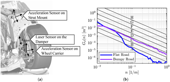
Figure 4.
Setup for operating range measurements. (a) Position and orientation of the acceleration sensors. (b) Unevenness density over the path frequency n together with classification according to ISO 8606, where it holds A = “very good evenness”, B = “good evenness”, C = “medium evenness”, and classes D–H = “cobblestone” to “off-road” tracks.
We collect data in four different road conditions. These include (I) a flat road, (II) a bumpy road, (III) a track with periodic impacts, and (IV) a track with sinusoidal wave excitations. The driving velocities and characteristics of the tracks are specified in Appendix E. The flat (I) and bumpy (II) roads can be classified into different track classes according to ISO 8608 [68], which is plotted in Figure 4b. Since ISO 8608 only applies to irregular excitations, a classification of the tracks with periodic excitations (III and IV) is not permissible. In the figure, the unevenness density spectrum is plotted over the track frequency n. In addition, the classifications of the respective areas according to ISO 8608 are plotted. The bumpy road (II) can be clearly assigned to classification C. Although the spectrum of the flat road (I) in the low-frequency range is in classification C, it can be assigned to classification A. The explanation for the classification of the flat road is shown in Appendix F. The track with periodic impacts (III) consists of concrete slabs arranged in such a way that an edge is created between the individual slabs. The length of the concrete slabs is between 4 m and 8 m, and the edge height is between 5 mm and 25 mm. The track with sinusoidal excitation (IV) also consists of concrete modules that have a sinusoidal shape with a synchronous wavelength of 12 m and an amplitude of 30 mm.
After the data have been collected by the four track measurements, they are post-processed using the techniques presented in Appendix D to determine the angular deviation and the velocity in the ball joint. The magnitudes of and are shown in Figure 5. It can be seen that the angular deflection hardly exceeds for the track excitations. For the sine waves, is exceeded at certain points. However, for the authentic track excitations, the displacement consistently remains below . For the angular velocity, it can be seen that angular velocities of over /s are also reached. However, the histograms show that the majority of the occurring angular velocities are below /s. Only the sine waves, which do not represent an authentic track signal, stand out there and have a comparatively constant velocity distribution in the range of /s. For the flat road, it can be observed that no velocity components above /s occur. For the concrete slab track with a periodic impact, it can be seen that the velocity distribution is a mixture of flat and bumpy road with the majority of the velocity distribution being below /s. This is due to the concrete slab surface corresponding to a flat road, and the edges represent isolated bumpy road excitations which can lead to angular velocities up to /s.
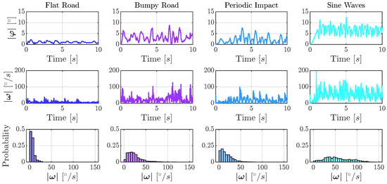
Figure 5.
Magnitudes of the operating ranges and probability distribution.
As insights for the system identification of the model, it could be gained that ball joints mainly operate in an operating range of . Furthermore, the velocity range of up to /s is particularly in focus. However, the model should also provide plausible values at angular velocities of over /s.
6.2. Measurement of Ball Joint Friction
Since it is technically hardly possible to reliably measure the friction torque of ball joints directly in the axle, component measurements are necessary to determine the friction behavior of ball joints. For this analysis, these component measurements are performed on a standardized component test bench from Brunel Car Synergies GmbH (44319 Dortmund, Germany). This allows for precise measurements of friction torque under various angular displacement amplitudes, angular velocities, excitement directions, and preload conditions. As schematically shown in Figure 6, the test bench setup consists of a torque measuring flange, a clamping device, and a force frame. The main component is the drive and measurement unit, which is located behind the torque measuring flange. The drive motor is electronically controlled, and the torque measuring flange is friction-optimized and hydraulically mounted. To simulate realistic load conditions, a static preload can be applied to the ball joint as indicated in the figure. The force can be applied in both axial and radial directions. The force is introduced via a force frame, which can be seen in the photo in Figure 6c below the control arm.
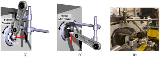
Figure 6.
Visualization of component test bench measurements of ball joints. (a) Visualization of spin measurements. (b) Visualization of tilt measurements. (c) Photo of a tilt measurement.
A flexible clamping situation consisting of rigid rods and joints allows the ball joint to be excited in different directions. The control arm is attached at a connection point to a damping mass, as there is no rubber bearing that would affect the measurement results due to its deformation. Figure 6a shows the measurement situation for spin excitation, and Figure 6b shows the measurement situation for tilt excitation. Additionally Figure 6c shows a picture of a tilt measurement. It should be noted that the control arm shown in the photo does not correspond to the control arm measured for this analysis. For spin measurements, the ball pin points in the direction of the rotation axis of the rotating flange and is directly connected to it. By rotating the flange, the ball joint is thus excited in the spin direction. For tilt excitation, the ball pin points orthogonally to the rotation axis of the rotating flange and is connected to it via a deflection geometry. This allows a tilt movement of the ball joint through the rotation of the flange.
For the first type of measurements, triangular signals of the angle were chosen as excitation. These have the advantage of having constant angular velocities, allowing a steady-state assignment between angular velocity and torque. Since the excitations in a real vehicle, as seen in Section 6.1, are usually dynamic, sinusoidal signals are also used as measurement excitations. The excitations are shown in Appendix G and are based on the findings from Section 6.1. The maximum amplitude of the triangular signals of the angular displacement is chosen as . Since the range in which the test bench is able to compensate for the torques of inertia of the masses is limited to angular velocities up to /s, this angular velocity was chosen as the maximum angular velocity for the measurements with triangular signal excitation. Figure 5 shows that most of the velocities occur in the range below /s, meaning that the measurements are able to cover the most common angular velocity range despite this limitation. Sinusoidal signals are applied up to , representing the natural frequency of the wheel, but with a small displacement amplitude of , resulting in velocities exceeding /s and thus the maximum permissible angular velocity range of the test bench.
Before the actual measurements, calibration measurements are conducted. During these calibration measurements, each excitation is carried out without a test object. This allows the friction and inertia of the test bench to be identified, which can then be compensated for in subsequent measurements.
Figure 7a shows the ball joint friction torque of a measurement with triangular excitation and a velocity of /s over the deflection angle . In the figure, a distinction is made between precycles and the actual measurement cycles, whereby it can be seen that the friction level changes significantly at the beginning of the measurement until a stationary range is reached. This illustrates that ball joint friction is heavily dependent on preconditioning [13] and that uniform preconditioning is of fundamental importance to ensure reproducible results. The preconditioning of ball joints for the component measurements is described in Appendix H and is based on specification AK-LH14 [33].
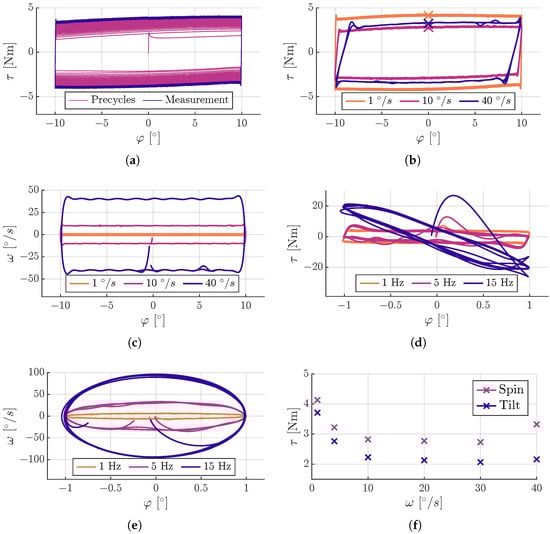
Figure 7.
Results from the ball friction measurements at the component test bench. (a) Change in friction torque during the precycles compared to the steady-state measurement area at /s in spin direction. (b) Measured friction torques at different angular velocities in spin direction with triangular excitation. (c) Measured angular velocities at different measurements in spin direction with triangular excitation. (d) Measured friction torques at different frequencies in spin direction with sinusoidal excitation. (e) Measured angular velocities at different frequencies in spin direction with sinusoidal excitation. (f) Velocity dependency of the friction torque in spin and tilt directions.
Figure 7b shows the friction torques measured at different velocities in the spin direction over the angular displacement . It can be seen that the hysteresis curve takes on a parallelogram shape with the sides sloping at higher angular velocity. Figure 7c shows the angular velocity over the angular displacement . As can be seen in the figure, the angular velocities have to build up over a certain time and thus over the displacement angle. This phenomenon becomes more apparent at higher angular velocities. In the measurements, it is not possible to implement the theoretically infinite acceleration at the reversal points of triangular angle signals. This leads to transient behavior, which also explains the different friction behavior in the areas of maximum deflection angle. Since reliable compensation of the test bench inertia in these transient ranges cannot be guaranteed, the test bench cannot be used to make reliable statements about the friction torque curve in the direction change ranges. This means that no reliable statements can be made about the stiffness of the friction phenomena.
Another limitation of the test bench measurement is shown in Figure 7d. The figure shows the friction torques of the sinusoidal measurements in the spin direction at different excitation frequencies. It can be seen that the curve at an excitation frequency of is still similar to the curves resulting from the triangular excitations in Figure 7c. However, the curves at higher excitation frequencies differ more significantly, as they have an additional slope. This slope increases with higher excitation frequencies, which leads to significantly increased friction torques. At an excitation frequency of , friction torque values of over occur. One reason for these implausibly high friction torques is provided by Figure 7e, which shows the angular velocities over the displacement angle . It can be seen that the angular velocity at an excitation of is significantly higher than the permissible excitation velocity of the test bench of /s. One consequence of this exceedance is that the inertial compensation of the test bench is no longer guaranteed, which leads to implausibly high measured friction torques. For this reason, only measurements up to and including , which do not exceed the permissible angular velocity of /s, are taken into account in the following.
In order to characterize the velocity dependence of the friction of the measured ball joint, the friction value is derived at the zero crossing of the deflection angles in the triangular measurements. This is determined as the mean value of the absolute values at the zero crossing and is shown as an example in Figure 7b. The values of the friction torque derived in this way are plotted in Figure 7f for the spin and tilt directions over the specified angular velocity. A classic Stribeck characteristic can thus be seen in the figure. It can also be seen that the friction torque in the tilt direction is lower than that in the spin direction. This could be explained by the fact that in the spin direction, contact is made across the entire equatorial diameter of the ball. In the tilt direction, this is not the case due to the opening for the ball pin at the top and the grease pockets at the bottom, which reduce the effective friction contact area. In addition, preload effects can influence the directional dependence of friction [13].
Data from measurements on the component test bench based on operating range measurements were collected. It was demonstrated that ball joints exhibit direction- and velocity-dependent behavior. In addition, undefined, transient characteristics of the test bench during direction changes and implausible torque curves at high velocities were identified and discussed. The plausible measurement data can now be used for parameter identification of the model approaches.
6.3. Data Selection and Parameter Estimation
The measurement data from the component tests described in Section 6.2 are used to identify the parameters of the models introduced in Section 5. As summarized in Table 2, the data are divided into training and test sets.
Table 2.
Training and test data for parameter identification.
For the LuGre-based and characteristic curve models, only static, velocity-dependent friction characteristics are trained. Since these require quasi-static conditions, only measurements with triangular excitation are used for training. As shown in Figure 7f, the velocities , , and represent characteristic points on the resulting Stribeck curve. Corresponding triangular measurements in both spin and tilt directions are used, noting that for tilt, identical data are applied to both directions due to unidirectional measurement.
Test data include triangular excitations at for extrapolation and for interpolation as well as sinusoidal excitations at various velocities within the test bench’s specification. Unlike triangular inputs, sinusoidal excitations generate continuously varying dynamic friction, making them suitable for evaluating model properties under dynamic excitation.
Training parameters as velocity-dependent neural networks leads to a large solution space, which may include regions that are physically implausible or unsuitable for real-time simulation. To ensure numerical stability and physical validity, parameter ranges were constrained as listed in Table 3 with all parameters restricted to positive values.
Table 3.
Hyperparameters for the LuGre models.
Given that measured friction torques during triangular excitations remained well below , this value was selected as the upper limit for the static friction characteristic . The model stiffness was limited to 10,000 Nm/rad to avoid excessive stiffness in real-time applications. For the damping parameter , an upper bound of was chosen, as higher values may result in non-physical torques [22].
It should be noted that the suitable bounds for and depend strongly on the overall system and may vary significantly. In this work, relatively high limits were intentionally selected to demonstrate the flexibility of the parameter learning approach, although such settings may already cause numerical problems in complex systems. A general proof of model stability in all vehicle environments is not feasible, as system-wide behavior cannot be directly inferred from subsystem properties. Therefore, the ranges of parameters should be carefully evaluated a priori for each specific application.
The described limits were chosen to be the same for both LuGre approaches. In addition, the limitation of the static friction characteristic was also applied to the characteristic curves model.
7. Results
In the following, we will discuss the fitting results and the properties of the models. The performance and suitability of the models are discussed in Section 7.6. In Appendix I, it is also shown how the cost functions of the presented parameter estimation framework for the compared models evolve over the iteration steps.
It should be noted that the model was trained solely as a function of angular velocity and direction. This is because no additional influences could be identified using the measurement procedures described in Section 6.2. Appendix J presents a series of measurements on the REMP with varying static preload in which no clear effect could be detected. The inclusion of this input variable in the model therefore does not appear to be reasonable. Other input variables, such as temperature, could theoretically also be taken into account, but these were not examined in this study. To incorporate these dependencies, as shown in the preprint of a study by Pfitzer et al. [22], the entries in the static friction matrix can also be learned as functions of several parameters, which can be collected in a general input vector . Due to the flexible structure of the parameter estimation framework given in Equations (3) and (4), learning dependencies on multiple parameters would be straightforward.
In the case of ball joint friction, it seems most reasonable to incorporate dependencies on other parameters, such as load, into the matrix. Ball joints have a frictional torque even without external load due to the preload given during the manufacturing process [13], making it a nonlinear dependency. Thus, a linear dependency of friction on the load according to the Coulomb definition of friction does not seem to be effective.
7.1. Fitting Results for Three-Dimensional LuGre Model
The results of the gradient-based optimization from Section 4 for the training data are shown in Figure 8, where simulated and measured torque profiles are compared over angular displacement and time t.
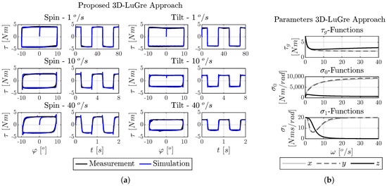
Figure 8.
Training results for the applied three-dimensional LuGre approach. (a) Fitting of the applied three-dimensional LuGre approach on the training data. (b) Parameters of the applied three-dimensional LuGre approach.
Figure 8b presents the learned model parameters as characteristic curves. As also observed in Figure 7f, the static friction torque is higher in the spin direction around the z-axis than in the tilt directions around the x- and y-axes. Due to identical training data, the tilt-direction parameters show consistent profiles. The parameters and also differ between spin and tilt directions and remain within the limits defined in Section 6.3.
Figure 8a further confirms that the model captures both the velocity and direction dependence of the friction. The slight torque increase at motion reversals is explained by higher static friction at low velocities and is further amplified by increased model stiffness.
In conventional LuGre models, the stiffness and damping parameters and are typically defined as constant values, which are set a priori. These parameters influence the shape of the hysteresis curves and can therefore also be learned from data. The velocity-dependent curves shown in Figure 8b cannot always be directly inferred from the measurements. Instead, they represent a local minimum that yields the best possible fit to the torque curve. As discussed in Section 6.3, parameter limits should be evaluated according to the specific application, taking into account factors such as the chosen model configuration, the general stiffness of the system, and the solver settings, to ensure numerical stability.
The result of the optimization is also influenced by the information contained in the training data. For example, dynamic excitation, which leads to state changes, is not present at high angular velocities in the triangular signals, which have constant angular velocities. Therefore, only limited information is available in this area for learning , which refers to the state change.
This study demonstrates the flexibility of gradient-based parameter learning within the framework introduced in Section 4. It reflects an application-specific trade-off between physical interpretability and fitting accuracy. For comparison, Appendix K presents a model with fixed values and , which are intentionally low to ensure a high potential of numerical stability. While this model yields reasonable accuracy (NRMSE: 0.2012), the model with variable parameters achieves a significantly better fit (NRMSE: 0.1288), highlighting the benefits of data-driven, velocity-dependent parameterization. To demonstrate that the presented parameter estimation framework leads to valid and reproducible model parameters, an analysis is presented in Appendix L. This analysis investigates, using synthetic training data from a simulation, whether the estimated parameters assume the same values as the parameters used to generate the synthetic data.
Figure 9 presents the fitting results for the test data. The model captures the direction- and velocity-dependent characteristics of the triangular excitation measurements well, although slight deviations in friction levels are observed. These differences can be attributed to the fact that the static friction curves were not explicitly trained at those velocity support points.
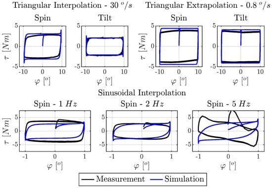
Figure 9.
Test results for the applied three-dimensional LuGre approach.
For sinusoidal excitations, the model produces plausible friction torque profiles at and with a slight underestimation at and a high-quality fit at .
At , the measured data show a general slope, likely caused by uncompensated inertia on the test bench, as discussed in Section 6.2. Since such effects are absent from the training data and the model does not include deflection-dependent stiffness, this behavior is not captured nor is it desirable. Despite this, the model still yields plausible torque predictions even under more dynamic conditions.
In summary, the three-dimensional LuGre model effectively reproduces the directional and velocity-dependent friction behavior of the ball joint across a range of operating conditions.
7.2. Fitting Results for the One-Dimensional LuGre Model
Figure 10 shows the results of the system identification of the one-dimensional LuGre model applied in independent spatial directions for the training data. The parameters are shown in Figure 10b, and it can be seen that the parameter characteristics are identical to those shown in Figure 8b for the three-dimensional LuGre approach. The fitting of the training and test data shown in Figure 10a and Figure 11 shows that the model behavior of the one-dimensional and three-dimensional LuGre models is identical. The similarity of the model behavior shown can be attributed to the fact that the excitation signals are one-dimensional signals, and the model differences are therefore not apparent.
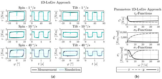
Figure 10.
Training results for the one-dimensional LuGre approach. (a) Fitting of the one-dimensional LuGre approach on the training data. (b) Parameters of the one-dimensional LuGre approach.
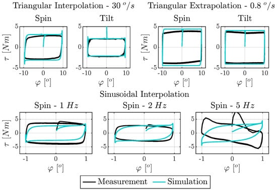
Figure 11.
Test results for the one-dimensional LuGre approach.
The one-dimensional modeling approach is therefore also capable of representing the velocity- and direction-dependent properties of ball joint friction. It is evident that the parameter estimation of the LuGre models independently leads to identical results.
7.3. Fitting Results for the Characteristic Curves Model
The results of the data fit and parameter estimation using the characteristic curve model are shown in Figure 12. Unlike the dynamic LuGre models, this approach captures only the static friction characteristics , as depicted in Figure 12b.
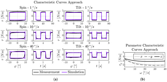
Figure 12.
Training results for the characteristic curves approach. (a) Fitting of the characteristic curves approach on the training data. (b) Parameters of the characteristic curves approach.
As it can be seen in Figure 8b, Figure 10b and Figure 12b, the fitted static friction torque differs between the LuGre-based models and the characteristic curve model. While the dynamic LuGre models yield values around , the static model converges to approximately . This discrepancy arises from the training data, as the measured torques do not start from zero and peak around –. The static model directly reflects these values, while the LuGre models compensate for unmeasured torque build-up near velocity zero crossings by increasing . This phenomenon could be prevented by using a lower upper limit for .
Due to the absence of dynamics, the friction torque depends directly on angular velocity. This leads to pronounced peaks at velocity reversal points, where low velocities result in high friction values. The lack of dynamic behavior of the model results in virtually infinite stiffness, amplifying this effect compared to the LuGre-based models.
The test data results in Figure 13 show that the characteristic curve model produces plausible friction torques across both interpolated and extrapolated velocity ranges. Overall, the modeled friction levels align well with the measurements. However, the absence of dynamic behavior becomes apparent in the sinusoidal excitations, where the model exhibits sharp transitions at velocity reversals, unlike the smoother measured profiles.
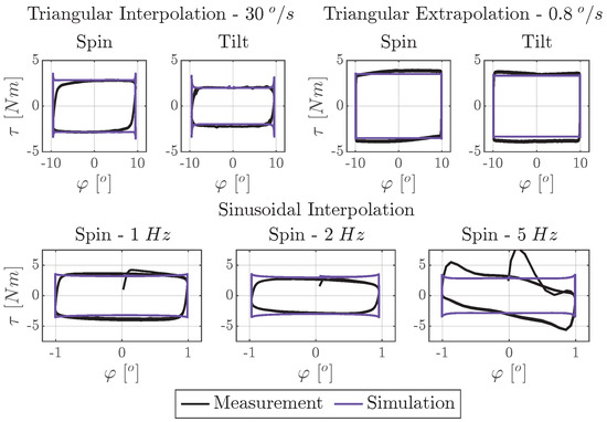
Figure 13.
Test results for the characteristic curves approach.
Nevertheless, the model effectively captures the velocity-dependent friction characteristics and allows differentiation between spin and tilt directions.
7.4. Fitting Results for the LSTM Model
Figure 14 shows the results of fitting the LSTM model approach to the training data. Since the LSTM model is a pure black-box model, no model parameters are shown in this case. It can be seen that the LSTM model replicates the measurement almost perfectly due to its high flexibility. The stiffness during direction changes and the static friction torques for both directions of movement and for all angular velocities are almost identical to the measurement. However, in the slow measurements of /s in the spin direction, a slight oscillation can be seen shortly after the direction changes.
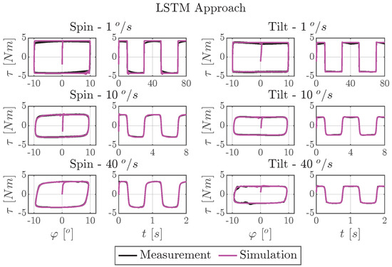
Figure 14.
Training results for the LSTM approach.
The tendency to oscillate is also present in the test data in the extrapolated case of /s in Figure 15. In this case, implausible oscillations occur in both the spin and tilt directions. In addition, at /s in the tilt direction, there is an overshoot of the friction torque, which does not occur in the model behavior of the training data in Figure 14. In the results with sinusoidal excitations, irregularities occur at the excitation frequency of , which are expressed by overshoots and a wavy pattern. The test data thus show that the LSTM approach can lead to irregularities and unpredictable properties.
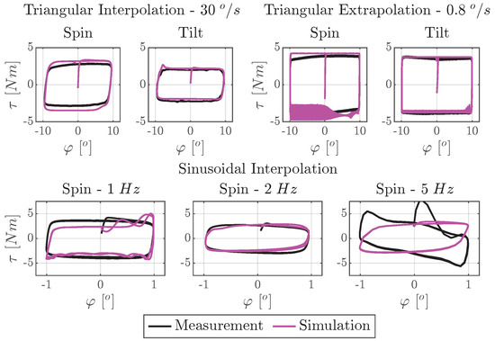
Figure 15.
Test results for the LSTM approach.
7.5. Synthetic Extrapolation of Model Approaches
As shown in Section 6.1, the operating ranges exceed the possible measurement ranges of the component measurements. It is therefore important that the models can deliver plausible values in the extrapolated range. To investigate this, two extrapolation cases and a multidimensional excitation are simulated and discussed in the following.
7.5.1. Extrapolation for High Angular Velocities
As shown in Figure 5, operational angular velocities can exceed , while the maximum angular velocity captured during measurement is limited to . To evaluate the model behavior outside this range, a synthetic triangular excitation with in the spin direction along the z-axis was applied, as shown by the dashed line in Figure 16.
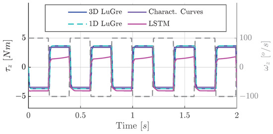
Figure 16.
Model behavior in an extrapolation range with a triangular excitation with an amplitude of at an angular velocity of /s in the z-direction.
The LuGre-based models in both one- and three-dimensional formulations show consistent and plausible extrapolated behavior, indicating that the learned static friction curves generalize well. The characteristic curve model produces a similar response. Due to the abrupt yet idealized sign changes in angular velocity, no overshoots occur in this case. Due to the transitionless but idealized sign change of the angular velocity, no overshoots occur in this case. In contrast, the LSTM model exhibits asymmetric and implausible behavior with significantly reduced friction values at negative velocities.
7.5.2. Extrapolation for Fast and Small Excitations
In complex multibody systems, coupling effects and time discretization can cause numerical phenomena such as rounding errors [69], which can lead to vibrations with low amplitude and high frequency even when the system is nominally at rest. To investigate model behavior under such conditions, a synthetic sinusoidal excitation with an angular displacement amplitude of and a frequency of was applied, corresponding to an angular velocity amplitude of approximately , as shown as a dashed line in Figure 17.
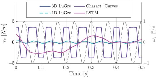
Figure 17.
Model behavior in an extrapolation range with a sinusoidal excitation with an amplitude of and a frequency of in the z-direction.
The LuGre models respond with minimal and consistent torque variations, demonstrating their dynamic behavior under small, fast excitations. In contrast, the characteristic curve model, lacking dynamic behavior, produces high friction torques even under minimal excitation.
The LSTM model again exhibits irregular and non-physical behavior. Its torque output remains negative for extended periods despite changes in the angular velocity direction, which may result in artificial energy generation.
The LuGre models also show a brief alignment between the direction of angular velocity and friction torque after reversals, which is a physically plausible outcome of their bristle-based formulation, where stored deformation energy is released during direction changes.
7.5.3. Model Behavior at Mixed Excitations
Due to limitations of the component test bench, only one-dimensional excitations could be used for parameter identification and model evaluation. However, ball joints are subject to multidimensional excitations that involve both spin and tilt. To evaluate the performance of the model under such conditions, phase-shifted sinusoidal angular velocity inputs were applied in the x, y, and z directions, each with an amplitude of and a frequency of , as shown in Figure 18a. The resulting torque magnitudes for the LuGre-based models are presented in Figure 18b.
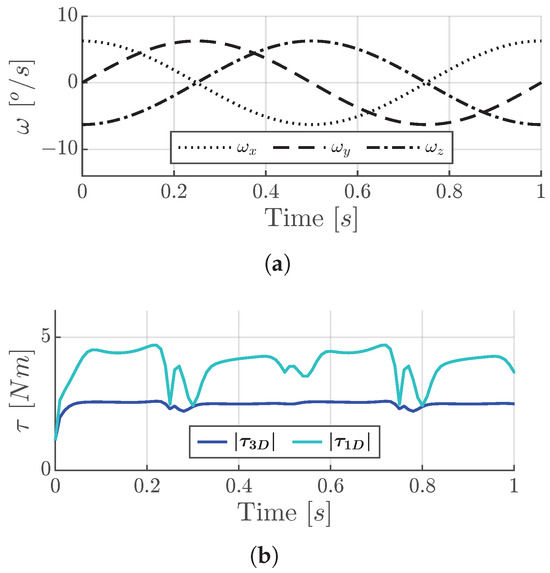
Figure 18.
Model behavior at mixed excitation with phase-shifted sinusoidal excitations with an amplitude of and a frequency of in the x-, y- and z-directions. (a) Input velocities. (b) Magnitude of torques.
While the one-dimensional LuGre model exhibited the same behavior as the three-dimensional LuGre model under isolated excitation, significant differences can be observed with multidimensional input. The torque magnitude is almost twice as large as in the three-dimensional LuGre model, which includes an ellipsoidal restriction on the combined torque, as shown in Figure 3. As noted by Kato [19], modeling friction in uncoupled degrees of freedom leads to an overestimation of the torque and violates the physical constraint specified in inequality (13).
In addition, the three-dimensional LuGre model exhibits smoother and more even torque curves, while the one-dimensional version produces abrupt changes at every velocity reversal.
7.6. Discussion of Results
Table 4 provides the NRMSE values for all model approaches. The LSTM model achieves the best results with an NRMSE of on the training data and on the test data. These values are significantly lower than those of the LuGre-based models, which perform similarly with training NRMSEs of for the three-dimensional LuGre and for the one-dimensional LuGre, and test NRMSEs of and , respectively. The characteristic curve model shows the highest NRMSE, with on training and on test data, indicating its limited ability to represent the system dynamics.
Table 4.
NRMSE of model approaches.
While the LSTM approach is characterized by high adaptation accuracy, its performance in extrapolated scenarios shows significant shortcomings. As shown in Section 7.5, the model exhibits irregular and non-physical behavior under high-frequency and low-amplitude excitations. Although the model exhibits the best data fit, these issues compromise its reliability and make it unsuitable for online simulations, especially in safety-critical applications such as driving simulators.
Although the characteristic curve model is simple, it lacks any dynamic behavior. As seen in Section 7.5.2, this leads to exaggerated torque responses under rapidly changing conditions and can cause numerical instability in simulations with fixed time steps.
Both LuGre-based models offer moderate accuracy with nearly identical NRMSE values. However, as seen in Section 7.5.3, only the three-dimensional LuGre model is capable of capturing the coupled multidimensional behavior required for ball joint friction. In contrast, the one-dimensional LuGre model treats each degree of freedom independently, which leads to an overestimation of the torque in combined spinning and tilting movements. The three-dimensional LuGre model avoids this by imposing an ellipsoidal constraint, thus producing smoother and more physically plausible responses.
Overall, while the LSTM model provides the best numerical fit to the training and test data, the three-dimensional LuGre model achieves the best balance between accuracy, physical plausibility, and robustness—making it the most suitable choice for real-time applications.
8. Conclusions
This work presented a universal, gradient-based framework for parameter estimation for the identification and training of phenomenological ball joint friction models with a special focus on real-time online simulation in the context of driving simulation. The framework enables the efficient learning of differentiable dynamic models from experimental data and was applied to train and evaluate four different modeling approaches:
- The three-dimensional spherical LuGre model based on the definition from Velenis et al. [21] and the reformulation from Pfitzer et al. [22];
- A one-dimensional LuGre model;
- A static characteristic curve model; and
- A black-box long short-term memory (LSTM) model.
To support realistic model development, measurements of the operating range of ball joints were carried out under real driving conditions. For this purpose, an optimized method for signal integration for acceleration data was developed. The results showed that ball joints typically operate in an angular range of less than and at angular velocities below . However, the measurements also showed that angular velocity peaks of over can occur. Based on these results, measurements were carried out on a standardized component test bench. These tests revealed clear differences between spinning and tilting movements and confirmed a velocity-dependent behavior of the friction torque.
All models were trained using the same gradient-based optimization framework and evaluated using a shared test dataset as well as in synthetic extrapolation scenarios. The main findings are summarized below:
- Parameter Estimation Framework: The proposed method enables the efficient and reproducible identification of parameters in differentiable dynamic models. It supports the integration of both physically motivated and black-box model structures within a single optimization framework.
- Model Fitting Accuracy: The LSTM model achieved the highest numerical accuracy, showing an NRMSE of 0.0482 on the training dataset and 0.1887 on the test dataset. Both LuGre-based models followed closely, with NRMSE values near 0.13 for training data and 0.26 for test data. The static characteristic curve model showed the lowest performance with errors of 0.2711 on the training set and 0.3021 on the test set.
- Extrapolation Behavior and Robustness: While the LSTM model produced highly accurate results within the training domain, its behavior in extrapolated conditions was irregular, asymmetric, and physically implausible. This disqualifies it from use in real-time or safety-critical applications such as driving simulators.
- Numerical Stability of the Static Model: The characteristic curve model does not capture dynamic effects. As a result, it generates excessively large torque values under fast or small excitations, which can cause numerical instability in fixed-step simulations.
- Best Overall Performance—Three-Dimensional LuGre Model: Among the evaluated approaches, the three-dimensional LuGre model demonstrated the best balance between fitting accuracy, physical realism, and numerical robustness. Its ellipsoidal coupling of rotational degrees of freedom enables smooth and consistent torque behavior under multidimensional excitations.
In summary, the combination of a general gradient-based learning framework with standardized component-level test bench data enables the reliable identification of friction models for ball joints. The three-dimensional LuGre model was identified as the most promising candidate for use in vehicle simulation environments, offering both physical accuracy and numerical stability across the full range of relevant operating conditions.
Future work may involve extending the parameter estimation framework to other use cases. The three-dimensional LuGre model can also be integrated into complete vehicle dynamics models to investigate the influence of ball joint friction on driving behavior, handling performance, and ride comfort.
Author Contributions
Conceptualization, K.P. and L.R.; methodology, K.P. and L.R.; software, K.P. and L.R.; validation, K.P. and L.R.; formal analysis, K.P.; investigation, K.P.; resources, K.P.; data curation, K.P.; writing—original draft preparation, K.P.; writing—review and editing, S.K., B.C. and G.P.; visualization, K.P.; supervision, S.K. and G.P.; project administration, K.P. All authors have read and agreed to the published version of the manuscript.
Funding
This research received no external funding.
Data Availability Statement
The data an model can be found at github/balljoint-friction-fitting (https://github.com/lucasrm25/balljoint-friction-fitting, accessed on 19 September 2025).
Conflicts of Interest
Authors Kai Pfitzer, Lucas Rath and Sebastian Kolmeder were employed by the company BMW Group. The remaining authors declare that the research was conducted in the absence of any commercial or financial relationships that could be construed as a potential conflict of interest.
Appendix A. Performance Linearization
Figure A1 presents the comparison of a LuGre model solved using different methods: the linearization described in Section 5.1 and an ode45 solver under highly dynamic excitation. It is evident that deviations from the ground truth simulated with a smaller step size are minimal in both cases. The NRMSE of the ode45 solver compared to the ground truth is 0.0017, and the proposed linearization is 0.0170. This shows that while the ode45 solver with a variable step size of max s is more accurate, the characteristics of the LuGre model are preserved with the proposed linearization, which enables a real-time solution using a fixed step size. The absolute error represented by the two solution methods with s remains below Nm. Thus, it has been demonstrated that solving through linearization is also permissible under highly dynamic excitations and leads to plausible results.

Figure A1.
Comparison between the LuGre model solved with an ode45 solver and the linearization proposed in Section 5.1 using a sinus sweep as the input signal for angular velocity . The sweep has an amplitude of /s and increases linearly from 1 to 50 Hz over a duration of 5 s. The LuGre model was parameterized with Nm/rad, Nms/rad, and a analogous to the measurement results from Section 6.2. As ground truth, a simulation was performed with an ode45 solver and a maximum step size of s. To benchmark the linearization, a simulation was performed with the ode45 solver using the same maximum step size of s. The resulting friction torques are depicted along with a zoom into the final, highly dynamic oscillations. The zoom also shows the difference between the results obtained with the ode45 solver and the linearization with the same maximum step size of s.

Appendix B. Sensor Specification
As shown in Figure 4a, acceleration sensors are installed on the strut mount and the wheel carrier of the vehicle. The sensors are triaxial Micro-Electro-Mechanical System (MEMS) sensors that are also able to record low-frequency acceleration signals. The sensor specifications are given in Table A1. Since lower-frequency signals are to be expected at the main body of the vehicle, sensors with a lower maximum value range were installed on the strut mount.
Table A1.
Specification of the MEMS sensors.
Table A1.
Specification of the MEMS sensors.
| Property | Strut Mount | Wheel Carrier |
|---|---|---|
| Type | Dytran Instruments 7556A1 | PCB 3713B1150G |
| Input Range | ±29.43 m/s2 | ±490.5 m/s2 |
| Frequency Range (PI) | 0–800 Hz | 0–1000 Hz |
Appendix C. NRMSE
The normalized root mean squared error (NRMSE) used in this work is given by
Appendix D. Determination of Operation Ranges
The procedure of the hybrid approach to determine the angular displacement and angular velocity is illustrated in Figure A2 and is explained in the following. As it can be seen from the figure, the suspension movements are recorded in the form of acceleration signals. The coordinate system of the strut mount is oriented differently than the coordinate system of the wheel carrier. To transform the accelerations at the strut mount into the coordinate system of the wheel carrier, the acceleration signal of the strut mount is multiplied by the rotation matrix . After that, the acceleration signals from the strut mount and from the wheel carrier are then subtracted from each other to determine the relative acceleration of the wheel carrier to the vehicle body.

Figure A2.
Illustration of the process of determining the value range.
Figure A2.
Illustration of the process of determining the value range.

To obtain the relative displacement from the relative acceleration, a double integration is necessary. To avoid numerical errors and for better handling [70], this integration is performed in the frequency domain. Since low-frequency measurement errors have a strong influence during integration and the recorded acceleration of gravity leads to a drift of the signal, it is necessary to filter the signals with a high-pass filter [71].
The optimal cutoff frequency is determined iteratively. For this, an additional control signal to the acceleration signals is needed. Therefore, the displacement of the damper was recorded using a laser sensor. For the optimization of the cutoff frequency, the z-component of the integrated relative displacement is compared with the damper displacement. For the comparison between wheel carrier movement and damper displacement to be valid, the damper displacement must first be multiplied by a displacement dependent damper ratio . The NRMSE is chosen as the quality measure and is defined in Appendix C.
Figure A3a shows the influence of the high-pass filter cutoff frequency on the NRMSE between the integrated wheel carrier displacement in the z-direction and the damper displacement transformed in the z-direction. It can be seen that the NRMSE assumes high values for all signals at a cutoff frequency close to . This is due to the drift of the integrated acceleration signals caused by signal components such as gravitational acceleration and higher-weighted measurement errors in the low-frequency range. With increasing cutoff frequencies, the NRMSE decreases and a valley forms in which the minimum is found for all signals. It can also be seen that the NRMSE is worst for signals with small excitations from the flat road and best for signals with periodic excitations. One explanation for this could be that signals with large, sudden accelerations are easier to measure with the acceleration sensors [72]. As the cutoff frequency increases, the NRMSE values are becoming worse again. This can be observed particularly in the tracks with periodic impacts and sine waves as excitation, where the NRMSE jumps up. This is because above a certain frequency, the excitation frequencies of the concrete slabs and modules are filtered out and the displacement signal generated then only contains high-frequency side effects.

Figure A3.
Cutoff frequency and fitting result of the optimized integration method. (a) Influence of the cutoff frequency on the NRMSE. (b) Fitted displacement signals in comparison to the translated damper way in z-direction.
Figure A3.
Cutoff frequency and fitting result of the optimized integration method. (a) Influence of the cutoff frequency on the NRMSE. (b) Fitted displacement signals in comparison to the translated damper way in z-direction.

Figure A3b shows the determined displacement signals together with the translated damper displacements in the time domain. It can be seen that the integrated signal lacks some low-frequency signal components compared to the damper signal. This is particularly noticeable for the sine waves, where the longer-lasting displacements are not perfectly captured. Nevertheless, it can also be seen that the value ranges are captured by the filtered and integrated acceleration signals.
To consider the complete motion information of the wheel carrier, the acceleration values in the x- and y-directions and are also integrated. For this purpose, the cutoff frequency optimized previously via the z-component is also applied to the x- and y-components of the signal. After the individual integration of all acceleration signals, they can be combined again to form the three-dimensional movement of the wheel carrier . To obtain the needed angular displacement and angular velocity of the ball joint from the wheel carrier movements, the motion information is used as input for a kinematic model of the suspension. Since high-frequency noise in a discrete, numerical simulation would also lead to strongly noisy simulation signals, the signals are smoothed beforehand with a low-pass filter. Since the focus of the model is on body vibration comfort, signals above , which only have acoustic relevance [73], are filtered out.
Appendix E. Specification of Tracks
Table A2.
Specification of the tracks.
Table A2.
Specification of the tracks.
| Track | Velocity | Description |
|---|---|---|
| Flat Road (FR) | 60 km/h | ISO 8608 Classification A |
| Bumpy Road (BR) | 80 km/h | ISO 8608 Classification C |
| Periodic Impact (PI) | 20 km/h | Concrete slabs with edges |
| Sine Waves (SW) | 60 km/h | Concrete modules with sinus shape |
Appendix F. Classification of the Flat Road
At low frequencies up to a track frequency of n = 0.03 1/m, the bumpy and flat roads according to ISO 8608 are hardly distinguishable from each other. In addition, the flat road can only be assigned to classification A from n = 0.05 1/m. Based on the following consideration, the flat road can nevertheless be clearly assigned to classification A.
The vehicle velocity on the even road is = 60 km/h. Together with the path frequency n, the resulting vehicle excitation can be calculated using Equation (A2).
As the excitation frequency is significantly below the body’s natural frequency of approx. , it can be assumed that this low-frequency excitation has only a minor and negligible influence on the movement of the vehicle axle.
Appendix G. Measurement Program of the Component Test Bench
Table A3.
Measurement program for component measurements at the REMP.
Table A3.
Measurement program for component measurements at the REMP.
| Measurement in Spin and Tilt Direction | |||||
|---|---|---|---|---|---|
| Axial Preload of 5 kN | |||||
| Triangular Angle Signal | Sinusoidal Angle Signal | ||||
| Pos | Angle | Angular | Pos | Angle | Frequency |
| Velocity | |||||
| 1 | /s | 9 | |||
| 2 | /s | 10 | |||
| 3 | /s | 11 | |||
| 4 | /s | 12 | |||
| 5 | /s | 13 | |||
| 6 | /s | ||||
| 7 | /s | ||||
| 8 | /s | ||||
Appendix H. Preconditioning of Ball Joints
To ensure even distribution of the lubricating grease, the ball joints are preconditioned by manual tumbling movements before being clamped into the test bench. Subsequently, 20 pre-cycles are run on the test bench so that, as can be seen in Figure 7a, grease displacement effects and the resulting transient behavior of the friction torque have no influence on the measurements. After the five measurement cycles, a decay cycle is run so that a decay in the test bench velocity also has no influence on the measurements.

Figure A4.
Illustration of the test bench preconditioning of ball joints.
Figure A4.
Illustration of the test bench preconditioning of ball joints.

Appendix I. Parameter Estimation Performance over Iterations
Figure A5 illustrates the cost function, represented by the RMSE, for the respective learned models that need to be minimized. It can be observed that the cost function for the LuGre models quickly assumes low and constant values. This can be attributed to the fixed structure of the LuGre models with defined parameters, which positively impacts the learning process by restricting the degrees of freedom. In contrast, the characteristic curves model, which lacks a fixed structure, takes more iterations to achieve stable, low values compared to the LuGre models. Furthermore, it is evident that the value of the cost function achieved is the highest among the models compared. The LSTM model also requires more iterations to reach a constant minimal value, but it achieves the lowest value. Furthermore, it is noticeable that the LSTM model starts from the highest point on the path to the lowest value and exhibits some high fluctuations in the course of the cost function. This can be attributed to the high dynamic flexibility of the model, which may lead to iterations in local minima.

Figure A5.
Cost function values over iteration steps for all learned models.
Figure A5.
Cost function values over iteration steps for all learned models.

Appendix J. Influence of Load
In addition to the measurements presented in Section 6.2, the influence of a static preload was investigated using the REMP. For this purpose, the axial preload was varied from 0 to . The resulting measured friction torques, determined analogously to Figure 7b, are shown in Figure A6. In this representation, the static friction torque is plotted as a function of the static axial force . The results indicate only minor variations in the friction torque with no clear trend emerging from the measurements. A plausible explanation for this observation is a trade-off between two opposing mechanisms: (i) degraded contact properties caused by elastic deformation of the ball socket at higher loads and (ii) improved lubrication performance due to high loads.

Figure A6.
Measured influence of load on ball joint friction.
Figure A6.
Measured influence of load on ball joint friction.

Appendix K. Model Fitting with Constant σ0 and σ1

Figure A7.
Results for the applied three-dimensional LuGre approach with constant Nm/rad and Nms/rad.
Figure A7.
Results for the applied three-dimensional LuGre approach with constant Nm/rad and Nms/rad.

Appendix L. Reproduction of Predefined Parameters
To test whether the parameter estimation framework leads to reproducible and plausible parameters, synthetically generated data from a simulation are used as training data below. The objective is to investigate whether the framework is capable of reproducing the parameters used to generate the training data.
The data generation process, as well as the inputs and outputs of the framework, are depicted in Figure A8a. The generated time signals , , and are shown in Figure A8b. Unlike with measurements, it is also possible to learn the static friction curves using dynamic signals with synthetic data because the dynamic and static components are clearly distinguishable by the framework. In measurements, this distinction is not possible due to potential and unknown measurement errors, as mentioned in Section 6.3.
The values of the cost function, represented by RMSE values, are shown over the iteration steps in Figure A9. It becomes apparent that the dispersion of the values is higher compared to the trend shown in Figure A5, where real measurement data were used as training data. This can be attributed particularly to the lack of variance in the synthetic signals at small angular velocities. Since few events, like direction changes, occur at small angular velocities, the framework encounters challenges in accurately modeling this region owing to the lack of sufficient informational input. Thus, higher errors occur in iteration steps where windows from this area are considered more frequently. This phenomenon could be counteracted with larger window sizes or more data from the low-velocity range.

Figure A8.
Generation of synthetic training data. (a) Workflow illustrating how a synthetic torque signal is determined using a LuGre model with predefined parameters of Nm/rad, Nms/rad, and a analogous to the measurement results from Section 6.2. A synthetic angular velocity signal derived from an angular signal serves as the input. The synthetic angular velocity signal and the determined torque signal are subsequently used as training inputs for the parameter estimation framework introduced in Section 4. This framework learns the 3D-LuGre model described in Section 5.1 with excitation only in the z-direction. The parameter estimation framework then outputs the estimated parameters , , and as well as the resulting torque profile . (b) Representation of the time signals of the angular signal , the angular velocity signal , and the determined friction torque . The angular velocity signal is derived from a sinusoidal sweep signal of the angle with an amplitude of , increasing from to within s.


Figure A9.
Cost function values over iteration steps.
Figure A9.
Cost function values over iteration steps.

In Figure A10, the outputs of the parameter estimation framework are presented. The axis scaling of the parameters represents the respective limits within which they were learned. It is evident that the estimated parameters are each close to the predefined, true parameters. One reason for the slight deviations could be that linear interpolation was applied to in the simulation for generating the synthetic data. This linear connection of the individual points can only be partially represented by the applied sigmoid functions in the parameter estimation framework. This deviation of can lead to compensation by other parameters. Additionally, deviations are observed in and at low angular velocities. This can also be explained by the previously described, poor information situation in the low-velocity range of the training data. However, it is evident that there is a high similarity between the estimated parameters and the predefined, true parameters. This is also shown in the comparison of the synthetic moment , which was used as training data, and the learned . With an NRMSE of 0.0447, there is a high consistency between the training data and the learned data. In this way, it was demonstrated that the presented parameter estimation framework, despite its high flexibility, is capable of generating plausible and reproducible parameters as output.

Figure A10.
Comparison between the predefined, true parameters and the parameters estimated by the parameter estimation framework, as well as a comparison between the profile of the synthetic training input torque and the torque resulting from the estimated parameters. The limits of the learned parameters correspond to the scaling of the y-axis. The following limits were chosen: Nm, Nm/rad, Nms/rad.

References
- Schramm, D.; Hiller, M.; Bardini, R. Modellbildung und Simulation der Dynamik von Kraftfahrzeugen; Springer: Berlin/Heidelberg, Germany, 2018. [Google Scholar] [CrossRef]
- Huber, W. Industrie 4.0 in der Automobilproduktion; Springer Fachmedien Wiesbaden: Wiesbaden, Germany, 2016. [Google Scholar] [CrossRef]
- Nan, J.; Ge, Z.; Ye, X.; Burke, A.F.; Zhao, J. Model predictive control for autonomous vehicle path tracking through optimized kinematics. Results Eng. 2024, 24, 103123. [Google Scholar] [CrossRef]
- Martin, S.; Schütte, J.; Bäumler, C.; Sextro, W.; Tröster, T. Identification of joints for a load-adapted shape in a body in white using steady state vehicle simulations. Forces Mech. 2022, 6, 100065. [Google Scholar] [CrossRef]
- Winner, H.; Hakuli, S.; Lotz, F.; Singer, C. Handbook of Driver Assistance Systems; Springer International Publishing: Amsterdam, The Netherlands, 2016. [Google Scholar] [CrossRef]
- Pech, D.; Dessort, R.; Prokop, G. Experimental parameter identification of scalable white and grey box jounce bumper models for ride comfort simulation. Veh. Syst. Dyn. 2024, 63, 1625–1648. [Google Scholar] [CrossRef]
- Troulis, M.; Gnadler, R.; Unrau, H.J. Übertragungsverhalten von Radaufhängungen für Personenwagen im komfortrelevanten Frequenzbereich. ATZ-Automob. Z. 2004, 106, 336–348. [Google Scholar] [CrossRef]
- Xuwang, W.; Chen, X.; Xu, P.; Zhang, Y. The Effect of Friction on Ride Comfort Simulation and Suspension Optimization; SAE International: Warrendale, PA, USA, 2020. [Google Scholar] [CrossRef]
- Angrick, C.; Prokop, G.; Knauer, P.; Wagner, A. Improved prediction of ride comfort characteristics by considering suspension friction in the automotive development process. In 6th International Munich Chassis Symposium 2015: Chassis. Tech Plus; Springer Fachmedien Wiesbaden: Wiesbaden, Germany, 2015; pp. 377–403. [Google Scholar] [CrossRef]
- Matheus, A.D.C.; De Oliveira, W.R.; Villani, E. A Safety-Oriented Motion Cueing Algorithm for a Serial Robotic Flight Simulator Using a Predictive Neural Network Reference Governor. IEEE Trans. Intell. Transp. Syst. 2024, 25, 15718–15731. [Google Scholar] [CrossRef]
- Official Journal of the European Union: Directive 2006/42/EC Annex IV. 2006. Available online: https://eur-lex.europa.eu/eli/dir/2006/42/oj/eng (accessed on 19 September 2025).
- Miller, S.; Wendlandt, J. Real-Time Simulation of Physical Systems Using Simscape™. In Real-Time Simulation Technologies; Series Title: Computational Analysis, Synarticle, & Design Dynamic Systems; CRC Press: Boca Raton, FL, USA, 2012; Volume 13, pp. 581–598. [Google Scholar] [CrossRef]
- Stietz, T. Bewegungsverhalten von Kugelgelenken in Fahrzeugachsen im Akustisch Relevanten Frequenzbereich; Springer Fachmedien Wiesbaden: Wiesbaden, Germany, 2018. [Google Scholar] [CrossRef]
- Smyrek, C. Simulation der Stillstandszeitabhängigen Losbrechkraft im Mischreibungskontakt Mittels Eines Viskoelastischen Ansatzes. Ph.D. Thesis, Ruhr-Universität Bochum, Bochum, Germany, 2021. [Google Scholar] [CrossRef]
- Wozniak, M.; Siczek, K.; Ozuna, G.; Kubiak, P. A Study on Wear and Friction of Passenger Vehicles Control Arm Ball Joints. Energies 2021, 14, 3238. [Google Scholar] [CrossRef]
- Dahl, P.R. A Solid Friction Model; The Aerospace Corporation: El Segundo, CA, USA, 1968. [Google Scholar] [CrossRef]
- De Wit, C.C.; Olsson, H.; Astrom, K.; Lischinsky, P. Dynamic Friction Models and Control Design. In Proceedings of the 1993 American Control Conference, San Francisco, CA, USA, 2–4 June 1993; pp. 1920–1926. [Google Scholar] [CrossRef]
- Johanastrom, K.; Canudas-de Wit, C. Revisiting the LuGre friction model. IEEE Control Syst. 2008, 28, 101–114. [Google Scholar] [CrossRef]
- Kato, H. Friction model for planar two-dimensional motion. In Proceedings of the IECON 2015—41st Annual Conference of the IEEE Industrial Electronics Society, Yokohama, Japan, 9–12 November 2015; pp. 000220–000225. [Google Scholar] [CrossRef]
- Shao, R.; Wahle, M.; Zimmermann, M. A model for the dynamic friction behaviour of rubber-like materials. Tribol. Int. 2021, 164, 107220. [Google Scholar] [CrossRef]
- Velenis, E.; Tsiotras, P.; Canudas-de Wit, C. Extension of the lugre dynamic tire friction model to 2d motion. In Proceedings of the 10th IEEE Mediterranean Conference on Control and Automation-MED, Lisbon, Portugal, 9–12 July 2002. [Google Scholar]
- Pfitzer, K.; Rath, L.; Kolmeder, S.; Corves, B.; Prokop, G. A General Mechanical Formulation of Two-Dimensional Bristle Friction Models with a Focus on the Lugre Model and its Dynamics. SSRN 2025, preprint. [Google Scholar] [CrossRef]
- Ljung, L. System Identification. In Signal Analysis and Prediction; Procházka, A., Uhlíř, J., Rayner, P.W.J., Kingsbury, N.G., Eds.; Birkhäuser Boston: Boston, MA, USA, 1998; pp. 163–173. [Google Scholar] [CrossRef]
- Bradbury, J.; Frostig, R.; Hawkins, P.; Johnson, M.J.; Leary, C.; Maclaurin, D.; Necula, G.; Paszke, A.; VanderPlas, J.; Wanderman-Milne, S.; et al. JAX: Composable Transformations of Python+NumPy Programs. 2018. Available online: https://github.com/jax-ml/jax (accessed on 19 September 2025).
- Paszke, A.; Gross, S.; Massa, F.; Lerer, A.; Bradbury, J.; Chanan, G.; Killeen, T.; Lin, Z.; Gimelshein, N.; Antiga, L.; et al. PyTorch: An Imperative Style, High-Performance Deep Learning Library. arXiv 2019, arXiv:1912.01703. [Google Scholar]
- Trinh, M.; Pellenz, Y.; Gruendel, L.; Petrovic, O.; Becher, C. Modeling of Load-dependent Friction in Robot Joints Using Long Short-term Memory Networks. In Proceedings of the ISR Europe 2023: 56th International Symposium on Robotics, Stuttgart, Germany, 26–27 September 2023; pp. 46–53. [Google Scholar]
- Cortes, G.; Garcia-Suarez, J. Data-Driven Dynamic Friction Models based on Recurrent Neural Networks. arXiv 2025, arXiv:2402.14148. [Google Scholar] [CrossRef]
- Ozmen, A.; Hespanha, J.P.; Byl, K. Learning Transferable Friction Models and LuGre Identification via Physics Informed Neural Networks. arXiv 2025, arXiv:2504.12441. [Google Scholar] [CrossRef]
- Gupta, J.K.; Menda, K.; Manchester, Z.; Kochenderfer, M.J. A General Framework for Structured Learning of Mechanical Systems. arXiv 2019, arXiv:1902.08705. [Google Scholar] [CrossRef]
- Lutter, M.; Silberbauer, J.; Watson, J.; Peters, J. A Differentiable Newton Euler Algorithm for Multi-body Model Learning. arXiv 2020, arXiv:2010.09802. [Google Scholar] [CrossRef]
- Geist, A.R.; Trimpe, S. Structured learning of rigid-body dynamics: A survey and unified view from a robotics perspective. arXiv 2020, arXiv:2012.06250. [Google Scholar] [CrossRef]
- Lutter, M.; Peters, J. Combining Physics and Deep Learning to learn Continuous-Time Dynamics Models. arXiv 2023, arXiv:2110.01894. [Google Scholar] [CrossRef]
- Specification AK-LH14—Working committee of the following companies: Audi AG, Bayerische Motoren Werke AG, DaimlerChrysler AG, Porsche AG, Volkswagen AG. Unpublished work. 2004.
- Sage, R.M. The Mathematical Modelling of Ball-Joints with Friction; University of Leicester: Leicester, UK, 1987. [Google Scholar]
- Wu, J.; Li, W.; Xiong, Z. Identification of robot dynamic model and joint frictions using a baseplate force sensor. Sci. China Technol. Sci. 2021, 65, 30–40. [Google Scholar] [CrossRef]
- Trinh, M.; Schwiedernoch, R.; Gründel, L.; Storms, S.; Brecher, C. Friction Modeling for Structured Learning of Robot Dynamics. In Production at the Leading Edge of Technology; Springer: Cham, Switzerland, 2023; pp. 396–406. [Google Scholar] [CrossRef]
- Corrêa Do Lago, A.W.; Braz De Sousa, D.H.; Domingues, P.H.; Daneker, M.; Lu, L.; Hultmann Ayala, H.V. Physics-informed and black-box Identification of robotic actuator with a flexible joint. IFAC-PapersOnLine 2024, 58, 259–264. [Google Scholar] [CrossRef]
- Chen, S.; Cheng, G.; Pang, Y. Dynamic Analysis and Trajectory Tracking Control for a Parallel Manipulator with Joint Friction. Appl. Sci. 2022, 12, 6682. [Google Scholar] [CrossRef]
- Leguet, G.D.; Roche, J.F.; Hamdi, M.A.; Rachik, M. Investigation of ball joints under static and dynamic loads. In Proceedings of the 7th European Conference for Aeronautics and Space Sciences (EUCASS), Milan, Italy, 3–6 July 2017; p. 14. [Google Scholar] [CrossRef]
- Kang, J. The onset condition of friction noise in ball joint under concentric loading. Appl. Acoust. 2015, 89, 57–61. [Google Scholar] [CrossRef]
- Kang, J. Theoretical Model for Friction-Induced Vibration of Ball Joint System under Mode-Coupling Instability. Tribol. Trans. 2015, 58, 807–814. [Google Scholar] [CrossRef]
- Kang, J. Nonlinear Vibration Induced by Friction in a Ball Joint System. Lubricants 2022, 10, 201. [Google Scholar] [CrossRef]
- Scholten, J. Theoretische und Experimentelle Untersuchungen zur Beanspruchungsermittlung Wartungsfreier Gelenklager; Ruhr University Bochum: Bochum, Germany, 2001. [Google Scholar]
- Haensel, H. Systemanalystische Betrachtung Sphärischer Tribomechanischer Systeme; Ruhr University Bochum: Bochum, Germany, 2004. [Google Scholar]
- Fuchs, H. Universale Ansätze zur Abbildung von Mangelschmierungseffekten in einer Tribomechanischen Bauteilsimulation; Ruhr University Bochum: Bochum, Germany, 2017. [Google Scholar]
- Weiss, C.; Morlock, M.M.; Hoffmann, N.P. Friction induced dynamics of ball joints: Instability and post bifurcation behavior. Eur. J.-Mech.-A/Solids 2014, 45, 161–173. [Google Scholar] [CrossRef]
- Neumann, D. Entwicklung einer Prognosemethode der beim “Parkieren im Stand” Auftretenden Zahnstangenkräfte für die Virtuelle Lenkungsauslegung. Ph.D. Thesis, Universität Duisburg-Essen, Essen, Germany, 2023. [Google Scholar] [CrossRef]
- Olsson, H.; Åström, K.; Canudas De Wit, C.; Gäfvert, M.; Lischinsky, P. Friction Models and Friction Compensation. Eur. J. Control 1998, 4, 176–195. [Google Scholar] [CrossRef]
- Stuhlenmiller, F.; Clos, D.; Rinderknecht, S.; Beckerle, P.; Font-Llagunes, J.M. Impact of friction and gait parameters on the optimization of series elastic actuators for gait assistance. Mech. Mach. Theory 2019, 133, 737–749. [Google Scholar] [CrossRef]
- Wojtyra, M.; Pękal, M.; Frączek, J. Utilization of the Moore-Penrose inverse in the modeling of overconstrained mechanisms with frictionless and frictional joints. Mech. Mach. Theory 2020, 153, 103999. [Google Scholar] [CrossRef]
- Stribeck, R. Die wesentlichen Eigenschaften der Gleit und Rollenlager. In Mitteilungen über Forschungsarbeiten auf dem Gebiete des Ingenieurwesens, Insbesondere aus den Laboratorien der Technischen Hochschulen; Springer: Berlin/Heidelberg, Germany, 1903. [Google Scholar]
- Lewis, R.; Olofsson, U. Wheel-Rail Interface Handbook; Woodhead Publishing in Mechanical Engineering; CRC Press: Boca Raton, FL, USA, 2009. [Google Scholar]
- Canudas De Wit, C.; Olsson, H.; Astrom, K.; Lischinsky, P. A new model for control of systems with friction. IEEE Trans. Autom. Control 1995, 40, 419–425. [Google Scholar] [CrossRef]
- Swevers, J.; Al-Bender, F.; Ganseman, C.; Projogo, T. An integrated friction model structure with improved presliding behavior for accurate friction compensation. IEEE Trans. Autom. Control 2000, 45, 675–686. [Google Scholar] [CrossRef]
- Marques, F.; Wolinski, L.; Wojtyra, M.; Flores, P.; Lankarani, H.M. An investigation of a novel LuGre-based friction force model. Mech. Mach. Theory 2021, 166, 104493. [Google Scholar] [CrossRef]
- Marques, F.; Flores, P.; Pimenta Claro, J.C.; Lankarani, H.M. A survey and comparison of several friction force models for dynamic analysis of multibody mechanical systems. Nonlinear Dyn. 2016, 86, 1407–1443. [Google Scholar] [CrossRef]
- Marques, F.; Isaac, F.; Dourado, N.; Souto, A.P.; Flores, P.; Lankarani, H.M. A Study on the Dynamics of Spatial Mechanisms with Frictional Spherical Clearance Joints. J. Comput. Nonlinear Dyn. 2017, 12, 051013. [Google Scholar] [CrossRef]
- Sorine, M.; Szymanski, J. A New Dynamic Multi-DOF Tire-Model. IFAC Proc. Vol. 2000, 33, 549–554. [Google Scholar] [CrossRef]
- Liang, J.; Fillmore, S.; Ma, O. An extended bristle friction force model with experimental validation. Mech. Mach. Theory 2012, 56, 123–137. [Google Scholar] [CrossRef]
- Sorine, M. Applications of hysteresis models: Contact friction in tires, muscle contraction. In Proceedings of the IEEE CDC 98 Workshop, Tampa, FL, USA, 16 December 1998; Volume 2. [Google Scholar]
- Geist, A.R.; Trimpe, S. Structured Learning of Rigid-Body Dynamics: A Survey and Unified View. GAMM-Mitteilungen 2021, 44, e202100009. [Google Scholar] [CrossRef]
- Heiden, E.; Millard, D.; Sukhatme, G.S. Real2Sim Transfer using Differentiable Physics. In Proceedings of the R:SS Workshop on Closing the Reality Gap in Sim2real Transfer for Robotic Manipulation, New York, NY, USA, 27 June 2019. [Google Scholar]
- Heiden, E.; Millard, D.; Coumans, E.; Sheng, Y.; Sukhatme, G.S. NeuralSim: Augmenting Differentiable Simulators with Neural Networks. arXiv 2021, arXiv:2011.04217. [Google Scholar] [CrossRef]
- Heiden, E.; Denniston, C.E.; Millard, D.; Ramos, F.; Sukhatme, G.S. Probabilistic Inference of Simulation Parameters via Parallel Differentiable Simulation. arXiv 2021, arXiv:2109.08815. [Google Scholar]
- Deur, J.; Asgari, J.; Hrovat, D. A 3D Brush-type Dynamic Tire Friction Model. Veh. Syst. Dyn. 2004, 42, 133–173. [Google Scholar] [CrossRef]
- Holmes, M.H. Optimization: Descent Methods. In Introduction to Scientific Computing and Data Analysis; Series Title: Texts in Computational Science and Engineering; Springer International Publishing: Cham, Switzerland, 2023; Volume 13, pp. 411–474. [Google Scholar] [CrossRef]
- Hochreiter, S.; Schmidhuber, J. Long Short-term Memory. Neural Comput. 1997, 9, 1735–1780. [Google Scholar] [CrossRef] [PubMed]
- ISO 8608:2016-11; Mechanical Vibration-Road Surface Profiles-Articleing of Measured Data. ISO: Genève, Switzerland, 2016.
- Gerlach, S. Zahlendarstellung und numerische Fehler. In Computerphysik; Springer: Berlin/Heidelberg, Germany, 2024; pp. 149–157. [Google Scholar] [CrossRef]
- Oppenheim, A.V.; Willsky, A.S.; Nawab, S.H. Signals and Systems, 2nd ed.; Always learning; Pearson Education: London, UK, 2014. [Google Scholar]
- Hofmann, S. Numerische Integration von Beschleunigungssignalen. Mitteilungen Inst. Maschinenwesen Tech. Univ. Clausthal 2013, 38, 103–114. [Google Scholar]
- Albarbar, A.; Badri, A.; Sinha, J.K.; Starr, A. Performance evaluation of MEMS accelerometers. Measurement 2009, 42, 790–795. [Google Scholar] [CrossRef]
- Ersoy, M.; Gies, S. Fahrwerkhandbuch; Springer: Berlin/Heidelberg, Germany, 2017. [Google Scholar] [CrossRef]


Disclaimer/Publisher’s Note: The statements, opinions and data contained in all publications are solely those of the individual author(s) and contributor(s) and not of MDPI and/or the editor(s). MDPI and/or the editor(s) disclaim responsibility for any injury to people or property resulting from any ideas, methods, instructions or products referred to in the content. |
© 2025 by the authors. Licensee MDPI, Basel, Switzerland. This article is an open access article distributed under the terms and conditions of the Creative Commons Attribution (CC BY) license (https://creativecommons.org/licenses/by/4.0/).