Abstract
The increasing application of plain bearings in various industries, especially under challenging conditions like thin lubricating films and high temperatures, necessitates effective monitoring to prevent failures and ensure reliable performance. While sensor-based monitoring incurs significant costs and complex installation due to physical sensors and data acquisition systems, model-based tracking offers a more cost-effective alternative. Model-based monitoring relies on mathematical or physics-based models to estimate system behaviour, reducing the need for extensive sensor data. However, reliable results depend on real-time capable and precise simulation models. Conventional real-time modelling techniques, including analytical calculations, empirical formulas, and data-driven methods, exhibit significant limitations in real-world applications. Analytical methods often have a restricted range of applicability and do not match the accuracy of numerical methods. Meanwhile, data-driven approaches rely heavily on the quality and quantity of training data and are inherently constrained to their training domain. Recently, Physics-Informed Neural Networks (PINNs) have emerged as a promising solution for model-based monitoring to capture complex system behaviour. This approach combines physical modelling with data-driven learning, allowing for better generalisation beyond the training domain while reducing reliance on extensive data. Thus, this study presents an approach for load monitoring in radial plain bearings using PINNs. It extends the application of PINNs by relying solely on simple sensor inputs, such as radial load and rotational speed, to predict the hydrodynamic pressure and oil film thickness distribution under varying stationary conditions. The real-time model is trained, validated, and evaluated within and beyond the training domain using elastohydrodynamic simulation results. The developed real-time model enables load monitoring in plain bearings by identifying critical hydrodynamic pressure and oil film thickness values using readily available speed and load sensor data under varying stationary conditions.
1. Introduction
Plain bearings are essential in a wide range of technical applications, such as internal combustion engines, marine propulsion systems, and wind turbine gearboxes. Their stiffness and damping properties, high-speed capability, and simple design make them a crucial component in such systems [1]. As with all machinery parts and systems, preventing failures is crucial to ensure safe and cost-effective operation [1]. In plain bearings, maintaining a safe operating condition depends on effective lubrication to ensure that the minimum oil film height exceeds the critical threshold oil gap [2]. This prevents solid contact or mixed-friction conditions that could lead to failures. The failure mechanisms related to insufficient lubrication, including wear, are extensively discussed in the literature [3,4,5,6,7]. Since lubrication conditions are closely tied to the operating conditions of plain bearings, monitoring the internal response loads on these bearings is essential for assessing lubrication states, which can potentially prevent bearing failure [8,9,10].
In order to monitor lubrication conditions in plain bearings, two primary approaches can be utilised: sensor-based monitoring and model-based monitoring. While sensor-based techniques are widely used, they often require substantial hardware investment, significant installation complexity, and advanced data acquisition systems [11,12,13]. Techniques like shaft orbit analysis and thermoelectric voltage measurement offer high sensitivity but are costly and difficult to execute, while simpler methods such as temperature, particle, and friction torque monitoring are more affordable but can be impractical due to installation constraints or shared lubrication systems [11]. Acoustic Emission (AE) and vibration analysis are easier to perform but are costly and involve high signal complexity, making data interpretation more challenging [11]. In contrast, model-based monitoring reduces the reliance on physical sensors by predicting system behaviour through mathematical models, making it more cost-effective in terms of hardware [12,13]. However, it requires real-time capable simulation models and precise modelling to produce reliable results [12]. The definition of ‘real-time’ varies by application and purpose, depending on the criticality of components and systems [14]. For instance, decisions for scheduled preventative maintenance may take hours or days, while optimising operational strategies necessitates real-time data within seconds to prevent failure [14].
Simulating lubrication conditions in plain bearings, such as hydrodynamic pressure and film thickness distribution, requires extensive and time-consuming Elastohydrodynamic (EHD) analysis [4,5]. EHD simulations are often integrated with Multi-Body Simulations (MBSs) to address the equations of motion and account for overall model dynamics, where the Reynolds equation is iteratively solved while considering body deformation [5,15]. Although EHD simulations offer high accuracy, they require substantial computational resources and can be time-consuming. The computational cost increases significantly when coupling MBS-EHD models, particularly when elasticity and mixed friction are considered [16]. In contrast, simple static (E)HD models can typically be computed within minutes; however, even this duration remains too long for real-time or near-real-time applications [16]. The need for real-time simulation of plain bearings is increasing due to their wide application and the expansion of operating conditions where sensor-based systems are not feasible [17]. Therefore, this paper focuses on developing real-time models to monitor lubrication conditions, enabling adaptive operational strategies and early failure prevention.
Methods for the rapid or real-time determination of lubrication conditions in plain bearings have been explored in several studies. Traditional methods relied on analytical or empirical expressions, often supported by reference charts and diagrams, as outlined in DIN standard 31652 [18] and the calculations by Vogelpohl [19]. Dubois and Ocvirk [20,21] proposed a simplified calculation based on the short-bearing approach, neglecting the axial component of the 2D Reynolds equation to derive a solvable 1D equation. Similarly, Faria [22] examined the long-bearing approach, neglecting the radial component to derive an analytical 1D solution. Timbó et al. proposed a method to couple both approaches for calculating a complete bearing [23]. While analytical and empirical methods are widely used for their simplicity and rapid approximations, they are typically limited to rigid systems and steady-state loading conditions, often neglecting key factors such as surface roughness and misalignment, which further restricts their applicability [24,25]. Capturing these effects would require time-dependent, multi-scale models, which are computationally demanding and undermine the appeal of analytical approaches [26,27].
The recent integration of Machine Learning (ML) in tribology has enabled efficient exploration and real-time classification of complex processes within tribological systems [28,29,30]. Literature reviews by Rosenkranz et al. [30] and Marian et al. [28] explore the application of ML techniques to tribological challenges. For instance, Ünlü et al. [31] analysed friction and wear behaviour in a radial journal bearing under different lubrication conditions using an Artificial Neural Network (ANN) with an Error Backpropagation (EBP) technique. Similarly, Hess et al. [32] utilised a Convolutional Neural Network (CNN) in conjunction with simulation data to predict the two-dimensional hydrodynamic pressure distribution within the lubricating film of a journal bearing. However, the quality and validity range of data-driven models primarily depend on the quality and quantity of the data used [17]. Nevertheless, relying solely on these data-driven models may yield results lacking physical meaning, such as predicting negative oil film thickness [24].
Most recently, a novel method called the Physics-Informed Neural Network (PINN) has emerged, integrating machine learning techniques with fundamental principles and constraints of physics to enhance model accuracy, interpretability, and generalisability. [29]. PINNs, originally introduced in 2017 by Raissi et al. [33,34,35], were developed mainly to solve Partial Differential Equations (PDEs) through neural networks [36,37]. This involves training the neural network to minimise prediction errors related to known data, such as initial or boundary conditions (supervised learning), and the PDE residual within the computational domain at collocation points without explicit training data (unsupervised learning) [29,36,37]. This method offers the advantage that the quality and quantity of experimental or simulation data, typically required for data-driven models, are unnecessary for PINN training [36]. Once trained, a PINN serves as a powerful alternative to traditional numerical solvers, enabling direct predictions of governing equations at any time and position without predefined grids [37]. This gridless approach enhances flexibility and decouples computational costs from grid points, resulting in a highly efficient method for complex simulations [37].
The potential of using the PINN approach in tribology was initially highlighted by Almqvist’s pioneering work [38], which introduced PINNs for solving a simplified form of the Reynolds equation in a linear slider, assuming a one-dimensional flow of an incompressible and iso-viscous fluid. In further publications, PINNs were used by researchers Zhao et al. [39] and Li et al. [40] to solve the two-dimensional Reynolds equation with the application of linear sliders and gas bearings, respectively. Both approaches utilise a discretised domain as input for their PINNs, with the variables x and y representing the axial and circumferential directions, respectively, while the output is the pressure distribution within the domain. Both models are trained under a single load condition and a single rotational speed, respectively. The predictions made by these PINN models exhibit accuracy comparable to the results obtained from traditional numerical methods [39,40]. More recently, Rom [36] and Cheng et al. [41] employed PINNs to solve the stationary Reynolds equation, incorporating the JFO Cavitation model by introducing the liquid fraction function θ(x, y) to modify the Reynolds equation. They use only a discretised domain as input for their PINNs, targeting pressure and cavitation predictions. Rom also expanded his PINN framework to consider different relative eccentricities (erel) instead of fixed eccentricity in his initial framework, broadening its capability to accommodate various geometric configurations. Similar to the models presented by Zhao [39] and Li [40], the models by Rom [36] and Cheng [41] are also trained for a single load condition or a single rotational speed. Furthermore, Xi et al. [42] solved the stationary Reynolds equation with cavitation, incorporating both soft and hard constraints into the loss function to improve solution accuracy. The authors demonstrated that employing a combination of soft and hard constraints within the loss function improved the accuracy of the solution at the boundaries of the computational domains [42,43]. Zhou [44] also presented a unique solution for the Reynolds equation. The authors integrated the load balancing constraint directly into the Reynolds equation to avoid the need for iterative solutions when adjusting the film thickness field and balancing the external load. However, they trained the model using only a constant film thickness under a single load condition. Ramos et al. [45] expanded the application of PINNs to solve the quasi-static Reynolds equation under both static and rotor dynamic conditions. They incorporated internal physical variables such as the shaft’s eccentricity ratio (ε), attitude angle (φ), and lateral velocities (ėX, ėY) as inputs to produce pressure distribution as the output. Similarly, Shutin et al. [43] utilised PINNs to simulate time-varying rotor behaviour with a quasi-static Reynolds model. They employed internal physical variables, specifically journal centre coordinates (X1, X2) and their velocities (V1, V2), as inputs while producing only pressure distribution as the output.
While all models proposed share the foundational concept of embedding physical laws into neural network architectures, their structures vary significantly across studies. As shown in Table 1, design choices such as the number of layers, neurons, or the structure of the loss function vary depending on the data, application, and prediction objectives. These variations highlight the adaptability of PINNs to various problem settings, showing that a uniform architecture is unsuitable for all cases. Each implementation is uniquely customised to balance accuracy, computational efficiency, and physical consistency according to specific requirements.

Table 1.
Overview of the structures of PINNs in the literature.
In summary, the conducted research demonstrates the potential of applying PINNs to solve the time-intensive Reynolds equation, showing promising results compared to those from numerical simulations. However, current studies have not fully addressed the challenge of extending PINNs for practical use in real-time monitoring and load evaluation. Most existing research focuses on solving the quasi-static Reynolds equation to estimate only hydrodynamic pressure, either at a single operating point or under rotor dynamic loading, assuming a rigid system. These approaches often rely on physical variables such as shaft eccentricity and journal centre velocity as input, which are not directly measurable without additional sensors or additional analytical estimation and simulation layers based on fixed or predetermined values. This significantly limits the practical applicability of such models as real-time load monitoring models, particularly in sensor-limited environments such as marine propulsion systems, where high misalignment and deformation occur and physical sensors are often not feasible [3,4,47]. This limitation becomes particularly challenging for PINNs as the domain size increases, since larger domains lead to more complex nonlinear solutions that require deeper and wider neural networks to model accurately [48]. This increased complexity creates a more challenging optimisation problem for PINNs, requiring more parameters and training points, which typically results in slower convergence [48]. Furthermore, the capability of PINNs to deliver accurate predictions across large domains outside the training region has yet to be thoroughly investigated.
As the objective moves toward load monitoring in plain bearings where physical sensors are not feasible—such as in marine propulsion systems—this study presents a first step by testing the application of PINNs on a validated flexible simulation model using a lab-scale test rig for radial sliding bearings. We introduce a novel methodology that extends the application of PINNs by utilising only simple inputs such as radial load and rotational speed to predict not only the hydrodynamic pressure but also the film thickness distribution. This framework significantly expands the solution domain of PINNs, enabling generalisation across a wide range of steady-state operating conditions with varying loads and rotational speeds. This is achieved by enlarging the neural network structure and integrating additional physical constraints alongside the Reynolds equation.
The novelty of the proposed framework lies in its ability to serve as a load monitoring tool by estimating both film thickness and hydrodynamic pressure within the hydrodynamic regime under varying stationary conditions. It relies solely on simple sensor inputs, such as radial load and rotational speed. This represents a significant advancement over existing methods, which are often limited to single operating points or depend on physical variables that require complex and impractical sensor setups. Although this work focuses on the hydrodynamic regime, accurately predicting the minimum oil film thickness is a critical first step, as it enables the early detection of lubrication risks and performance degradation.
The detailed overview of this paper is as follows: In Section 2, the methodology of this work is presented, which includes the numerical simulation and framework structure. This is followed by Section 3, where the results and discussion of the framework are presented. Finally, Section 4 concludes the paper.
2. Materials and Methods
This section outlines the methodology used to develop the PINN framework for training and constructing a real-time model to predict hydrodynamic pressure and oil film thickness distribution in radial plain bearings. It is divided into two sections. Firstly, in Section 2.1, the EHD numerical model and simulations for radial plain bearings used in this work to provide the training and validation data are presented. The second section, Section 2.2, details the structure of the PINN framework, which serves as the foundation for a real-time model to predict hydrodynamic pressure and oil film thickness distribution in radial plain bearings.
2.1. EHD Simulation
One of the advantages of using the PINN framework is that it has the potential to be based entirely on unsupervised learning, which eliminates the need for training data [40,43]. However, this approach may significantly increase training time and reduce overall accuracy [40,43]. Therefore, EHD simulation results providing hydrodynamic pressure and oil film thickness data for various inputs of rotational speed and radial force are required to train, validate, and test the real-time model using the PINN framework. For this purpose, labelled datasets were generated through EHD simulations conducted using the commercial software AVL Excite Power Unit (R2022.1). This software couples EHD simulation with MBS analysis, taking into account temperature- and pressure-dependent fluid properties, structural deformation, and the effects of surface roughness [3,6,16]. In the modelling approach employed in the AVL Excite Power Unit software, the mechanical system is divided into distinct subsystems. For these subsystems, both nonlinear dynamic behaviours represented by elastohydrodynamic plain bearing contact and linear elastic behaviour represented by the drive shaft and surrounding support structure were modelled [4,16]. Flexible structures based on modal reduction techniques were utilised to effectively capture the dynamics and deformation of the components connected to the bearing [49,50]. The Reynolds equation is given as follows:
In Equation (1), x and y correspond to the length and width directions, respectively, while h denotes the local lubricant film thickness, which is a function of both x and y. The variable p represents the hydrodynamic pressure, U is the total velocity, and η denotes the dynamic viscosity.
The Reynolds equation is solved iteratively to adjust the film thickness field, ensuring balance with the external load [16]. Once the equation is solved in each iteration, the resulting bearing forces can be calculated. This is achieved by integrating the pressure over the bearing surface as shown in Equations (2) and (3) [16,51,52], where F represents the bearing force in the x and y directions and P(θ, z) denotes the hydrodynamic pressure in two dimensions according to cylindrical coordinates. At each iteration step, the interaction of flexible structures utilising Finite Element (FE) meshes with the EHD oil film is modelled through a hydrodynamic (HD) mesh [16]. To assess whether the iteration should be terminated or continued to adjust the film thickness field, the computed bearing force is compared with the applied force F [16].
2.1.1. EHD Model for Radial Plain Bearing
For the EHD simulations conducted using AVL Excite, a radially loaded bronze plain bearing model with a diameter of 30 mm was utilised. This model is similar to the one presented by König [6,53,54], as both models represent the radially loaded plain bearing test rig. The AVL Excite model of this test rig was experimentally validated by König in two separate works [6,53], which strengthens the credibility of this numerical approach and supports its ability to capture real-world effects at the laboratory scale. Unlike König’s model, the Greenwood and Tripp contact model [55], as well as the flow factors derived from the Patir–Cheng model [56], are not considered, as the effect of mixed friction and surface roughness is not the focus of this work. Additionally, squeeze film effects, as well as pressure–viscosity and pressure–density effects, are not considered, since the input conditions involve variable stationary loads and the lubricant is assumed to be Newtonian and incompressible, respectively. In the EHD model, the HD mesh, representing the interface between the shaft and the bearing, is discretised into 72 nodes in the circumferential direction (θ-direction) and 27 nodes in the axial direction (z-direction), resulting in a total of 1944 nodes. The simulation input parameters are divided into fixed simulation parameters, which include lubricant and geometric properties, and variable parameters, which encompass load and sliding speed. These parameters are summarised in Table 2.

Table 2.
Summary of simulation input parameters.
2.1.2. Training, Validation, and Testing Simulation Cases
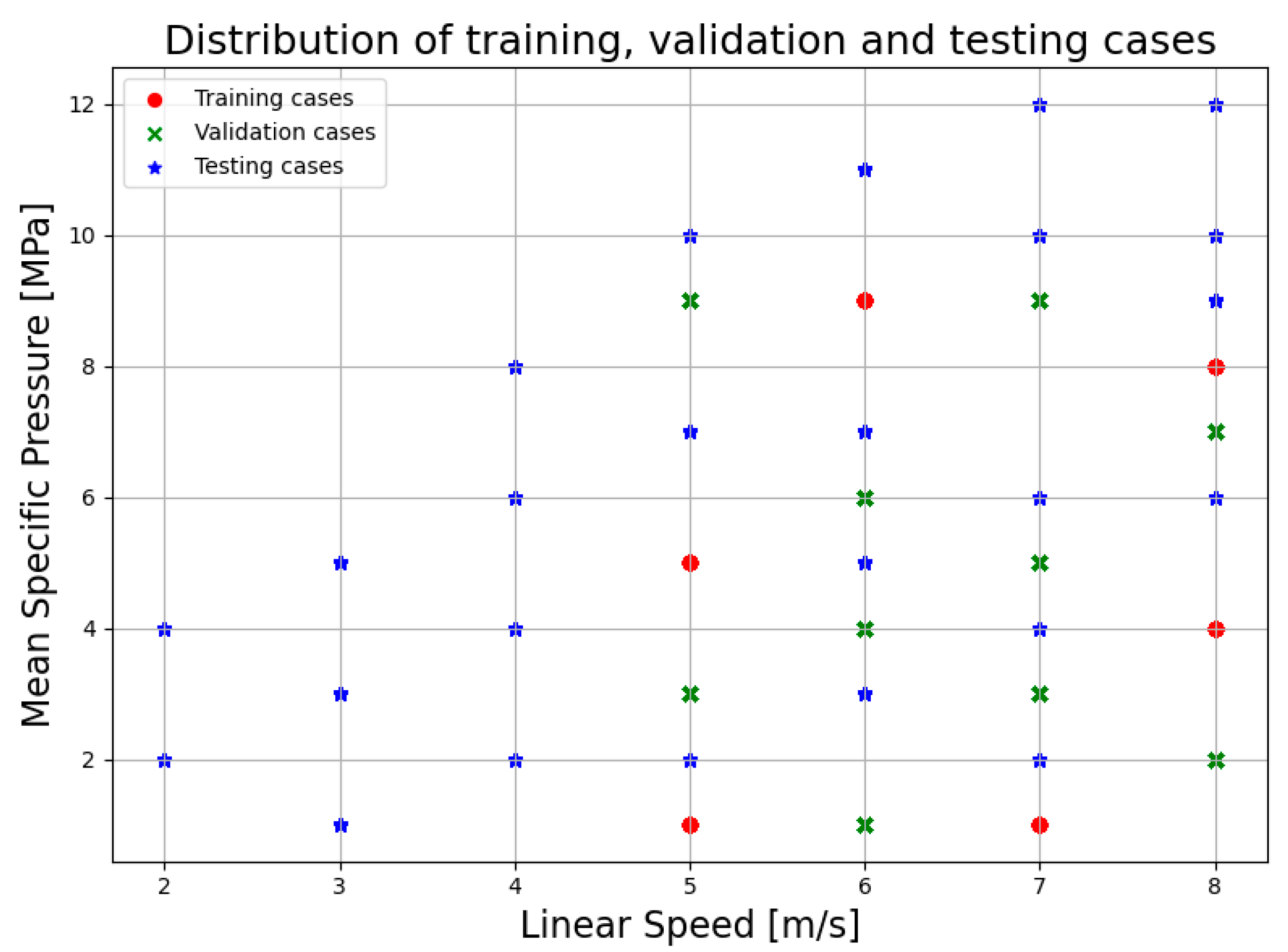
In this work, 41 simulation cases are carried out. These cases represent operating conditions exclusively within the hydrodynamic regime, as the focus of this work is on hydrodynamic contact conditions. Scenarios involving mixed friction are not considered and lie outside the scope of this study. Figure 1 represents the distribution of the load cases along the speed and load axes. As shown in Figure 1, the cases are divided into three categories: training cases (red), validation cases (green), and testing cases (blue). The training process utilises six cases (red) to supervise and guide the learning of the model parameters. Additionally, ten validation cases (green) are employed during training to assess the model’s capability and evaluate its overall prediction performance. Both training and validation cases cover a speed range from 5 to 8 m/s and a radial load from 0.45 to 4.05 kN, which corresponds to a mean specific pressure ranging from 1 to 9 MPa. The remaining 25 cases (blue) are designated as testing cases and are utilised after the training process is completed.
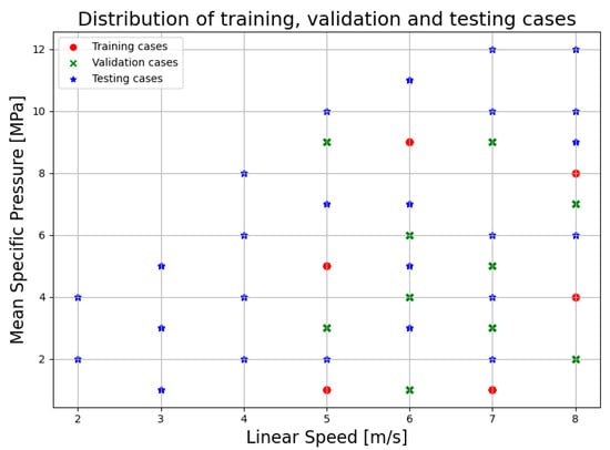
Figure 1.
Distribution of the simulation cases along the speed and load axes.
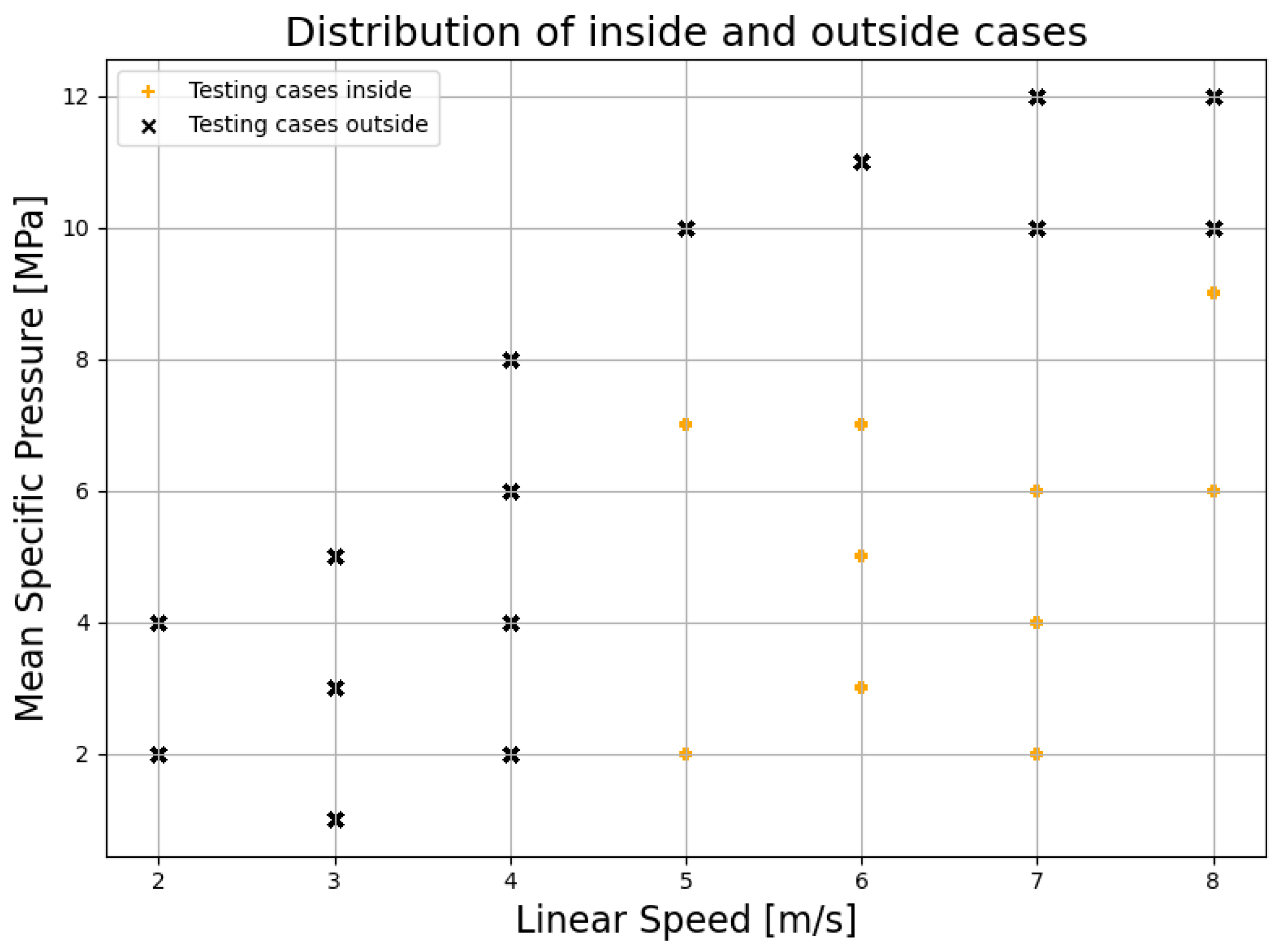
The testing cases are divided into two categories, as shown in Figure 2. The first category, called ‘inside testing’, involves assessing the model using cases within the defined load and speed ranges. Both the validation cases and the inside testing cases fall under the same category, encompassing a pressure range of 2 to 9 MPa and a speed range of 5 to 8 m/s. The only difference between them lies in their purpose for model evaluation: validation is used to assess the model during training after each epoch, while testing takes place after the model has been fully trained. The second category, referred to as ‘outside testing’, evaluates the model with cases that fall outside these specified ranges. This testing strategy examines how the model handles input data outside the training range, as well as its generalisation capability for cases beyond the training range.
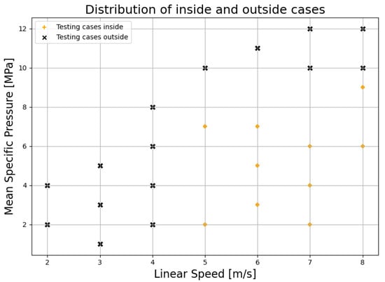
Figure 2.
Distribution of the inside and outside testing cases along the speed and load axes.
2.2. PINN Framework
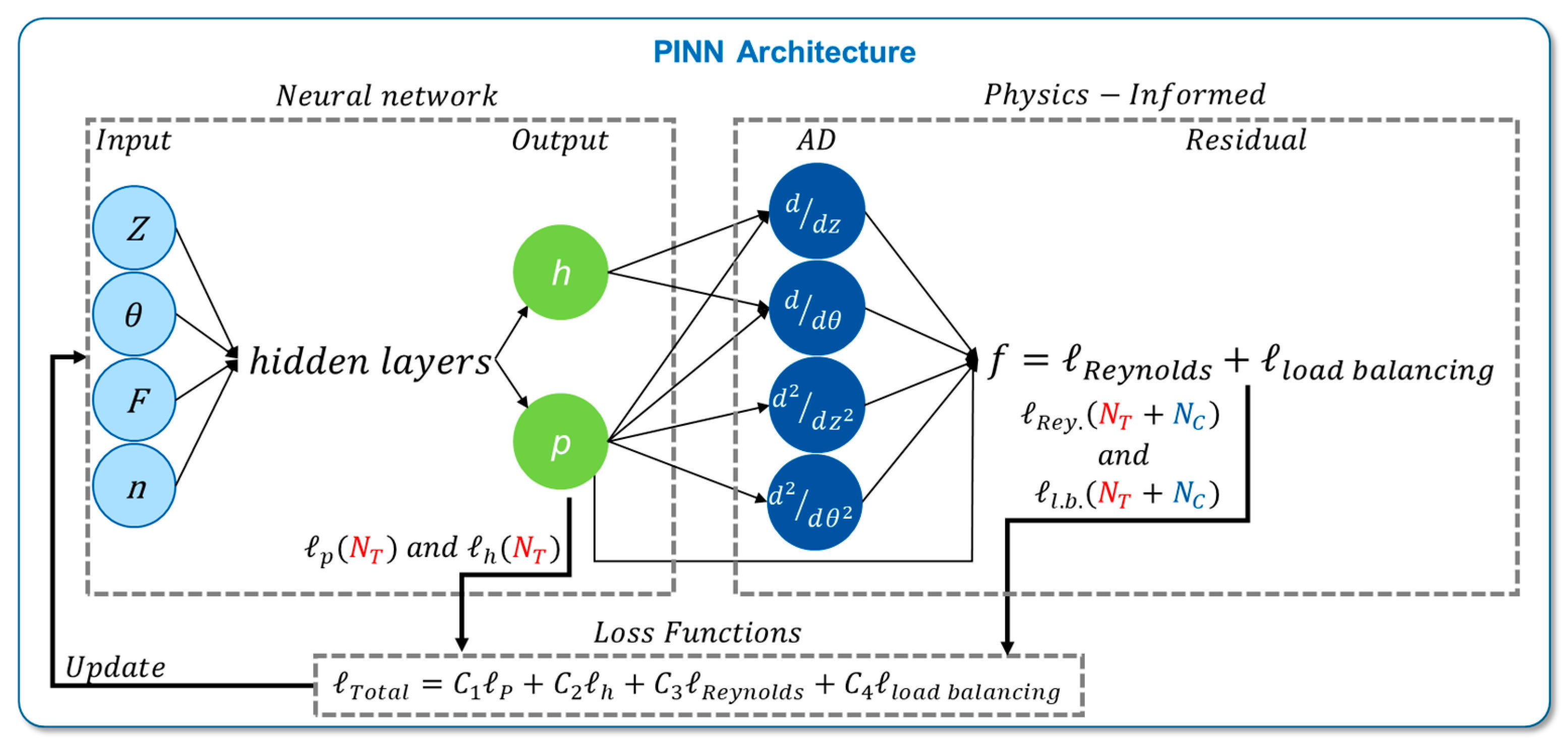
The PINN framework used to develop a real-time model for predicting hydrodynamic pressure and film thickness distribution in radial plain bearings is illustrated in Figure 3. The framework comprises two main components: a neural network block on the left-hand side and a physics-informed block on the right-hand side. The purpose of the neural network is to approximate the solutions p(θ, z) and h(θ, z). A standard Feedforward Neural Network (FF-NN) is utilised within this PINN framework for this purpose. The points used to train this framework comprise two different datasets: the training points (NT) and the collocation points (NC), which are defined as specific points where the PINN is trained to satisfy the governing physical equations, as shown in Figure 3. This is discussed in detail in Section 2.2.3.
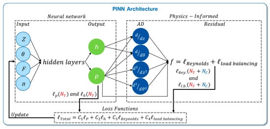
Figure 3.
PINN framework structure for real-time prediction of hydrodynamic pressure (p) and film thickness (h) distribution in radial plain bearings. The framework incorporates the axial (z) and circumferential (θ) directions, radial load (F), and rotational speed (n), as well as training points (NT) and collocation points (NC). Residuals (f) and loss functions (l) are used to guide model training.
The inputs to the network consist of vectors representing the radial load (F) and rotational speed (n) of the bearing, from which the sliding speed and specific pressure are derived. These inputs can also be captured by commonly available sensors in most applications. The network also receives the bearing HD mesh intervals in the θ- and z-directions, which correspond to the circumferential and axial directions, respectively. They are fed into a neural network with four hidden layers, each containing 256 neurons, utilising the ReLU (Rectified Linear Unit) activation function [46]. To avoid overfitting due to the high number of neurons, a dropout rate of 0.3 was implemented in the model. The presented framework adopts a different approach compared to models in the literature (see Table 1), which typically use fewer neurons and a greater number of layers due to the challenges associated with dealing with large domains. Therefore, an extensive study of all these parameters would need to be conducted to make reliable statements about computational efficiency; however, this is beyond the scope of this work. In contrast to the models in the literature, our model utilises a deeper architecture with more neurons per layer, as recommended for large domains by Moseley [48]. This design choice eliminates the need for a pre-training phase that focuses solely on the unsupervised, data-driven component aimed at balancing the physics loss, as recommended by Chen et al. [57].
The output layer consists of two neurons: one corresponding to the predicted p(θ, z), which uses the sigmoid activation function, offering advantages such as ensuring output values are bounded between 0 and 1, making it suitable for probabilities [41], and the other corresponding to the h(θ, z), which employs the softplus activation function [58]. The softplus function provides a smooth approximation to the ReLU function and ensures that the output remains positive, which is essential for representing physical quantities like film thickness [58]. Once the predictions p(θ, z) and h(θ, z) are obtained, the loss for both predictions is calculated using only the training points (NT), as shown in Figure 3. The loss function employed in this framework is discussed in Section 2.2.1.
The second block of the PINN framework, as shown in Figure 3, is the physics-informed block. The purpose of this block is to calculate the residuals f, which require the derivatives of the outputs concerning the inputs. This can be conveniently accomplished using Automatic Differentiation (AD) [41]. AD capabilities are commonly found in deep learning frameworks [59]. By employing AD in this study, the need for symbolic derivations or numerical discretisations to compute the derivatives of the Reynolds equation, as presented in Equation (1), is eliminated for both spatial and temporal dimensions [41]. The parameters of the fully connected network are trained using gradient descent methods that rely on the backpropagation of the loss function [41,59]. The residual f is determined in the presented framework using both the training points (NT) and the collocation points (NC), similar to the approach presented by Rom in his work [36].
The total loss L consists of two components: the data loss Ldata, which accounts for the training points on the boundaries of the domains, and the residual loss f, which captures the PDE residual and the load balancing constraints, as presented in Equations (2) and (3). In this work, the Mean Squared Error (MSE) is utilised to define the loss function. The specific loss functions employed are detailed in Section 2.2.1, while the training strategy, including data scaling and loss balancing, is described in Section 2.2.2. The training points used in this framework are explained in Section 2.2.3.
2.2.1. Loss Functions
For this framework, four custom loss functions for specific outputs are defined and utilised, all of which are based on the MSE. The first two loss functions represent the data loss, reflecting the supervised learning component of this framework, as shown in Equations (4) and (5). and represent the training errors for the hydrodynamic pressure and oil film thickness, respectively, associated with the data loss. C1 and C2 are the weight values assigned to these training errors. Here, NT denotes the number of training points in the θ- and z-directions for the training domains used, while pT and pP represent the true values of pressure and the predicted pressure, respectively, in the θ- and z-directions.
The residual loss f is represented by two loss functions. The first captures the PDE residual , which represents the Reynolds equation in a simplified form, as presented in Equation (6). The simplifications made include steady-state flow with no squeeze film action and the assumption that only one surface is in motion. These assumptions were considered when conducting the EHD simulations. In Equation (6), C3 represents the weight value assigned to the PDE residual, while NC denotes the collocation points, which are specific points where the PINN is trained to satisfy the governing physical equations. The definition and discussion of the collocation points can be found in Section 2.2.3.
The last loss function represents the load balancing between the applied load and the predicted load. Unlike the framework by Zhou [44], the load balance constraint is not integrated into the Reynolds equation but instead used as a separate load function. These functions are crucial for managing the physical constraints of film thickness and the surface elastic deformation due to the hydrodynamic pressure. Here, fT and fP denote the values of the applied force and the predicted force, respectively. The applied force is a known global input related to the external load, while the predicted force is obtained by integrating the predicted pressure field over all 1944 domain points in each case, resulting in a single global force value per case. This is associated with C4 as the weight value assigned to this loss function. Additionally, ND represents the number of domain points in this framework, which amounts to 1944 data points, corresponding to the discretisation of the HD mesh.
2.2.2. Training Strategy
The training objective is to minimise the training error associated with the neural network, along with the error related to the PDE residuals and the constraints implemented in this framework. For initialising the parameters of the neural network, specifically their weights and biases, Kaiming uniform initialisation (also known as He initialisation) [60] is employed, which is suitable for the ReLU activation function. The optimisation of these parameters is subsequently carried out using the Adaptive Moment Estimation (Adam) algorithm with a dynamic learning rate starting from η = 10−3. Based on the state of the art, Adam is a widely adopted optimiser used in PINNs [41,42,46]. Its efficiency in managing large-scale problems and low memory overhead make it particularly well-suited for these applications [46]. As recommended by the state of the art, input data should be normalised to improve the convergence speed of the training process and enhance the overall performance of the neural network [61]. In this framework, the input data is normalised to a range of 0 to 1 using simple scaling based on the maximum values. This scaling is applied only during the neural network block; therefore, when calculating the Reynolds equation residual or the load balancing constraints, the data are not scaled or normalised.
A significant challenge in the development of the PINN framework is effectively balancing the four different loss terms it encompasses. In this framework, rather than manually estimating the importance of each loss term, the self-adaptive loss balancing method presented by Xiang is employed [62]. This method defines weights (C1, C2, C3, C4) that automatically adjust during training to ensure a proper balance among all losses, with a Gaussian function used to link each loss to its corresponding weight, facilitating the adjustment process [62].
2.2.3. Training Points
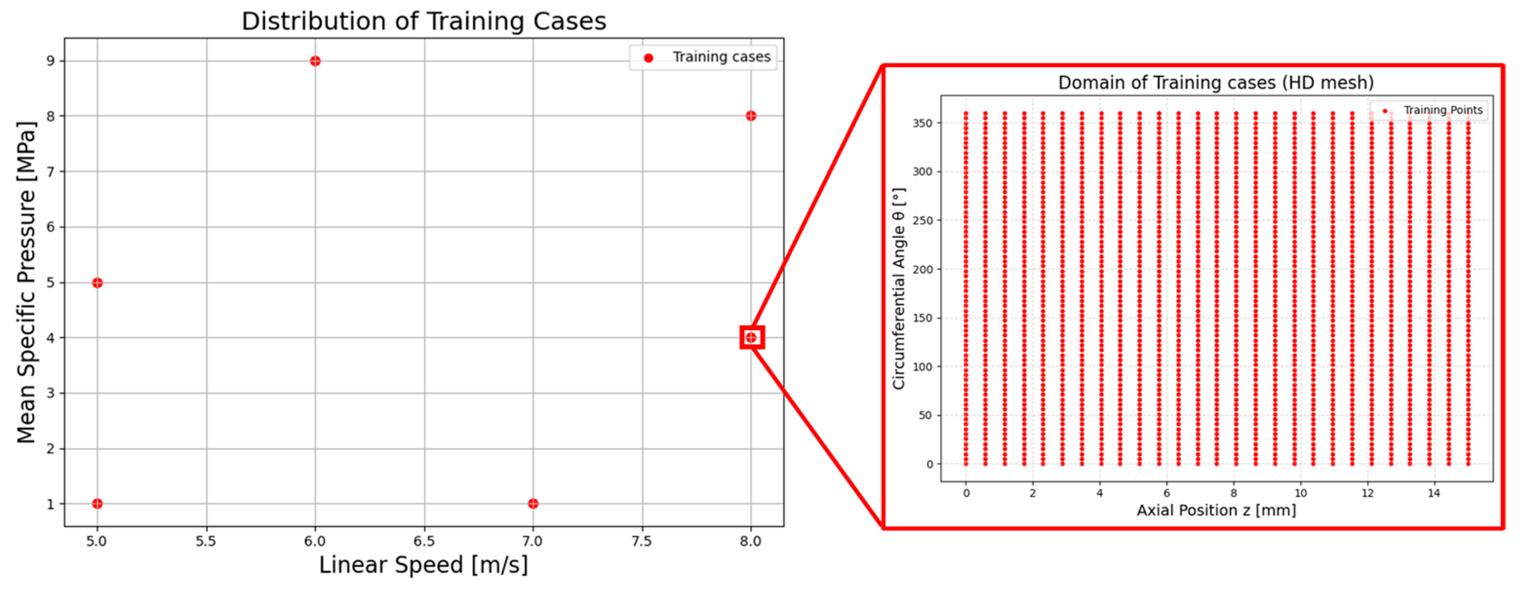
To train a model using the PINN framework, two different datasets are used during the training phase: the six training cases presented in Section 2.1.2 and the collocation points. The training points (NT) represent the supervised component of this framework, with each training case consisting of 1944 training points corresponding to the hydrodynamic mesh nodes (see Section 2.1.1), as shown in Figure 4. This means the total number of training points used for supervised learning is 11,664, calculated as 1944 domain points per case across 6 training cases.
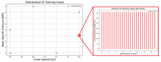
Figure 4.
Distribution of the training cases and their corresponding training point (NT) distribution.
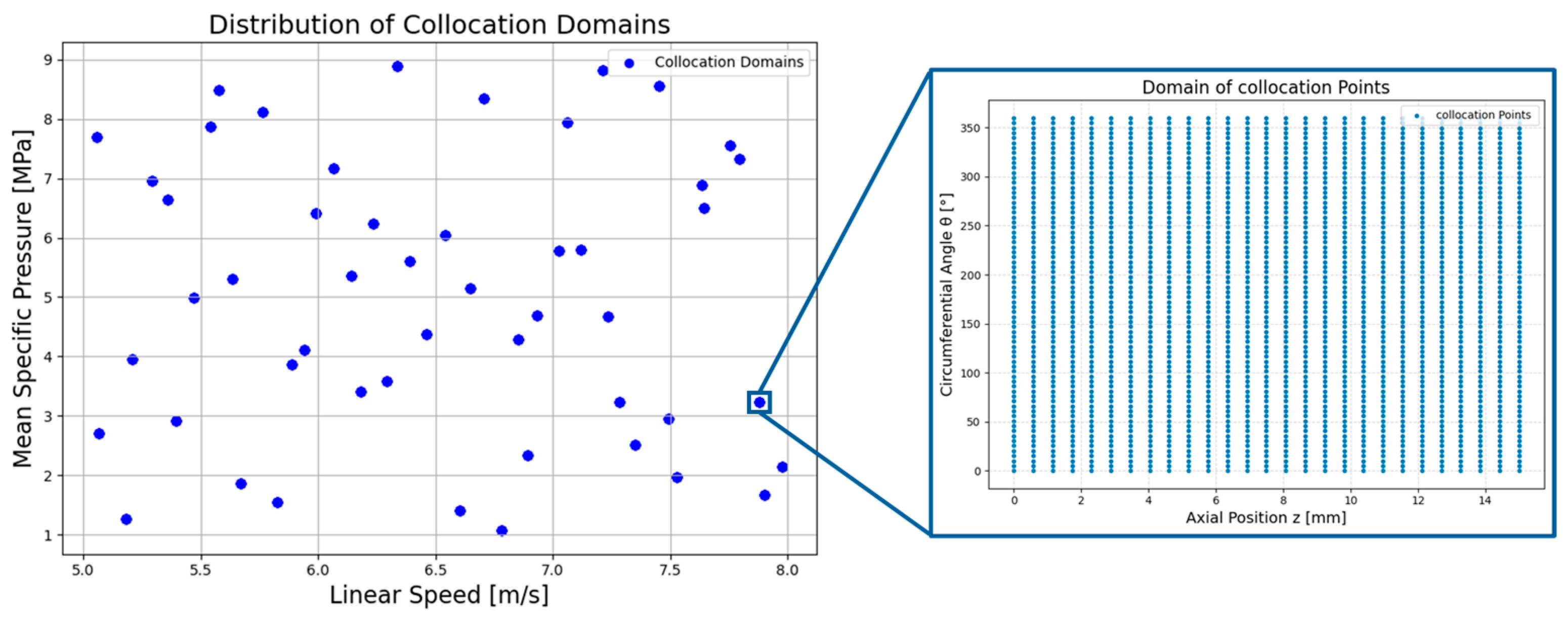
In this work, collocation points (NC) are utilised to enforce the governing physical equations within the domains, representing the unsupervised component of the PINN framework. These are specific points in the training domain where the model is trained to satisfy the governing equations, including the Reynolds equation and the load balance constraint. A total of 50 collocation domains are generated within the boundaries defined by the training data, which range from 5 to 8 m/s for speed and from 0.45 to 4.05 kN for radial load, corresponding to a mean specific pressure ranging from 1 to 9 MPa. To ensure a uniform and representative distribution across this multi-dimensional space for collocation domains, Latin Hypercube Sampling (LHS) is employed. LHS is a stratified sampling technique that ensures that the entire range of each variable is well covered without clustering, which enhances training stability and physical accuracy [63]. Each domain contains 1944 collocation points generated using uniformly distributed sampling, similar to the training point distribution, to ensure better stability. This means the total number of collocation points used for unsupervised learning is 97,200, calculated as 1944 domain points per case across 50 collocation domains. Figure 5 shows the distribution of the collocation domains and their corresponding collocation point distributions.
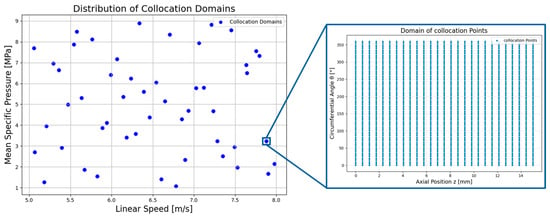
Figure 5.
Distribution of the collocation domains and their corresponding collocation points (NC) distributions.
3. Results and Discussion
This chapter discusses the validation and testing of the developed model using the PINN framework for real-time prediction of hydrodynamic pressure and film thickness distribution in radial plain bearings. The validation and testing are based on the data from the numerical simulations described in Section 2.1. This section begins in Section 3.1 by presenting the model behaviour during the training process, including the validation accuracy. Section 3.2 follows with an examination of the model’s behaviour using a testing strategy that evaluates performance both within and outside the training domain, as illustrated in Figure 2 and discussed in Section 2.1.2.
3.1. Model Behaviour and Validation Throughout Training
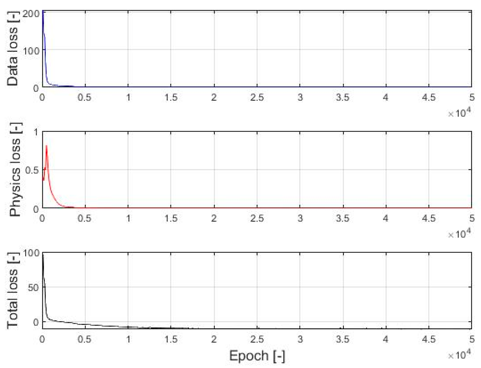
The model behaviour during the training process can be described using the training loss history, which demonstrates how the model adapted to the training and collection points, as well as the outcomes from the validation points. The training loss history for the training duration is shown in Figure 6. Figure 6 demonstrates that the model learns consistently, with the supervised loss (blue line) initially very high and quickly dropping within the first few hundred epochs. The physics loss (red line) starts relatively low compared to the supervised loss due to gradient magnitude differences and decreases slowly, exhibiting very little fluctuation. This behaviour indicates that the model satisfies the physical laws implemented. The total loss (black line) represents both the supervised loss and physics loss; it starts high and decreases over the training period. The occurrence of negative values in the total loss, resulting from overcompensation or adjustments aimed at minimising specific errors, is normal when employing a self-adaptive loss balancing method [62]. This is acceptable as long as the other losses remain positive, which is indeed the case with the model results [62]. The model takes between 40,000 and 60,000 epochs to be effectively trained. Although the loss values are already very low after approximately 30,000 epochs, continued training can still significantly improve the model’s predictive accuracy and stability. This helps reduce spectral bias, which is the tendency of neural networks to learn smooth, low-frequency features more quickly than sharp, high-frequency details [48]. This issue can be further amplified by rescaling the input before it enters the physics-informed part of the framework, as rescaling can cause even low-frequency features to appear as high-frequency ones over larger domains, making them more difficult for the network to learn.
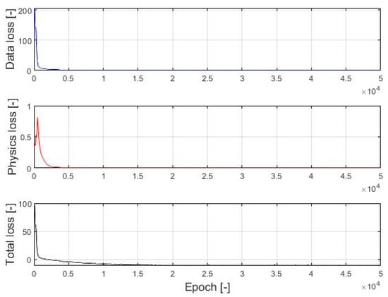
Figure 6.
Training loss history.
To assess the accuracy of its predictions compared to the true values, the model was validated using both the coefficient of determination (R2 score) and the Root Mean Square Error (RMSE). In the case of validation during the training process, the overall validation accuracy for pressure and film thickness distribution after 50,000 epochs achieves an R2 scores of 0.9985 and 0.9994, respectively. These values represent the overall accuracy of all 10 validation data points. The deviation between the true values and the model predictions, although very small and potentially negligible, may be influenced by the distribution as well as the number of collocation domains. The individual R2 scores, RMSE values, and true and predicted values, along with percentage errors for peak hydrodynamic pressure and minimum oil film thickness, are presented in Table 3.

Table 3.
Results of the model validation.
For hydrodynamic pressure, the R2 values range from 0.9683 to 0.9970, and the RMSE values range from 0.104 to 0.399 MPa, indicating a high level of correlation between the predicted and true values. The overall peak pressure percentage error across all cases is 2.32%, with a maximum error of 11% in case 8. Although this error appears significant, it is primarily due to the small magnitude of the true peak pressure (2.37 MPa) compared to the predicted value of 2.64 MPa. In terms of oil film thickness, the R2 values are consistently high, ranging from 0.9972 to 0.9999, and the RMSE values are very small, ranging from 0.127 to 0.543 μm, suggesting excellent predictive accuracy. The overall percentage error in the prediction of minimum oil film thickness across all cases is 3%, with a maximum error of 10% observed in Case 5. Although the error may seem significant, it is primarily due to the small magnitude of the true film thickness, with the absolute deviation reaching only 0.553 μm.
3.2. Post-Training Evaluation of Real-Time Model Behaviour
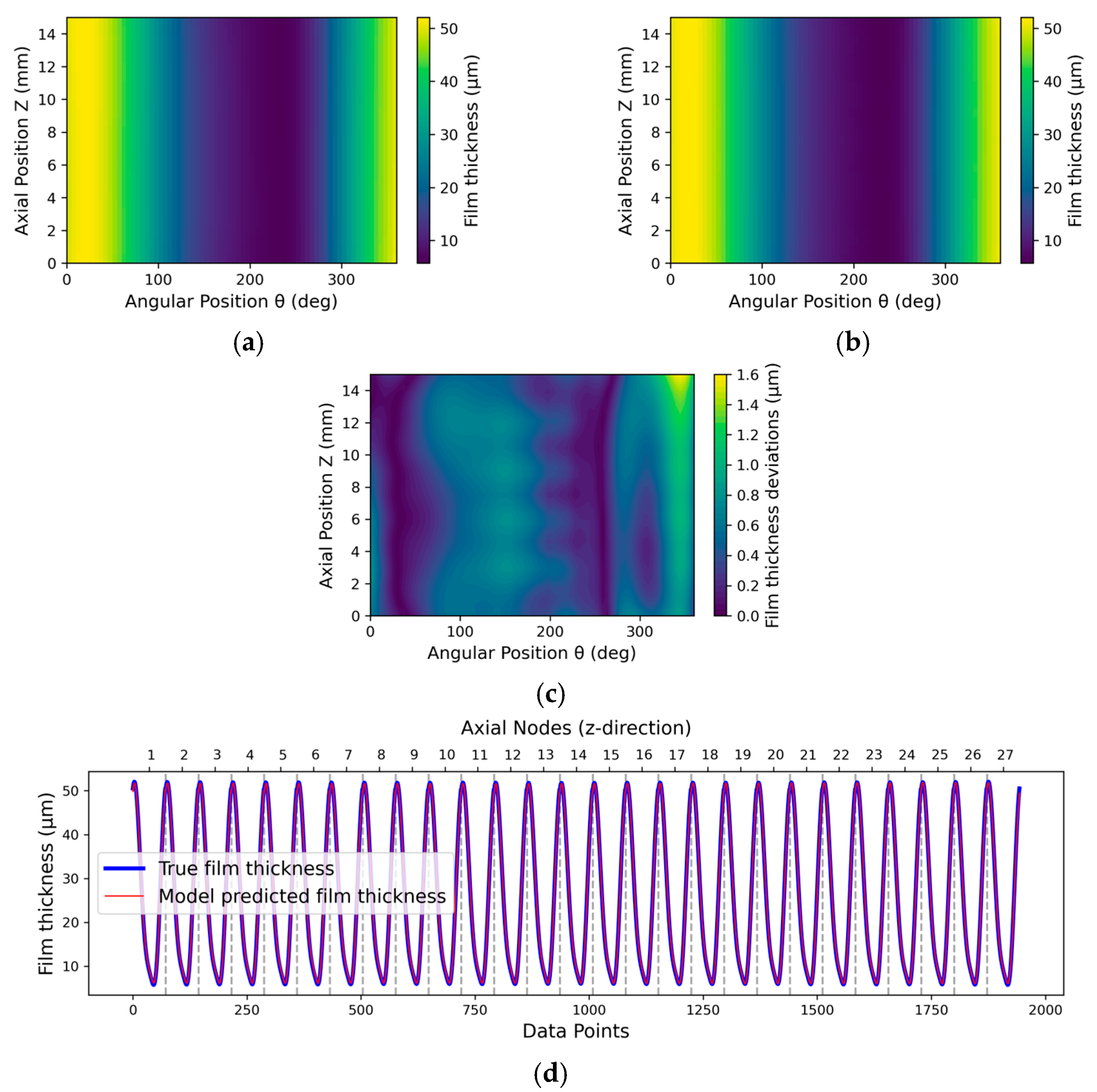
As mentioned in Section 2.1.2, the testing strategy for the real-time model consists of two categories: ‘inside testing’, which assesses the model using cases within defined load and speed ranges, and ‘outside testing’, which evaluates cases beyond these ranges. As mentioned in Section 3.1, both the R2 score and the RMSE are used to test the model and assess the accuracy of its predictions compared to the true values. Although these two evaluation methods are state-of-the-art techniques for assessing a machine learning model, they can sometimes lead to misleading conclusions. For instance, a high R2 does not guarantee that the model’s predictions are unbiased, as it can be influenced by the distribution of the data. Similarly, RMSE is scale-dependent and can be skewed by whether the true values are generally high or low, which may misrepresent the model’s actual performance. Thus, in this work, a graphical approach is introduced alongside the use of the true error of peak hydrodynamic pressure and minimum oil film thickness. The graphical approach visually evaluates the deviation between the true values and the model predictions for every point in the data domain by flattening the classic 2D domain into 1D. Figure 7 explains the process of flattening the classic 2D data domain into a 1D data domain.
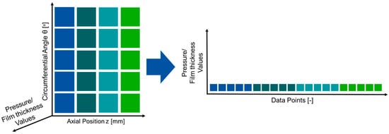
Figure 7.
Flattening the classic 2D data domain into 1D data domain.
3.2.1. Inside Testing
As stated in Section 2.1.2, the predictions of the real-time model are evaluated using 10 test cases within its training domain. The training domain encompasses a pressure range of 2 to 9 MPa and a speed range of 5 to 8 m/s. The individual R2 scores, RMSE values, and true and predicted values, along with percentage errors for peak hydrodynamic pressure and minimum oil film thickness, are listed in Table 4. The table summarises the prediction results of the evaluation metrics for hydrodynamic pressure and oil film thickness of the real-time model. The predictions require less than one second for each testing case, while the model demonstrates strong predictive performance for both hydrodynamic pressure and oil film thickness.

Table 4.
Evaluation of predictions of the real-time model within its training domain.
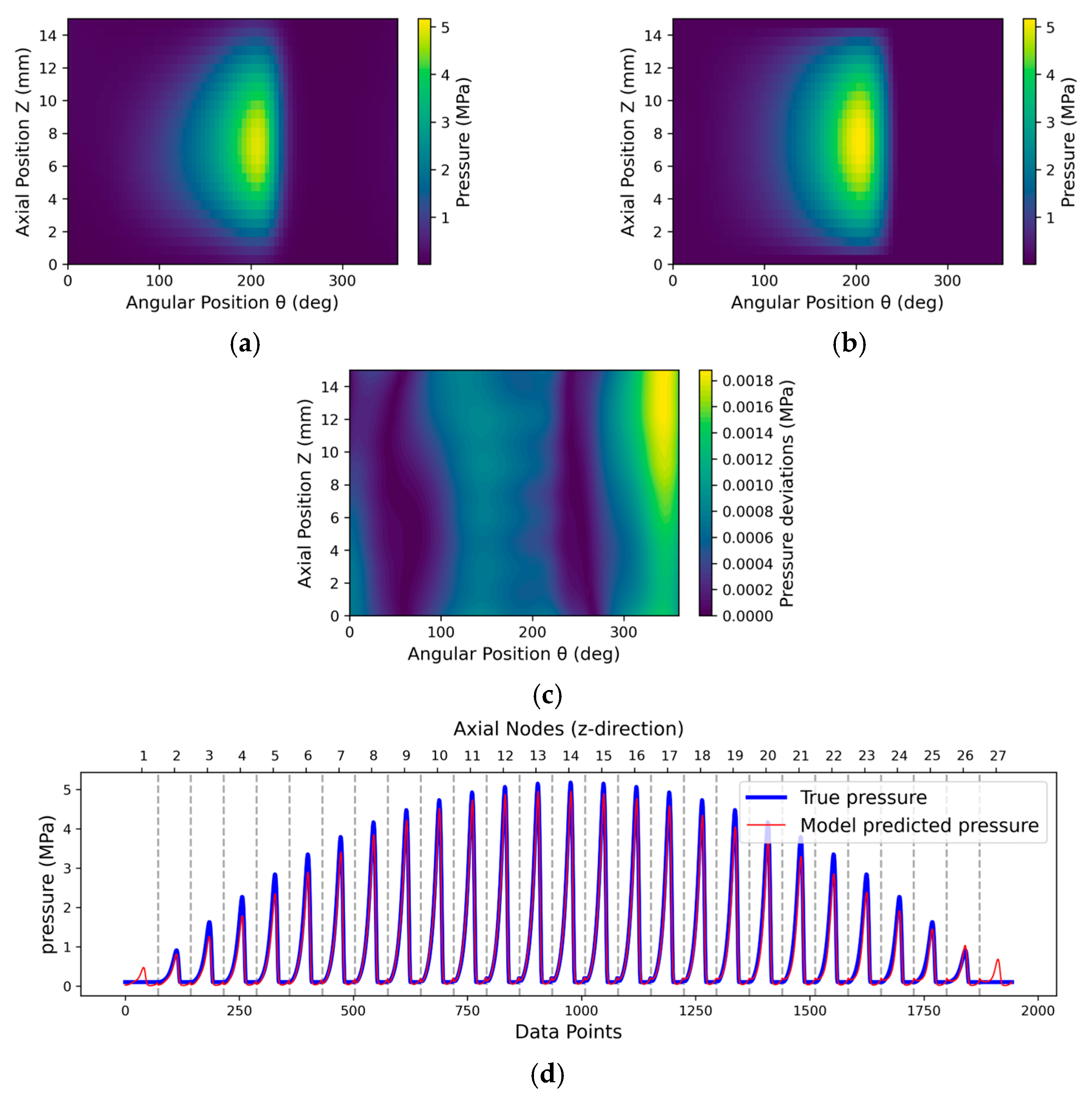
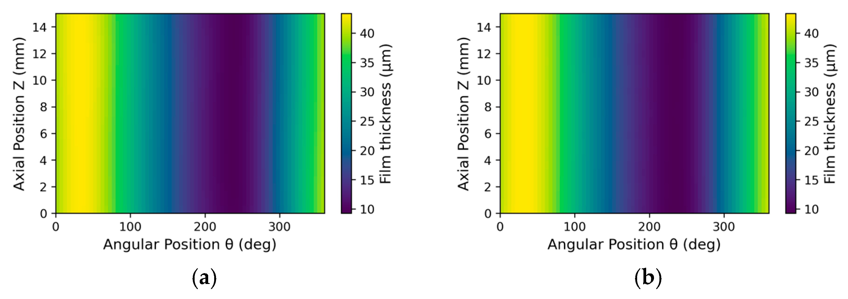
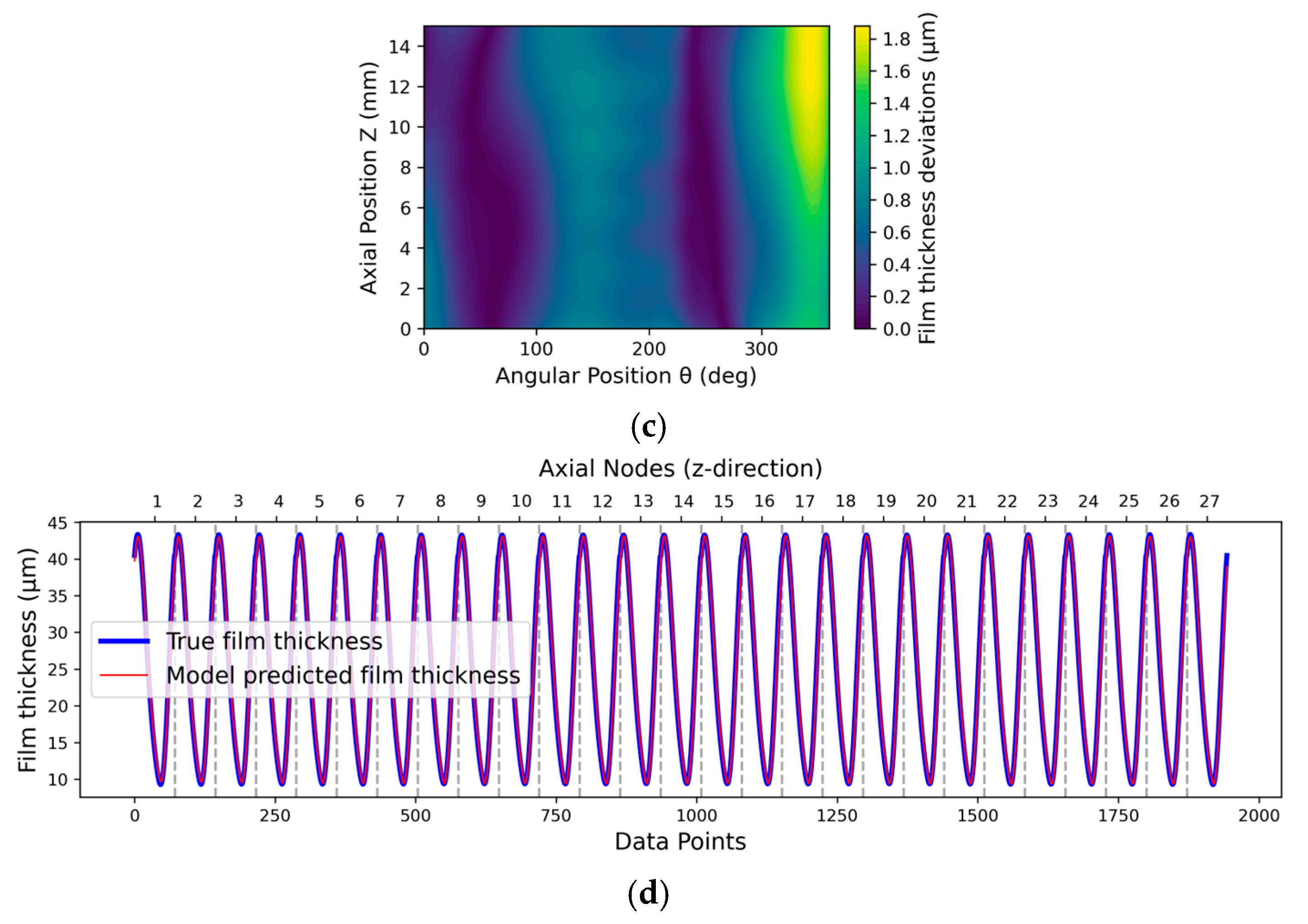
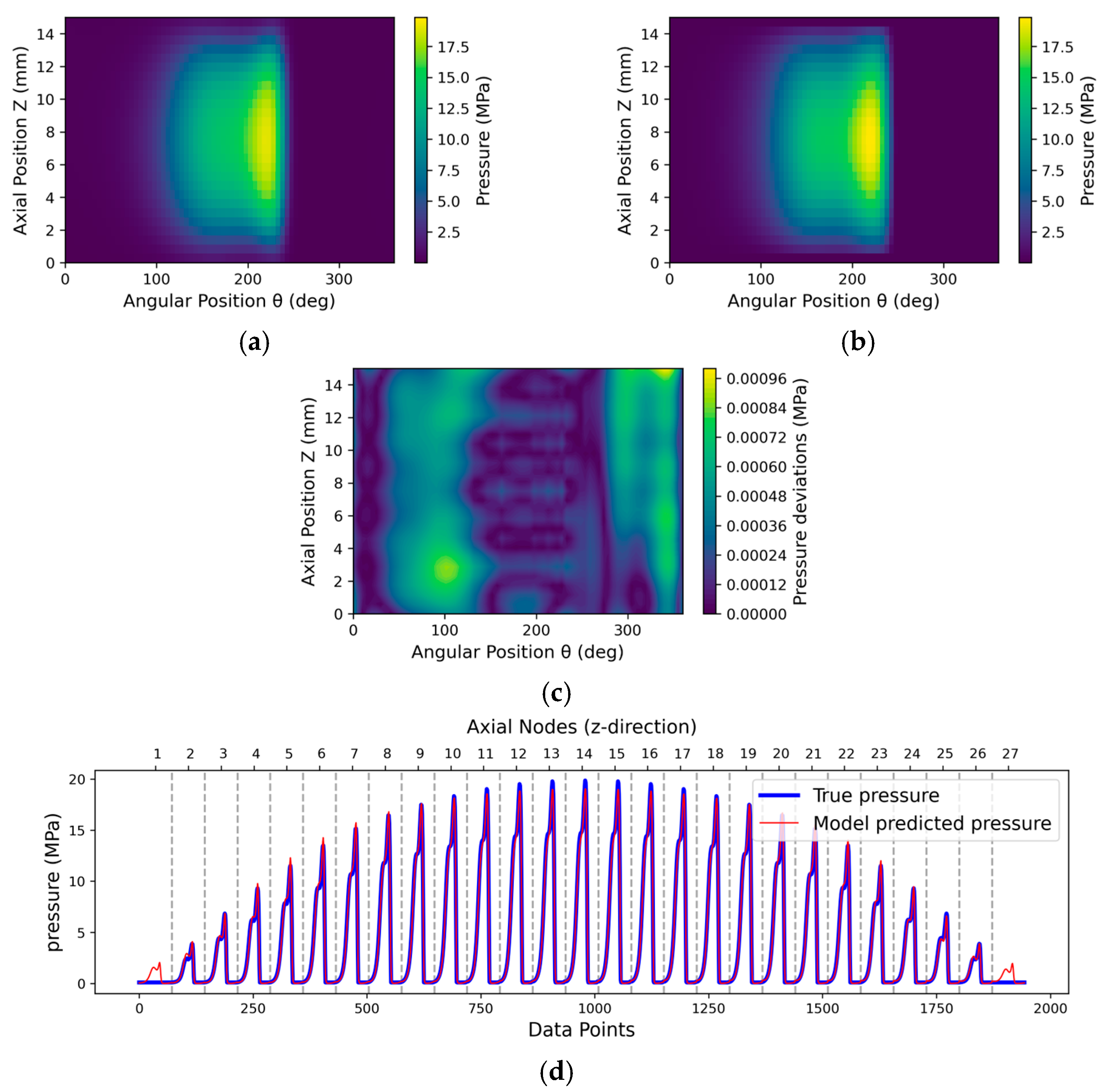
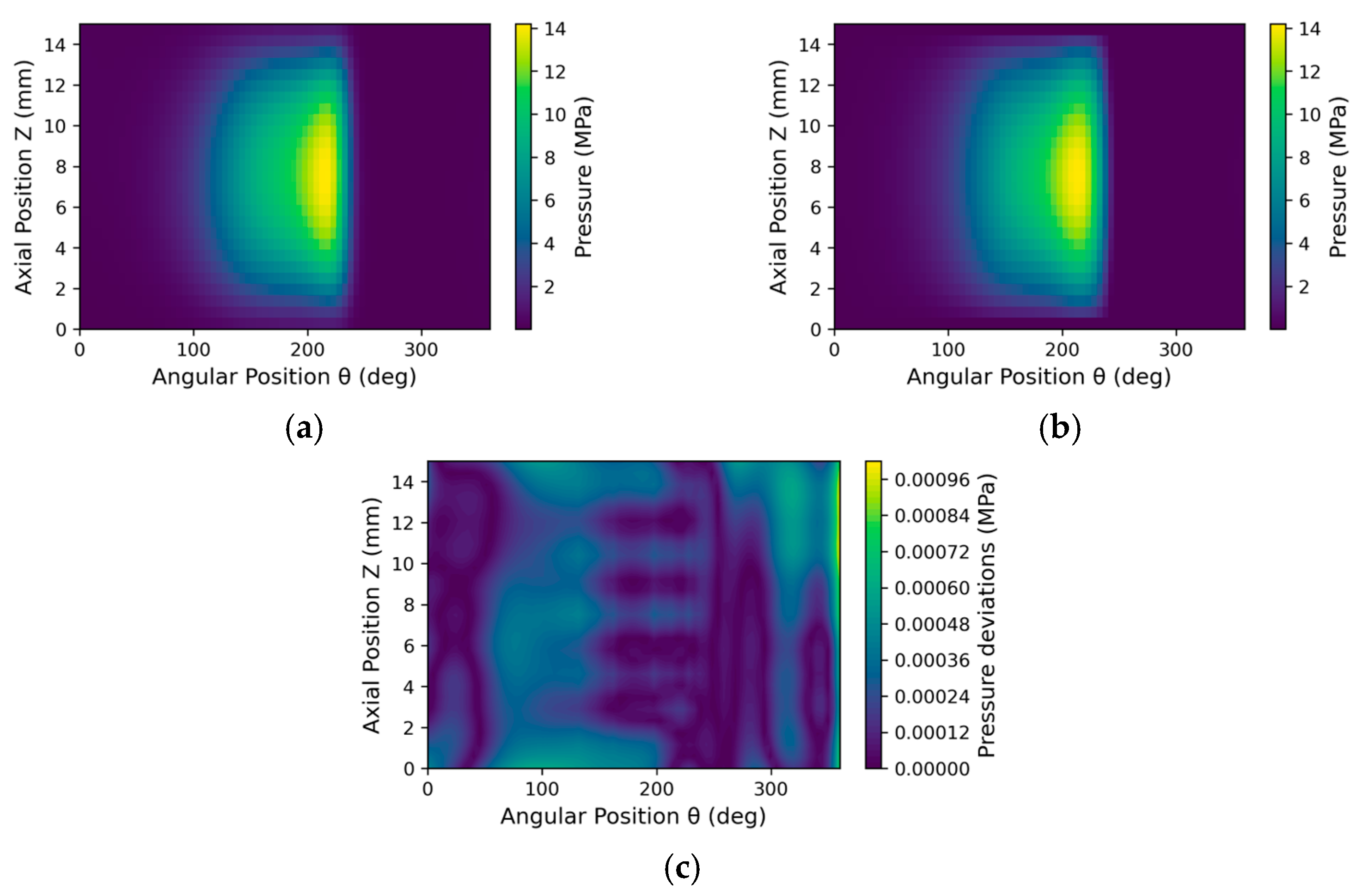
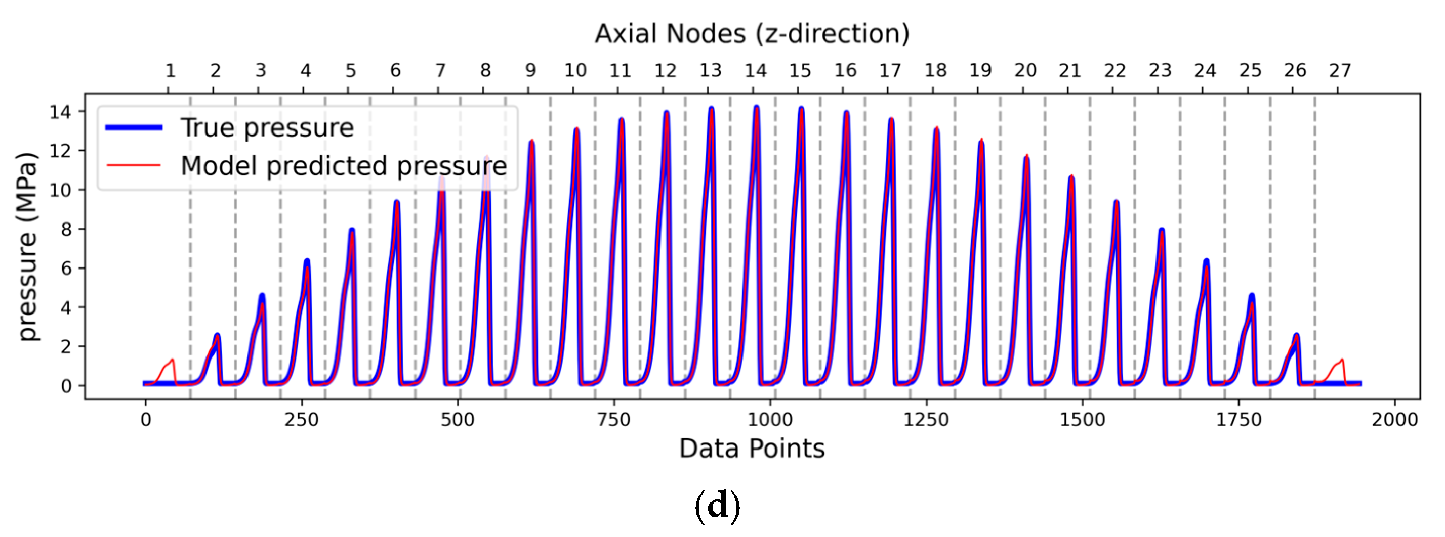
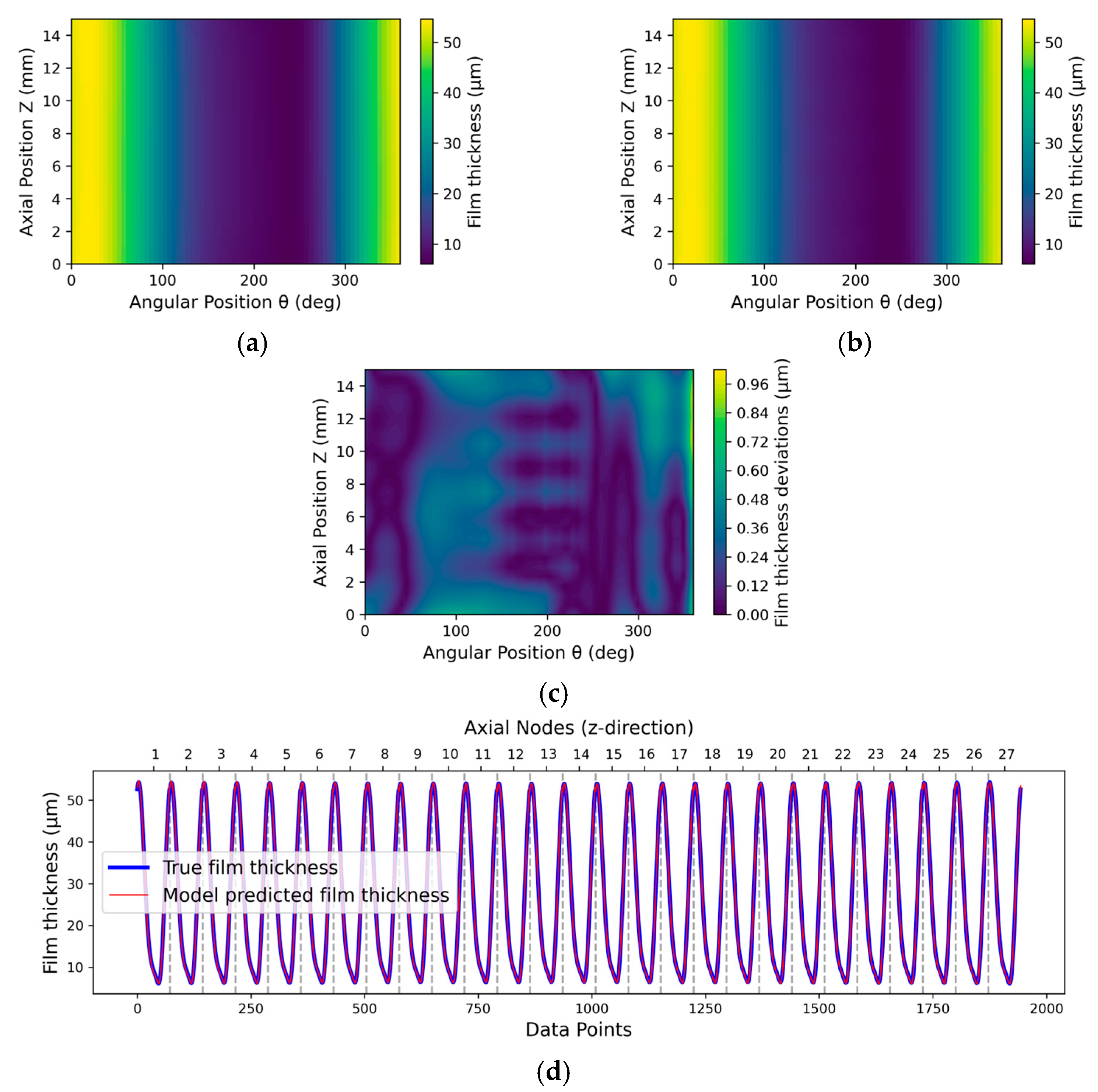
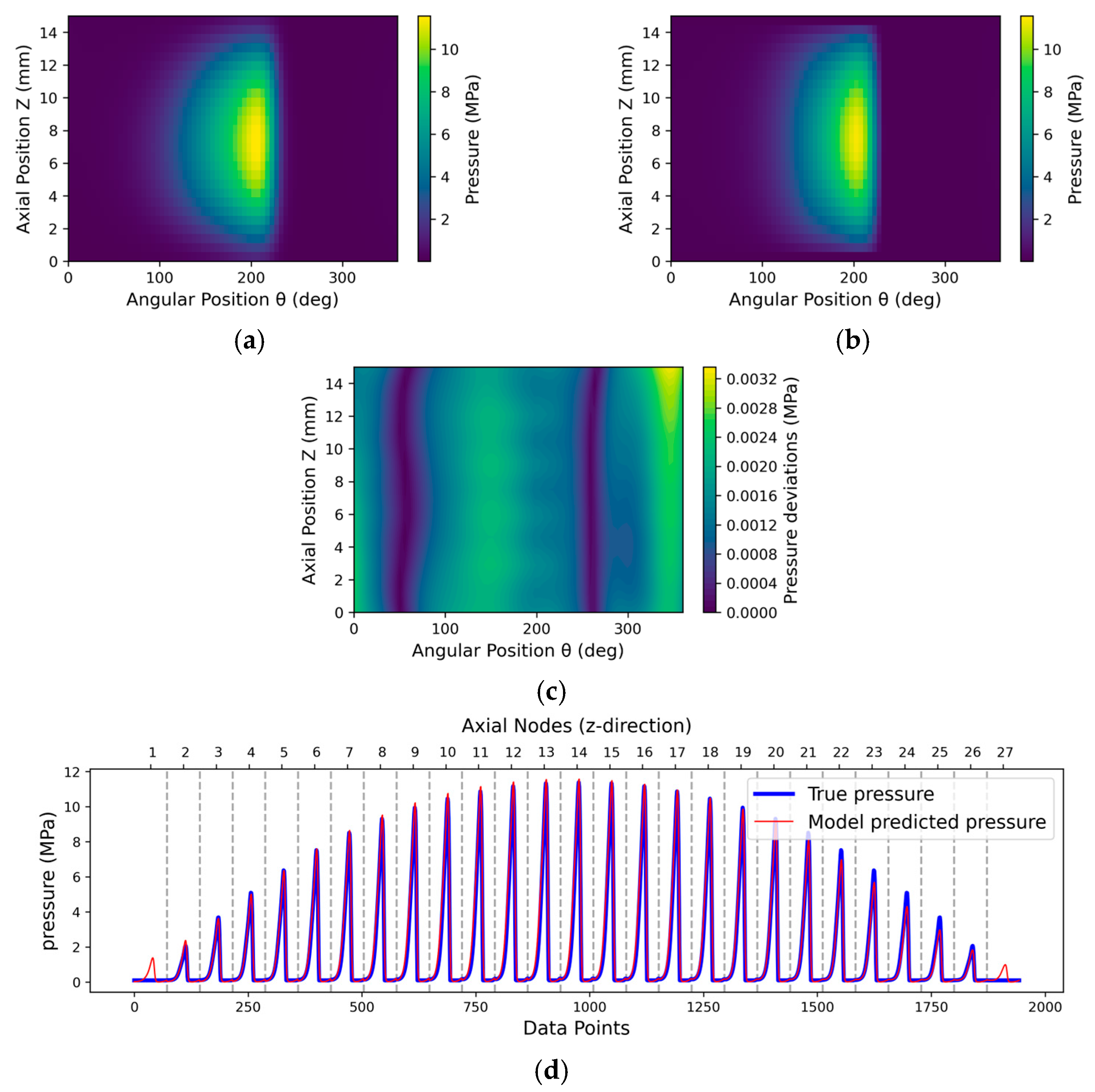
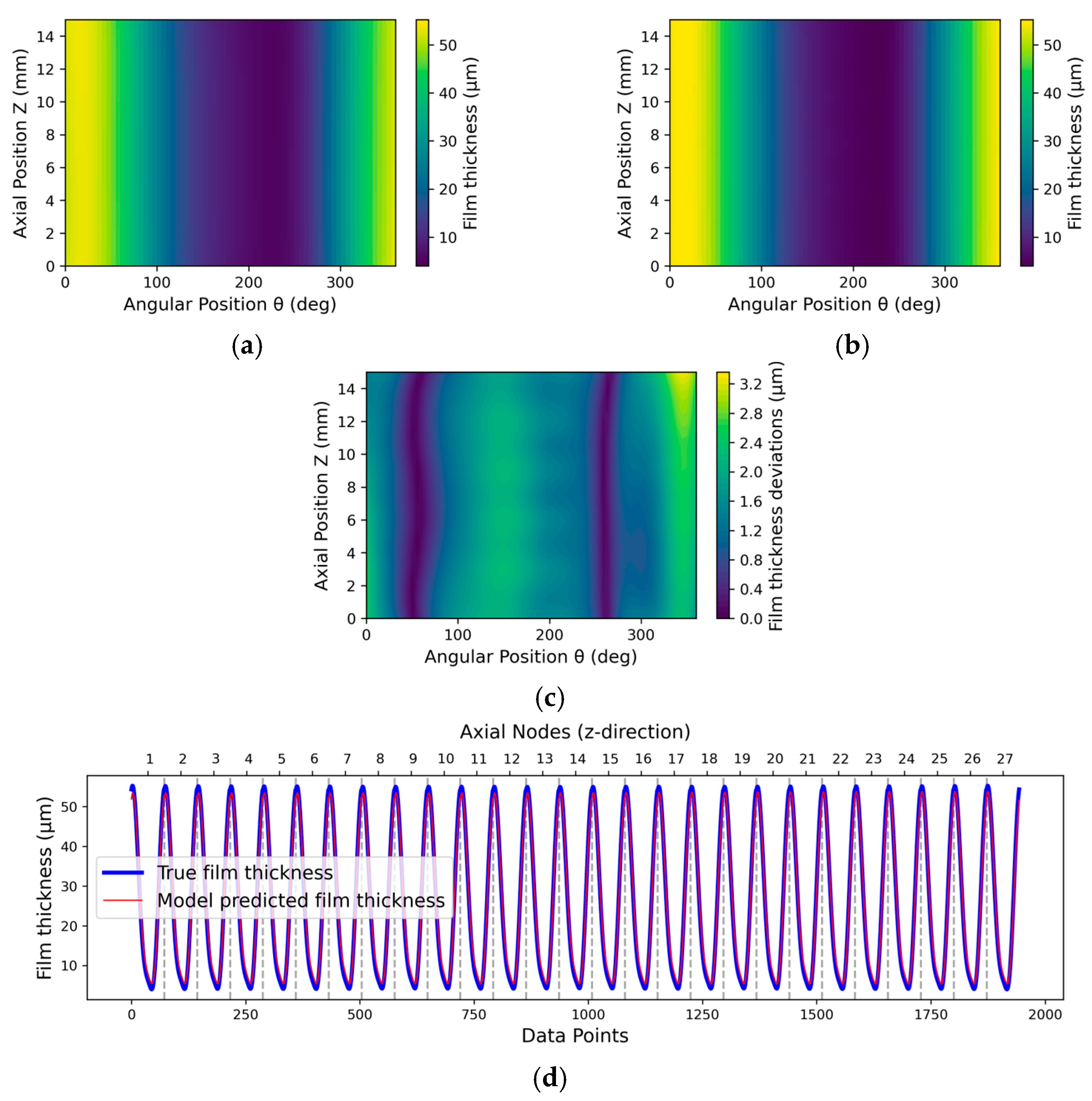
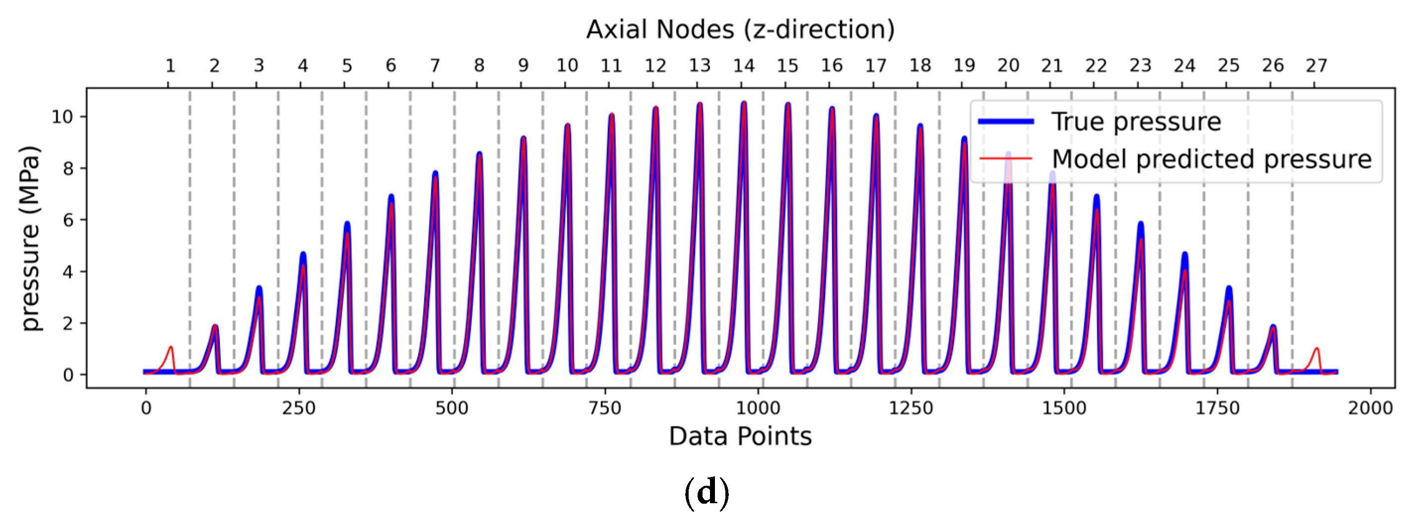
The model achieves R2 scores between 0.9768 and 0.9967 for hydrodynamic pressure and between 0.9964 and 0.9999 for oil film thickness, as shown in Table 4. Corresponding RMSE values range from 0.165 to 0.339 MPa for pressure and from 0.148 to 0.718 μm for film thickness. The overall percentage errors for peak pressure and film thickness across all cases are 1.37% and 1.96%, respectively. The maximum errors recorded are 4.33% for pressure in Case 7 and 5.2% for oil film thickness in Case 8. In absolute terms, these maximum percentage errors correspond to only 0.22 MPa for pressure and 0.263 μm for film thickness. According to Table 4, there is no clear correlation between the deviation and either the load or the RPM. Additionally, since the validation cases can also be considered inside testing cases, there is no clear correlation between the deviation and either the load or the RPM. However, when the true values are very small, the percentage error tends to increase noticeably. The highest deviation occurs in Cases 7 and 8, which have the lowest R2 scores and some of the highest RMSE values, along with significantly higher absolute error values for peak hydrodynamic pressure and oil film thickness. These results are presented in Figure 8 and Figure 9 for Case 7 and Figure 10 and Figure 11 for Case 8. These figures show the 2D distributions of both predicted and true values, along with the 2D deviation between them. They also include a comparison of these values in a 1D flattened format for hydrodynamic pressure and oil film thickness, respectively. The figures demonstrate a strong qualitative agreement between the predicted and true distributions of hydrodynamic pressure and oil film thickness, despite limitations in capturing peak pressure and challenges in predicting the exact minimum oil film thickness. The lowest deviation occurs in Case 6, which has the highest R2 score and one of the lowest RMSE values, along with significantly lower absolute error values for peak hydrodynamic pressure and oil film thickness. This case is presented in Figure 12 and Figure 13, which show a very good agreement between the predicted and true distributions of hydrodynamic pressure and oil film thickness. Notably, hydrodynamic pressure and oil film thickness show similar distributions of deviation despite having different physical units, as shown, for example, in Figure 8c and Figure 9c for Case 7 and in Figure 10c and Figure 11c for Case 8. This indicates their physical interdependence and shared sensitivities within the model, which could allow us in future work to focus on minimising the error of just one of these outputs to further improve overall prediction accuracy. While the 2D distributions of deviation vary from case to case, reflecting differences in operating conditions and model response, they consistently show that the most significant deviations do not occur in the loading zone of the bearing, around 200 degrees. This strengthens the model’s predictive reliability.

Figure 8.
Evaluation of the hydrodynamic pressure prediction for case 7 (inside testing): (a) the predicted values, (b) the true values, (c) 2D deviation between true and predicted values, (d) 1D comparison between true and predicted values.
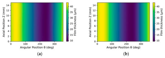
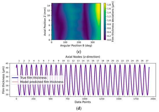
Figure 9.
Evaluation of the oil film thickness prediction for Case 7 (inside testing): (a) predicted values, (b) true values, (c) 2D deviation between true and predicted values, (d) 1D comparison between true and predicted values.

Figure 10.
Evaluation of the hydrodynamic pressure prediction for Case 8 (inside testing): (a) predicted values, (b) true values, (c) 2D deviation between true and predicted values, (d) 1D comparison between true and predicted values.
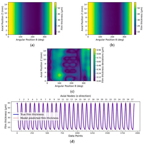
Figure 11.
Evaluation of the oil film thickness prediction for case 8 (inside testing): (a) the predicted values, (b) the true values, (c) 2D deviation between true and predicted values, (d) 1D comparison between true and predicted values.

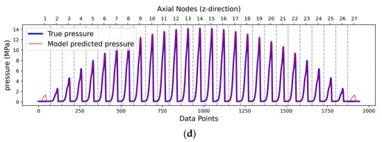
Figure 12.
Evaluation of the hydrodynamic pressure prediction for Case 6 (inside testing): (a) predicted values, (b) true values, (c) 2D deviation between true and predicted values, (d) 1D comparison between true and predicted values.

Figure 13.
Evaluation of the oil film thickness prediction for Case 6 (inside testing): (a) predicted values, (b) true values, (c) 2D deviation between true and predicted values, (d) 1D comparison between true and predicted values.
3.2.2. Outside Testing
The goal of outside testing is to evaluate the model’s predictions beyond its training domain to assess the model’s generalisation capability and validity range. In this work, the model was tested using 15 test cases outside its training domain, which defines a pressure range of 2 to 9 MPa and a speed range of 5 to 8 m/s, as shown in Figure 2. Since mixed friction was not the focus of this paper, only cases of operation in a fully hydrodynamic regime were used. The individual R2 scores, RMSE values, and true and predicted values, along with percentage errors for peak hydrodynamic pressure and minimum oil film thickness, are presented in Table 5. The model achieves R2 scores between 0.9724 and 0.9953 for hydrodynamic pressure and between 0.9819 and 0.9997 for oil film thickness, as shown in Table 5. Corresponding RMSE values range from 0.100 to 0.951 MPa for pressure and from 0.302 to 2.016 μm for film thickness. The overall absolute percentage errors for peak pressure and minimum film thickness across all cases are 4.88% and 12.31%, respectively. The maximum absolute errors recorded are 10.82% for pressure in Case 3 and 33.9% for oil film thickness in Case 2. In absolute terms, these deviations correspond to only 2.72 MPa for pressure and 1.349 μm for film thickness. As shown in Table 5, the deviation increases when the operating conditions deviate significantly from the training range. This is evident in Cases 1 and 2, which are the furthest from the training data and exhibit the highest prediction errors. The highest deviation occurs in Case 2, which has the lowest R2 score and one of the highest RMSE values, along with significantly higher absolute error values for peak hydrodynamic pressure and oil film thickness. Case 2 is presented in Figure 14 and Figure 15, which show the 2D distributions of both predicted and true values, along with the 2D deviation between them. They also include a comparison of these values in a 1D flattened format for hydrodynamic pressure and oil film thickness, respectively. The figures demonstrate a close qualitative agreement between the predicted and true distributions of hydrodynamic pressure and oil film thickness. The lowest deviation occurs in Case 7, which has two of the highest R2 scores of 0.9939 for hydrodynamic pressure and 0.9990 for oil film thickness, along with some of the lowest RMSE values of 0.197 MPa for hydrodynamic pressure and 0.497 μm for oil film thickness. Additionally, it shows significantly lower absolute error values of 0.58% for peak hydrodynamic pressure and 4.80% for oil film thickness. This case is presented in Figure 16 and Figure 17.

Table 5.
Evaluation of predictions of the real-time model outside its training domain.

Figure 14.
Evaluation of the hydrodynamic pressure prediction for Case 2 (outside testing): (a) predicted values, (b) true values, (c) 2D deviation between true and predicted values, (d) 1D comparison between true and predicted values.
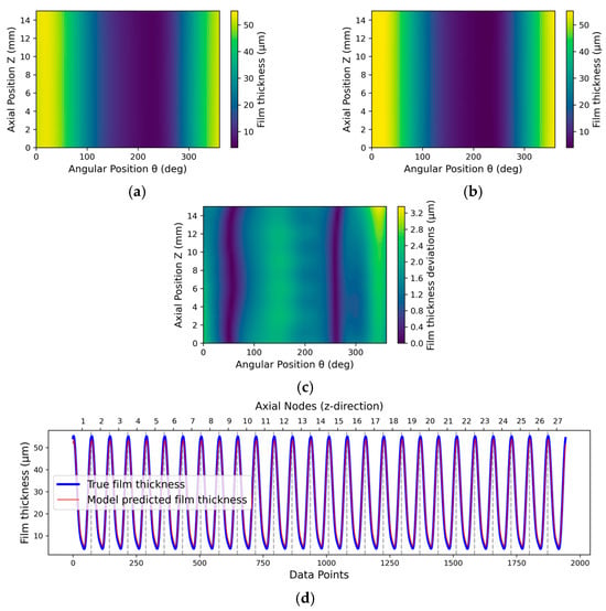
Figure 15.
Evaluation of the oil film thickness prediction for Case 2 (outside testing): (a) predicted values, (b) true values, (c) 2D deviation between true and predicted values, (d) 1D comparison between true and predicted values.
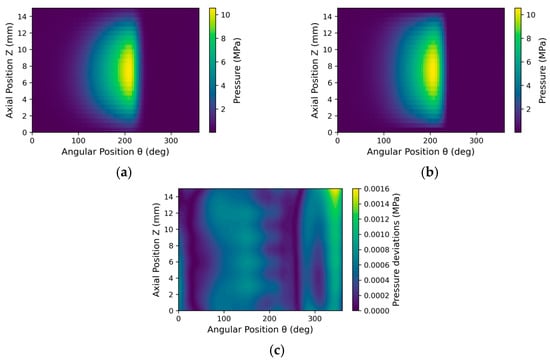

Figure 16.
Evaluation of the hydrodynamic pressure prediction for Case 7 (outside testing): (a) predicted values, (b) true values, (c) 2D deviation between true and predicted values, (d) 1D comparison between true and predicted values.
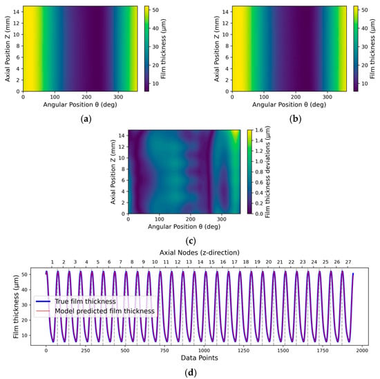
Figure 17.
Evaluation of the oil film thickness prediction for Case 7 (outside testing): (a) predicted values, (b) true values, (c) 2D deviation between true and predicted values, (d) 1D comparison between true and predicted values.
Remarkably, based on the results in Table 5, the model maintained reasonable predictive performance beyond the training domain, highlighting its robustness and generalisation capability. However, the accuracy was not as high as that observed within the training domain, particularly for peak pressure and minimum oil film thickness. This deviation is likely due to the scaling method and data processing used during training. As mentioned before (see Section 2.2.2), the inputs fed into the neural network component were normalised based on their maximum values. This scaling was applied only during the neural network block; therefore, when calculating the Reynolds equation residual or the load balancing constraints, the data were denormalised and relied on the same maximum values. After prediction, and before passing the results to the physics-based component, the outputs were rescaled. The model again relied on the same maximum values for this reverse normalisation. While this approach is straightforward, it can lead to deviations when the model encounters values outside the original scaling range.
In summary, these results confirm the effectiveness of the proposed PINN framework and its real-time model in predicting hydrodynamic pressure and oil film thickness, both inside and outside the trained domain. The results from both domains demonstrate the potential of this modelling method, showing that even with a limited number of cases, the model effectively captures a wide range of loads and speeds. This capability suggests that the model can generalise well across different operating conditions, providing valuable insights into hydrodynamic pressure and oil film thickness predictions. Nevertheless, several limitations should be addressed in future work to enhance the model’s realism and practical applicability. This includes refining the scaling method and data processing techniques. Additional limitations involve incorporating surface roughness effects, accounting for dynamic and transient loading conditions, and considering mixed lubrication regimes. This limitations of the proposed framework, along with the case study, allow for comparison with the analytical short-bearing approach under similar assumptions [20,21]. However, the proposed framework captures shaft and bearing flexibility through a 2D formulation that includes axial effects, overcoming the geometric simplifications of short-bearing theory. Even when evaluated outside its training or validity range, the PINN framework maintains errors within a reasonable margin, providing more robust and generalisable predictions compared to the short-bearing model when applied beyond its domain of validity. Moreover, the current PINN framework focuses on steady-state radial loading and does not yet account for mixed-friction effects. However, these limitations can be addressed in future work without compromising its real-time capabilities. This flexibility stands in contrast to traditional short-bearing models, which lack the adaptability for such extensions.
Furthermore, the enhanced efficiency of the PINN framework, combined with its flexibility, provides a solid foundation for real-time load monitoring in plain bearings. It allows for the direct incorporation of additional physical effects such as dynamic and transient loading conditions or mixed lubrication regimes. Future work can build on this to address both hydrodynamic and mixed-friction behaviour under transient loads.
4. Conclusions
This study presents an approach for load monitoring in radial plain bearings using PINNs. It extends the application of PINNs by relying solely on simple sensor inputs, such as radial load and rotational speed, to predict both the hydrodynamic pressure and oil film thickness distribution. This framework significantly expands the solution domain of PINNs, enabling generalisation across a wide range of steady-state operating conditions with varying loads and rotational speeds. This is achieved by enlarging the neural network structure and integrating additional physical constraints, such as load balancing, alongside the Reynolds equation.
The developed real-time model, based on the proposed framework, was evaluated within and beyond its training domain using results from 35 EHD simulation load cases. The reported percentage errors, approximately 1% and 2% within the training domain and around 5% and 12% outside, refer to the predicted peak hydrodynamic pressure and minimum oil film thickness, respectively. While these percentage errors may seem significant, the corresponding absolute errors are relatively small due to the narrow range of true values. The minimum oil film thickness, which has the highest error percentage and is critical for identifying unsafe operating conditions, is taken as an example here. Within the training domain, the minimum oil film thickness ranges from 4 to 10 μm, so a 2% error corresponds to an absolute deviation of about 0.1 to 0.2 μm. Outside the training domain, where values typically range from 3.7 to 10 μm, a 12% error results in a deviation of approximately 0.4 to 1.8 μm. On average across all cases, the absolute error remains below 0.5 μm, which can be considered low, while still leaving room for future improvements to further reduce deviation. The deviations occurring outside the training domain are likely due to the scaling method and data processing used during training, where the maximum and minimum values are known. However, these deviations are minimal, especially in the bearing’s loading zone, which highlights the model’s ability to generalise effectively across a wide range of loads and speeds. The developed model demonstrates efficiency by generating predictions in under one second for each test case, making it a practical tool for real-time load monitoring in plain bearings. While the model does not directly simulate failure mechanisms, its ability to predict key indicators such as minimum film thickness under various operating conditions makes it highly relevant for the early detection of lubrication risks and performance degradation.
Future work should consider the mixed-friction regime, including the incorporation of the lambda ratio. Additionally, accounting for dynamic loads would further improve the model’s applicability and extend its validity range. These enhancements would better reflect real-world applications such as marine propulsion systems, where reliable lubrication monitoring is essential to prevent costly failures.
Author Contributions
Conceptualisation, A.S.; Methodology, A.S.; Software, A.S.; Validation, A.S.; Formal analysis, A.S. and D.K.; Investigation, A.S. and D.K.; Resources, G.J.; Data curation, A.S.; Writing—original draft preparation, A.S.; Writing—review and editing, G.J., B.L. and M.L.; Visualisation, A.S.; Supervision, G.J. All authors have read and agreed to the published version of the manuscript.
Funding
This research received no external funding and the APC was funded by RWTH Aachen.
Data Availability Statement
The data presented in this study are available on request from the corresponding author.
Conflicts of Interest
The authors declare no conflicts of interest.
References
- Moder, J.; Bergmann, P.; Grün, F. Lubrication Regime Classification of Hydrodynamic Journal Bearings by Machine Learning Using Torque Data. Lubricants 2018, 6, 108. [Google Scholar] [CrossRef]
- Baszenski, T.; Kauth, K.; Kratz, K.-H.; Gutiérrez Guzmán, F.; Jacobs, G.; Gemmeke, T. Sensor integrating plain bearings: Design of an energy-autonomous, temperature-based condition monitoring system. Forsch. Im Ingenieurwesen 2023, 87, 441–452. [Google Scholar] [CrossRef]
- Gilges, M.; Saleh, A.; Bekker, A.; Jain, M.; Lehmann, B.; Jacobs, G. Influence of Propeller–Ice Loads on the Wear Development in Stern Tube Bearings of Marine Propulsion Systems and Identification of Critical Operating Conditions. J. Offshore Mech. Arct. Eng. 2024, 146, 061602. [Google Scholar] [CrossRef]
- Saleh, A.; Könekamp, M.; Jacobs, G.; Gilges, M.; Lehmann, B.; Lucassen, M. Evaluation of fatigue damage in stern tube sliding bearings of ship propulsion systems under ice impact. Forsch. Im Ingenieurwesen 2025, 89, 32. [Google Scholar] [CrossRef]
- Lucassen, M.; Jacobs, G.; Lehmann, B. Efficient dynamic simulations of planetary journal bearings in wind turbine gearboxes. Forsch. Im Ingenieurwesen 2025, 89, 20. [Google Scholar] [CrossRef]
- König, F.; Ouald Chaib, A.; Jacobs, G.; Sous, C. A multiscale-approach for wear prediction in journal bearing systems—From wearing-in towards steady-state wear. Wear 2019, 426, 1203–1211. [Google Scholar] [CrossRef]
- Sander, D.E.; Allmaier, H. Starting and stopping behavior of worn journal bearings. Tribol. Int. 2018, 127, 478–488. [Google Scholar] [CrossRef]
- Koetz, F.; Schmitt, F.; Kirchner, E.; Zancul, E. Visualising the lubrication condition in hydrodynamic journal bearings using impedance measurement. Front. Mech. Eng. 2024, 10, 1456575. [Google Scholar] [CrossRef]
- Xu, F.; Ding, N.; Li, N.; Liu, L.; Hou, N.; Xu, N.; Guo, W.; Tian, L.; Xu, H.; Lawrence Wu, C.-M.; et al. A review of bearing failure Modes, mechanisms and causes. Eng. Fail. Anal. 2023, 152, 107518. [Google Scholar] [CrossRef]
- Scott, K.; Infield, D.; Barltrop, N.; Coultate, J.; Shahaj, A. Effects of Extreme and Transient Loads on Wind Turbine Drive Trains. In Proceedings of the 50th AIAA Aerospace Sciences Meeting including the New Horizons Forum and Aerospace Exposition, Nashville, TN, USA, 9–12 January 2012; American Institute of Aeronautics and Astronautics: Reston, VA, USA, 2012; p. 01092012, ISBN 978-1-60086-936-5. [Google Scholar]
- Abadi, N.M.M. Überwachung Hydrodynamischer Gleitlager Basierend auf der Körperschallanalyse. Master’s Dissertation, Technische Universität Berlin, Berlin, Germany, 2020. [Google Scholar]
- Brinkschulte, L.; Geimer, M. Real-time Estimation of the Remaining Lifetime of Components. ATZoffhighway Worldw. 2017, 10, 54–60. [Google Scholar] [CrossRef]
- Pagitsch, M.; Jacobs, G.; Bosse, D. Remaining Useful Life Determination for Wind Turbines. J. Phys. Conf. Ser. 2020, 1452, 12052. [Google Scholar] [CrossRef]
- Wright, L.; Davidson, S. How to tell the difference between a model and a digital twin. Adv. Model. Simul. Eng. Sci. 2020, 7, 13. [Google Scholar] [CrossRef]
- Reynolds, O. IV. On the theory of lubrication and its application to Mr. Beauchamp tower’s experiments, including an experimental determination of the viscosity of olive oil. Philos. Trans. R. Soc. 1886, 177, 157–234. [Google Scholar] [CrossRef]
- AVL-List GmbH. EXCITE Power Unit User Manual (R2022.1); AVL-List GmbH: Graz, Austria, 2022. [Google Scholar]
- Cartwright, S.; Rothwell, B.C.; Figueredo, G.; Medina, H.; Eastwick, C.; Layton, J.; Ambrose, S. A machine learning-driven approach to predicting thermo-elasto-hydrodynamic lubrication in journal bearings. Tribol. Int. 2024, 196, 109670. [Google Scholar] [CrossRef]
- DIN 31652-1:2017-01; Gleitlager Hydrodynamische Radial-Gleitlager im stationären Betrieb—Teil 1: Berechnung von Kreiszylinderlagern. DIN Media, GmbH: Berlin, Germany, 2017.
- Vogelpohl, G. (Ed.) Beiträge zur Gleitlagerberechnung; Forschungsheft nr. 386; VDI: Düsseldorf, Germany, 1954. [Google Scholar]
- Kirk, R.G.; Gunter, E.J. Short Bearing Analysis Applied to Rotor Dynamics—Part I: Theory. J. Lubr. Technol. 1976, 98, 47–56. [Google Scholar] [CrossRef]
- DuBois, G.B.; Ocvirk, F.W. The Short Bearing Approximation for Plain Journal Bearings. J. Fluids Eng. 1955, 77, 1173–1178. [Google Scholar] [CrossRef]
- Faria, M.T.C. On the Hydrodynamic Long Journal Bearing Theory. In Proceedings of the World Congress on Engineering 2014, WCE 2014, London, UK, 2–4 July 2014; Volume II, ISBN 978-988-19253-5-0, ISSN 2078-0958 (Print)/2078-0966 (Online). [Google Scholar]
- Timbó, R.; Martins, R.; Bachmann, G.; Rangel, F.; Mota, J.; Valério, J.; Ritto, T. ROSS-Rotordynamic Open Source Software. J. Open Source Softw. 2020, 5, 2120. [Google Scholar] [CrossRef]
- Marian, M.; Bartz, M.; Wartzack, S.; Rosenkranz, A. Non-Dimensional Groups, Film Thickness Equations and Correction Factors for Elastohydrodynamic Lubrication: A Review. Lubricants 2020, 8, 95. [Google Scholar] [CrossRef]
- Daniel, C. Simulation von gleit- und wälzgelagerten Systemen auf Basis eines Mehrkörpersystems für rotordynamische Anwendungen. Doctoral Dissertation, Otto-von-Guericke-Universität, Magdeburg, Germany, 2013. [Google Scholar]
- Gong, R.-Z.; Li, D.-Y.; Wang, H.-J.; Han, L.; Qin, D.-Q. Analytical solution of Reynolds equation under dynamic conditions. Proc. Inst. Mech. Eng. Part J J. Eng. Tribol. 2016, 230, 416–427. [Google Scholar] [CrossRef]
- Mauro, F.; Kana, A.A. Digital twin for ship life-cycle: A critical systematic review. Ocean. Eng. 2023, 269, 113479. [Google Scholar] [CrossRef]
- Marian, M.; Tremmel, S. Current Trends and Applications of Machine Learning in Tribology—A Review. Lubricants 2021, 9, 86. [Google Scholar] [CrossRef]
- Marian, M.; Tremmel, S. Physics-Informed Machine Learning—An Emerging Trend in Tribology. Lubricants 2023, 11, 463. [Google Scholar] [CrossRef]
- Rosenkranz, A.; Marian, M.; Profito, F.J.; Aragon, N.; Shah, R. The Use of Artificial Intelligence in Tribology—A Perspective. Lubricants 2021, 9, 2. [Google Scholar] [CrossRef]
- Sadık Ünlü, B.; Durmuş, H.; Meriç, C. Determination of tribological properties at CuSn10 alloy journal bearings by experimental and means of artificial neural networks method. Ind. Lubr. Tribol. 2012, 64, 258–264. [Google Scholar] [CrossRef]
- Hess, N.; Shang, L. Development of a Machine Learning Model for Elastohydrodynamic Pressure Prediction in Journal Bearings. J. Tribol. 2022, 144, 081603. [Google Scholar] [CrossRef]
- Raissi, M.; Perdikaris, P.; Karniadakis, G.E. Physics Informed Deep Learning (Part I): Data-driven Solutions of Nonlinear Partial Differential Equations. arXiv 2017, arXiv:1711.10561. [Google Scholar] [CrossRef]
- Raissi, M.; Perdikaris, P.; Karniadakis, G.E. Physics Informed Deep Learning (Part II): Data-driven Discovery of Nonlinear Partial Differential Equations. arXiv 2017, arXiv:1711.10566. [Google Scholar] [CrossRef]
- Raissi, M.; Perdikaris, P.; Karniadakis, G.E. Physics-informed neural networks: A deep learning framework for solving forward and inverse problems involving nonlinear partial differential equations. J. Comput. Phys. 2019, 378, 686–707. [Google Scholar] [CrossRef]
- Rom, M. Physics-informed neural networks for the Reynolds equation with cavitation modeling. Tribol. Int. 2023, 179, 108141. [Google Scholar] [CrossRef]
- Markidis, S. The Old and the New: Can Physics-Informed Deep-Learning Replace Traditional Linear Solvers? Front. Big Data 2021, 4, 669097. [Google Scholar] [CrossRef]
- Almqvist, A. Fundamentals of Physics-Informed Neural Networks Applied to Solve the Reynolds Boundary Value Problem. Lubricants 2021, 9, 82. [Google Scholar] [CrossRef]
- Zhao, Y.; Guo, L.; Wong, P.P.L. Application of physics-informed neural network in the analysis of hydrodynamic lubrication. Friction 2023, 11, 1253–1264. [Google Scholar] [CrossRef]
- Li, L.; Li, Y.; Du, Q.; Liu, T.; Xie, Y. ReF-nets: Physics-informed neural network for Reynolds equation of gas bearing. Comput. Methods Appl. Mech. Eng. 2022, 391, 114524. [Google Scholar] [CrossRef]
- Cheng, Y.; He, Q.; Huang, W.; Liu, Y.; Li, Y.; Li, D. HL-nets: Physics-informed neural networks for hydrodynamic lubrication with cavitation. Tribol. Int. 2023, 188, 108871. [Google Scholar] [CrossRef]
- Xi, Y.; Deng, J.; Li, Y. A solution for finite journal bearings by using physics-informed neural networks with both soft and hard constrains. Ind. Lubr. Tribol. 2023, 75, 560–567. [Google Scholar] [CrossRef]
- Shutin, D.; Kazakov, Y.; Stebakov, I.; Savin, L. Data-driven and physics-informed approaches for improving the performance of dynamic models of fluid film bearings. Tribol. Int. 2024, 191, 109136. [Google Scholar] [CrossRef]
- Zhou, G.; Zhan, M.; Huang, D.; Lyu, X.; Yan, K. Enhanced PINNs with augmented Lagrangian method and transfer learning for hydrodynamic lubrication analysis. Ind. Lubr. Tribol. 2024, 76, 1246–1255. [Google Scholar] [CrossRef]
- Ramos, D.J.; Cunha, B.Z.; Daniel, G.B. Evaluation of physics-informed neural networks (PINN) in the solution of the Reynolds equation. J. Braz. Soc. Mech. Sci. Eng. 2023, 45, 568. [Google Scholar] [CrossRef]
- Brumand-Poor, F.; Bauer, N.; Plückhahn, N.; Thebelt, M.; Woyda, S.; Schmitz, K. Extrapolation of Hydrodynamic Pressure in Lubricated Contacts: A Novel Multi-Case Physics-Informed Neural Network Framework. Lubricants 2024, 12, 122. [Google Scholar] [CrossRef]
- Purcell, E.; Nejad, A.R.; Böhm, A.; Sapp, L.; Lund, J.; von Bock und Polach, F.; Nickerson, B.M.; Bekker, A.; Gilges, M.; Saleh, A.; et al. On Methodology for a Digital Twin of Ship Propulsion Under Harsh Environmental Conditions. In Volume 6: Polar and Arctic Sciences and Technology; CFD, FSI, and AI, Proceedings of ASME 2024 43rd International Conference on Ocean, Offshore and Arctic Engineering, Singapore, 9–14 June 2024; American Society of Mechanical Engineers: Little Falls, NJ, USA, 2024; p. 06092024. ISBN 978-0-7918-8784-4. [Google Scholar]
- Moseley, B.; Markham, A.; Nissen-Meyer, T. Finite basis physics-informed neural networks (FBPINNs): A scalable domain decomposition approach for solving differential equations. Adv. Comput. Math. 2023, 49, 62. [Google Scholar] [CrossRef]
- Allmaier, H.; Offner, G. Current Challenges and Frontiers for the EHD Simulation of Journal Bearings: A Review; SAE Technical Paper 2016-01-1856; SAE: Warrendale, PA, USA, 2016. [Google Scholar]
- Schmidt, J.H. An Efficient Solution Procedure for Elastohydrodynamic Contact Problems Considering Structural Dynamics; KIT Scientific Publishing: Karlsruhe, Germany, 2019; Volume 33. [Google Scholar]
- Nikolakopoulos, P.G.; Papadopoulos, C.A. Non-linearities in misaligned journal bearings. Tribol. Int. 1994, 27, 243–257. [Google Scholar] [CrossRef]
- Wei, W.; Guo, W.; Han, J.; Wu, X. A new method calculating load balance of sliding bearing by using neural network PID algorithm. Vibroeng. Procedia 2018, 21, 225–230. [Google Scholar] [CrossRef]
- König, F.; Sous, C.; Jacobs, G. Numerical prediction of the frictional losses in sliding bearings during start-stop operation. Friction 2021, 9, 583–597. [Google Scholar] [CrossRef]
- König, F.; Wirsing, F.; Singh, A.; Jacobs, G. Machine-Learning-Based Wear Prediction in Journal Bearings under Start–Stop Conditions. Lubricants 2024, 12, 290. [Google Scholar] [CrossRef]
- Greenwood, J.A.; Tripp, J.H. The Contact of Two Nominally Flat Rough Surfaces. Proc. Inst. Mech. Eng. 1970, 185, 625–633. [Google Scholar] [CrossRef]
- Patir, N.; Cheng, H.S. An Average Flow Model for Determining Effects of Three-Dimensional Roughness on Partial Hydrodynamic Lubrication. J. Lubr. Technol. 1978, 100, 12–17. [Google Scholar] [CrossRef]
- Chen, Y.; Koohy, S. GPT-PINN: Generative Pre-Trained Physics-Informed Neural Networks toward non-intrusive Meta-learning of parametric PDEs. arXiv 2023, arXiv:2303.14878. [Google Scholar] [CrossRef]
- Hosseini Dashtbayaz, N.; Farhani, G.; Wang, B.; Ling, C.X. Physics-Informed Neural Networks: Minimizing Residual Loss with Wide Networks and Effective Activations. arXiv 2024, arXiv:2405.01680. [Google Scholar] [CrossRef]
- Baydin, A.G.; Pearlmutter, B.A.; Radul, A.A.; Siskind, J.M. Automatic differentiation in machine learning: A survey. arXiv 2015, arXiv:1502.05767. [Google Scholar] [CrossRef]
- He, K.; Zhang, X.; Ren, S.; Sun, J. Delving Deep into Rectifiers: Surpassing Human-Level Performance on ImageNet Classification. In Proceedings of the IEEE international conference on computer vision, Santiago, Chile, 7–13 December 2015; pp. 1026–1034. [Google Scholar]
- Toscano, J.D.; Oommen, V.; Varghese, A.J.; Zou, Z.; Daryakenari, N.A.; Wu, C.; Karniadakis, G.E. From PINNs to PIKANs: Recent Advances in Physics-Informed Machine Learning. arXiv 2024, arXiv:2410.13228. [Google Scholar] [CrossRef]
- Xiang, Z.; Peng, W.; Liu, X.; Yao, W. Self-adaptive loss balanced Physics-informed neural networks. Neurocomputing 2022, 496, 11–34. [Google Scholar] [CrossRef]
- Song, C.; Kawai, R. Monte Carlo and variance reduction methods for structural reliability analysis: A comprehensive review. Probabilistic Eng. Mech. 2023, 73, 103479. [Google Scholar] [CrossRef]
Disclaimer/Publisher’s Note: The statements, opinions and data contained in all publications are solely those of the individual author(s) and contributor(s) and not of MDPI and/or the editor(s). MDPI and/or the editor(s) disclaim responsibility for any injury to people or property resulting from any ideas, methods, instructions or products referred to in the content. |
© 2025 by the authors. Licensee MDPI, Basel, Switzerland. This article is an open access article distributed under the terms and conditions of the Creative Commons Attribution (CC BY) license (https://creativecommons.org/licenses/by/4.0/).

