Article

Rolling Bearing Fault Diagnosis across Operating Conditions Based on Unsupervised Domain Adaptation

1
College of Mechanical and Electrical Engineering, Henan University of Science and Technology, Luoyang 471023, China
2
School of Computer and Information Engineering, Henan Normal University, Xinxiang 453007, China
3
State Key Laboratory of Aerospace Precision Bearings, Luoyang 471000, China
*
Author to whom correspondence should be addressed.
Lubricants 2023, 11(9), 383; https://doi.org/10.3390/lubricants11090383
Submission received: 3 August 2023 / Revised: 26 August 2023 / Accepted: 1 September 2023 / Published: 8 September 2023
(This article belongs to the Special Issue Recent Advances in Machine Learning in Tribology)

Abstract

:
In practical industrial scenarios, mechanical equipment frequently operates within dynamic working conditions. To address the challenge posed by the incongruent data distribution between source and target domains amidst varying operational contexts, particularly in the absence of labels within the target domain, this study presents a solution involving deep feature construction and an unsupervised domain adaptation strategy for rolling bearing fault diagnosis across varying working conditions. The proposed methodology commences by subjecting the original vibration signal of the bearing to a fast Fourier transform (FFT) to extract spectral information. Subsequently, an innovative amalgamation of a one-dimensional convolutional layer and an auto-encoder were introduced to construct a convolutional auto-encoder (CAE) dedicated to acquiring depth features from the spectrum. In a subsequent step, leveraging the depth features gleaned from the convolutional auto-encoder, a balanced distribution adaptation (BDA) mechanism was introduced to facilitate the domain adaptation of features from both the source and target domains. The culminating stage entails the classification of adapted features using the K-nearest neighbor (KNN) algorithm to attain cross-domain diagnosis. Empirical evaluations are conducted on two extensively used datasets. The findings substantiate that the proposed approach is capable of accomplishing the cross-domain fault diagnosis task even without labeled data within the target domain. Furthermore, the diagnostic accuracy and stability of the proposed method surpass those of various other migration and deep learning approaches.

1. Introduction

Rolling bearings stand as vital constituents within rotating machinery and equipment, with extensive applications in domains such as wind power generation, aerospace, and numerous others [1,2]. Due to their regular exposure to elevated temperatures, heavy loads, dynamic operational conditions, and other demanding and intricate work settings, the reliability of rolling bearings is subject to diminishment. A single instance of failure can engender disruptions in regular industrial production and potentially yield considerable economic repercussions, in some cases, even posing a threat to human life [3]. As indicated in references [4,5,6], bearing failures contribute to 45–90% of the overall error occurrences in certain machinery and equipment. Thus, undertaking research on intelligent fault diagnosis specifically targeting rolling bearings [7] is of paramount importance.
The vibration signal encapsulates a wealth of information pertaining to the bearing’s health condition, forming the foundation for the majority of ongoing research [8]. As stipulated by the literature [9], fault diagnosis techniques can be broadly categorized into two groups: model-based approaches and data-driven methods. Model-based fault diagnosis methodologies often entail the construction of physical models for characterizing bearing defects [10,11]. Nonetheless, this method heavily relies on a priori knowledge of industrial systems and associated components. The actual operation of industrial systems is marked by uncertainties linked to operational conditions, noise, and other factors, and the assumptions underpinning the model fail to accommodate these sources of uncertainty.
Data-driven methodologies commonly leverage techniques encompassing signal processing, statistical feature extraction, and machine learning for fault diagnosis. Singh introduces a fault diagnosis approach grounded in wavelet analysis [12]. Meanwhile, Wang et al. put forth a nonlinear time-frequency flow form learning technique tailored for bearing fault diagnosis [13], its efficacy being substantiated through application to actual bearings. Shazali Osman et al. introduced a novel morphological Hilbert Huang (MH) approach aimed at the early detection of bearing failures [14]. Empirical mode decomposition (EMD) stands as a classical signal processing technique widely applied in the realm of bearing fault diagnosis [15]. Complementing this, variational mode decomposition (VMD) presents a more sophisticated signal-adaptive decomposition methodology [16]. Wang et al. [17] employ VMD in conjunction with cyclic correlation entropy functions for bearing fault diagnosis. Nevertheless, the aforementioned techniques often necessitate the involvement of domain experts during the diagnosis process, a practice prone to intricacies in computation. In related investigations, signal processing serves as the basis for feature extraction, frequently entailing the manual extraction of pertinent attributes encompassing time and frequency domains, as well as signal entropy [18]. Zhang et al. [19] conducted feature extraction from bearing vibration signals, yielding six time and thirteen frequency-domain features tailored for fault diagnosis. Entropy stands as a quantitative tool to delineate the system complexity and has found utility within the domain of vibration signal analysis [20]. Li et al. introduced multiscale dispersion entropy (MDE) for scrutinizing bearing vibration signals and effecting feature extraction [21]. Jiao et al. merged multi-scale sample entropy (MSE) with Energy Moment (EM) for extracting bearing features [22]. Despite attaining a certain degree of accuracy and stability, these methods can only partially accomplish bearing fault diagnosis. Nonetheless, the manual extraction of fault-related features remains an intricate endeavor. This accentuates the pivotal importance of research in automating feature extraction and ensuring the fluid implementation of end-to-end fault diagnosis.
The advancement of artificial intelligence has garnered scholarly attention toward machine learning technology. This genre of technology undertakes data processing to unearth data patterns [23]. Malhi et al. harnessed the principal component analysis (PCA) algorithm to derive bearing signal features, subsequently feeding these features into radial basis function (RBF) networks for fault classification [24]. The support vector machine (SVM) stands as a classical machine learning classifier. Yang et al. utilized intrinsic mode functions (IMF) such as SVM input vectors, with the output indicating bearing failure modes [25]. Pandya et al. accomplished bearing fault diagnosis by relying on acoustic emission signals and a K-nearest neighbor (KNN) classifier. In addition, algorithms such as singular value decomposition (SVD) [26] and the Naive Bayes classifier [27] have also achieved success in bearing fault diagnosis. Notably, while these machine learning-oriented methods operate without human intervention, they are characterized as shallow, possessing limited learning capacities. Moreover, they often struggle to extract high-quality features from intricate, non-linear, and high-dimensional data [22].
Recent years have witnessed the proliferation of deep learning in the realm of fault diagnosis, with deep neural networks displaying formidable prowess in feature extraction [28]. Xia et al. introduced a multi-sensor fusion approach grounded in a convolutional neural network (CNN), proficiently engendering adaptively extracted signal features conducive to end-to-end fault diagnosis [29]. Shao et al. crafted a deep belief network (DBN) to autonomously capture representative features inherent to the original feature set [30]. Sun et al. harnessed a sparse auto-encoder (SAE) to master the features within vibration signals, followed by classification of the extracted features for fault analysis via a deep neural network (DNN) [31]. Kerboua et al. [32] devised a fresh technique for asynchronous motor fault diagnosis, capitalizing on three-dimensional convolutional neural networks. This innovation wields the potential to significantly curtail downtime and optimize production efficiency. Liang et al. [33] formulated a novel approach for diagnosing rolling bearing faults by leveraging the ICEEMDAN Hilbert and ResNet. This method adeptly tackles issues of neutral energy degradation and pivotal feature information loss within deep learning networks.
Deep learning methods possess the capability to autonomously extract fault features, yielding features that effectively capture the essence of the original signal. Nevertheless, the implementation of deep learning methods relies on two key assumptions: (1) the network training data necessitates supervised learning, entailing a substantial volume of labeled data; and (2) both the training and testing data in the source and target domains adhere to an identical distribution. It is crucial to recognize that these two presumptions frequently fall short in real-world scenarios owing to shifts in operational contexts, environmental interference, and assorted external factors. Procuring substantial quantities of labeled data proves highly costly, and data distribution often fluctuates in accordance with working conditions, collectively constraining the advantages of deep learning algorithms. Domain adaptation (DA) emerges as a potent strategy for mitigating the dearth of labeled data and ameliorating imbalanced data distribution, thereby redressing the inherent limitations of deep learning [34,35]. Wei et al. employed transfer component analysis (TCA) to transfer the vibration characteristics of bearings under various operating conditions [36]. Lu et al. utilized maximum mean discrepancy (MMD) for measuring feature distribution deviation across distinct domains, thereby minimizing the gap between the source and target domains [37]. Li et al. amalgamated joint distribution adaptation (JDA) with SVM, employing JDA to assess both the boundary and conditional distributions of data features, while employing SVM as a fault classifier [38]. However, TCA and MMD, for instance, solely focus on the edge distribution of the data. While JDA is capable of adapting both edge and conditional distributions, it neglects the joint contribution of these distributions during adaptation. Balanced distribution adaptation (BDA), proposed by Wang et al., introduces a balancing factor to JDA, enabling dynamic adjustment of the significance of both edge and conditional distributions [39].
In this study, we synergize deep learning and domain adaptation strategies to introduce a novel model for bearing fault diagnosis that relies on both deep learning and unsupervised domain adaptation principles. This model autonomously captures data features, mitigates the challenge of insufficiently labeled data, and aligns data distributions across domains. Initially, an unsupervised convolutional auto-encoder is established for adaptive data feature extraction across both source and target domains. Subsequently, the introduction of balanced distribution adaptation (BDA) serves to minimize the separation between data in the source and target domains. Ultimately, the K-nearest neighbor (KNN) algorithm, trained on the source domain, is employed for the classification of data in the target domain. The primary contributions of this study are summarized below:
(1) We propose a framework that leverages deep learning and unsupervised domain adaptation to address variable working condition problems. This framework autonomously extracts features from raw data, harnesses the advantages of both deep learning and domain adaptation, and facilitates fault diagnosis;
(2) We introduce the BDA algorithm to handle the feature distance metric and migration. This facilitates domain adaptation by balancing the edge distribution and conditional distribution of the data;
(3) We employ TSNE technology to visualize every stage of feature extraction and migration. This approach elucidates the detailed patterns of data transformation and offers interpretability for both the migration and deep learning algorithms.

2. Theoretical Foundation

2.1. Fast Fourier Transform (FFT)

FFT [40] represents an engineered realization of the discrete Fourier transform (DFT), streamlining the computational procedure. Employing the FFT transformation in the time-domain vibration signal of the bearing facilitates the acquisition of frequency domain particulars. Unique fault patterns are encapsulated within distinct frequency bands, rendering the frequency domain signal more adept for fault diagnosis compared to the original vibration signal [41]. Zhang et al. conducted an FFT transformation on vibration signals and derived features from the resultant spectral signals to facilitate bearing fault diagnosis [42]. On the other hand, Mao et al. applied an FFT transformation to the bearing vibration signal, and the ensuing spectral information underwent processing via a generative adversarial network (GAN) [43], which was employed for the early detection of bearing failures.
For a finite length bearing time-domain vibration discrete signal x ( n ) , the spectral function X ( k ) can be obtained via DFT:
X ( k ) = n = 0 N 1 x ( n ) ω N k n , 0 k N 1
where, N is the sample length, ω N = e j 2 π N .
FFT decomposes the sequence x ( n ) into two parts, an even sequence x 2 ( n ) and an odd sequence x 1 ( n ) , each with the length N 2 . Thus, we obtain
X ( k ) = n = 0 N 2 1 x 1 ( n ) ω N 2 k n + n = 0 N 2 x 2 ( n ) ω N ( 2 k + 1 ) n
Extracting the factorization of Equation (2) yields
X ( k ) = n = 0 N 2 1 x 1 ( n ) ω N 2 k n + ω N k n n = 0 N 2 x 2 ( n ) ω N 2 k n
Since ω N 2 k = e j 2 π N 2 k n = e j 2 π N / 2 k n = ω N / 2 k n , integrating it into Equation (3) yields
X ( k ) = n = 0 N 2 1 x 1 ( n ) ω N / 2 k n + ω N k n n = 0 N 2 1 x 2 ( n ) ω N / 2 k n = X 1 ( k ) + ω N k X 2 ( k )
where, X 1 ( k ) is the result of the odd sequence x 1 ( n ) and X 2 ( k ) is the result of the even sequence x 2 ( n ) .

2.2. Autoencoder (AE)

AE [44], an established unsupervised learning algorithm, undertakes the task of reconstructing input data into outputs. The utilization of AE and its adaptations has found extensive application within the realm of bearing analysis. Mao et al. employed a stacked denoising auto-encoder to extract shared features among various health states of bearings [45]. Similarly, Jing et al. employed AE to capture spectral features from the signal and coupled it with a Gaussian mixture model for clustering [46]. A representative self-coding structure is illustrated in Figure 1.
AE typically comprises two components: an encoder and a decoder. The encoder is capable of reducing the dimensionality of the input signal and extracting features, while the decoder reconstructs the input signal by employing the extracted features as the input.
If the input to the encoder is assumed, and the resulting feature vector is obtained through encoding, then
h = f ( ω X + b )
where, f is the activation function, ω is the weight of the network, and b is the network bias.
In the decoding stage, the input of the decoder is h and the output is X ^ :
X ^ = f ( ω h + b )
where, f is the activation function, ω is the weight of the network, and b is the network bias.
The auto-encoder network updates the internal parameters by minimizing the reconfiguration error, where l A E is
l A E = | X X ^ | 2

2.3. Convolutional Neural Network (CNN)

CNN [47], a significant component in modern deep learning, is distinguished by its attributes of parameter sharing and translation invariance. These attributes facilitate the extraction of robust features and have contributed to its widespread use in the context of diagnosing faults in rolling bearings [48]. The structure of a one-dimensional convolutional network primarily comprises a one-dimensional convolutional layer, a one-dimensional pooling layer, a fully connected layer, and a classifier, as illustrated in Figure 2.
The convolution layer is composed of a convolutional kernel that executes convolution operations on the input signal and employs a nonlinear activation function to construct features. The resulting output is
y i l = j = 1 N x j l k j i l + b i l
where, y i l represents the jth convolutional computed vector of the lth layer, N is the number of input feature vectors, x j l is the jth input feature vector of the lth layer, represents the convolutional computation, k j i l is the convolutional kernel of the lth layer with the jth input feature vector, and b i l is the ith bias vector of the lth layer.
The output features typically undergo transformation through a nonlinear activation function subsequent to the convolution operation. In this study, the rectified linear unit (ReLU) was employed as the activation function. ReLU is formally defined as
a i l ( j ) = f ( y i l ( j ) ) = max ( 0 , y i l ( j ) ) = { y i l ( j ) y i l ( j ) 0 0 y i l ( j ) < 0
where, y i l ( j ) is the jth output after the ith convolution operation of the lth layer and a i l ( j ) is the activation value of y i l ( j ) .
Following ReLU activation, the feature vector is commonly subjected to dimensionality reduction through the utilization of a maximum pooling layer. This operation is computed as
p i l + 1 ( j ) = max ( j 1 ) w + 1 t j w { a i l ( t ) }
The fully connected layer can expand the output of the pooling layer to form a one-dimensional feature vector with the activation function ReLU; the softmax classification layer can perform the final multiclassification operation, assuming that the label is y { 1 , 2 , , K } , and given sample x, its probability of belonging to category k is
p ( y = k | x ; Θ ) = s o f t max ( θ k T x ) = exp ( θ k T x ) i = 1 K exp ( θ i T x )
where Θ is all the training parameters in the softmax regression model and 1 / i = 1 K exp ( θ i T x ) is the normalization function.

2.4. Balanced Distribution Adaptation (BDA)

A labeled source domain space was set as D S = { x s i , y s i } i = 1 n , and an unlabeled target domain space D t = { x t j } j = 1 n . The same feature space was assumed, but the different edge and conditional distributions were p ( x s ) p ( x t ) and p ( y s | x s ) p ( y t | x t ) .
BDA is a domain adaptive method that adaptively weighs the importance of the edge distribution and conditional distribution between domains by introducing a balancing factor, μ , that minimizes the following distances.
D ( D S , D t ) ( 1 μ ) ( P ( x s ) , P ( x t ) ) + μ ( P ( y s | x s ) , P ( y t | x t ) )
where, μ [ 0 , 1 ] is a balance factor measuring the importance of the edge distribution and the conditional distribution. When μ is close to 0, the edge distribution is given priority, and when it is close to 1, the conditional distribution is given priority.
It is important to note that since the target domain does not have sample labels, it is not possible to calculate the conditional distribution p ( y t | x t ) . Here, the class conditional distribution p ( x t | y t ) is used instead of p ( y t | x t ) . The classifier is trained in the target domain and used to predict the pseudo label in the target domain, thus calculating p ( x t | y t ) . This process is continuously iterated to improve reliability [46]. The difference between the two distributions was estimated using the maximum mean discrepancy (MMD) Equation (12), which was reduced to
D ( D S , D t ) ( 1 μ ) 1 n i = 1 n x s i 1 m j = 1 m x t j κ 2 + μ c = 1 C 1 n c x s i D s ( c ) x s i 1 m c x t j D t ( c ) x t j κ 2
where κ is the regenerative kernel Hilbert space, n is the number of samples in the source domain, m is the number of samples in the target domain, n c is the number of c-class samples in the source domain, and m c is the number of c-class samples in the target domain.
Continuing to use regularization and matrix transformation techniques, Equation (13) can be formalized as:
min t r ( A T X ( ( 1 μ ) M 0 + μ c = 1 C M c ) X T A ) + λ A F 2 s . t . A T X H X T A = I , 0 μ 1
where λ is the Frobenius coefficient of the regularization term · F 2 , X is the matrix consisting of x s and x t , A denotes the transformation matrix, I is the unit matrix, and H is the central matrix, H = I − (1/n). M 0 and M c are MMD matrices with the following expressions:
( M 0 ) i j = { 1 n 2 , x i , x j D s 1 m 2 , x i , x j D t 1 m n , o t h e r w i s e
( M c ) i j = { 1 n c 2 , x i , x j D s ( c ) 1 m c 2 , x i , x j D t ( c ) 1 m c n c , { x i D s ( c ) , x j D t ( c ) x i D t ( c ) , x j D s ( c ) 0 , o t h e r w i s e
The Lagrangian operator ϕ = ( ϕ 1 , ϕ 2 , , ϕ d ) is introduced and the Lagrangian function of Equations (14) and (15) is obtained by associating the following equation:
min t r ( A T X ( ( 1 μ ) M 0 + μ c = 1 C M c ) X T A ) + λ A F 2 s . t . A T X H X T A = I , 0 μ 1
Optimization can be viewed as a generalized reformulation problem, such that L / A = 0 , which yields
( X ( ( 1 μ ) M 0 + μ c = 1 C M c ) X T + λ I ) A = X H X T A ϕ
The optimal mapping transformation matrix A is obtained by solving for it.

3. Proposed Architecture

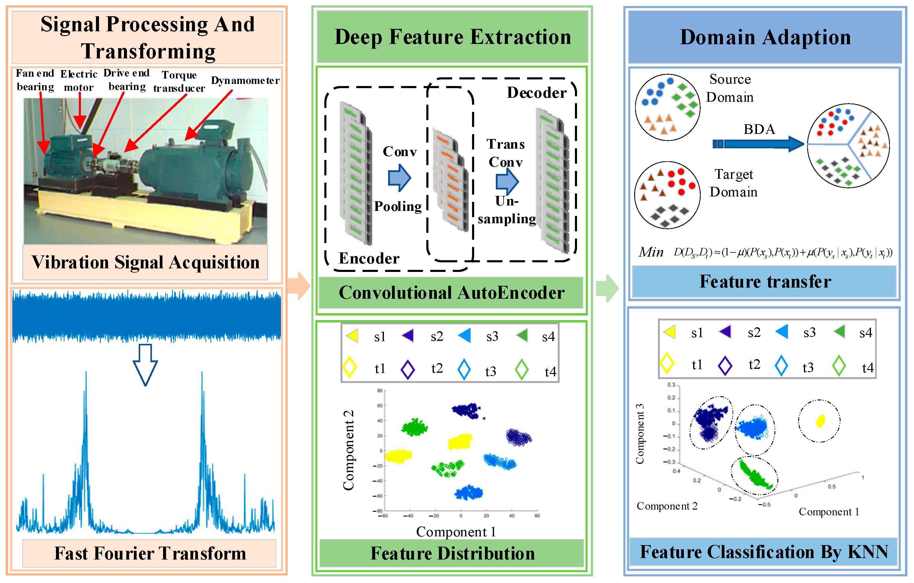
In order to enhance the precision of bearing fault diagnosis amidst varying operating conditions, this section introduces an unsupervised domain adaptive fault diagnosis framework that relies on autoencoder depth features and balanced distribution adaptation. The architectural layout of the network and core procedural steps are illustrated in Figure 3 and Figure 4. The detailed parameters governing the convolutional auto-encoder (CAE) network structure are provided in Table 1.
As depicted in Table 1, the initial convolutional layer extracts features directly from the input raw signal without undergoing additional transformations. The principal distinction between the comprehensive architecture of the devised CAE model and that of conventional CNN models resides at the filter level. Specifically, adopting a larger convolutional kernel in the inaugural layer is more adept at attenuating high-frequency noise, while the subsequent convolutional kernels are comparatively diminutive. The incorporation of multiple layers with smaller convolutional kernels enhances the network’s depth, consequently facilitating the acquisition of a robust representation of the input signal and expediting the training procedure.
The process is primarily divided into three sequential steps. First, the data undergo a fast Fourier transform to acquire spectral information. Subsequently, convolutional autoencoders are employed to extract depth features from the spectra. Lastly, the BDA algorithm is applied to facilitate domain adaptation. The specific procedures are elucidated as follows:
Step 1: Signal acquisition and preprocessing. Utilize acceleration sensors to capture raw vibration signals from rolling bearings under different operational conditions and fault types. Then, preprocess the signal by selecting 1024 original vibration data points as samples. Apply the fast Fourier transform to obtain the bilateral spectrum, and subsequently, perform z-score standardization on the spectrum.
Step 2: Deep feature extraction and migration. Construct a convolutional autoencoder model and employ FFT spectra as inputs for unsupervised deep feature extraction. Throughout the migration procedure, the encoder architecture of the convolutional autoencoder is capable of generating profound features. The BDA algorithm is then applied to modify the edge and condition distributions of features from the source and target domains, thereby achieving feature migration.
Step 3: Fault classification. The migrated features are shared, and the classification task employs the K-nearest neighbors (KNN) classifier.

4. Experiments and Analysis

In order to showcase the efficacy of the proposed approach, this section opts for the utilization of two extensively employed publicly accessible datasets for conducting cross-service fault diagnosis experiments (CWRU and SEU datasets).

4.1. Variable Load Dataset from the CWRU

4.1.1. Data Description

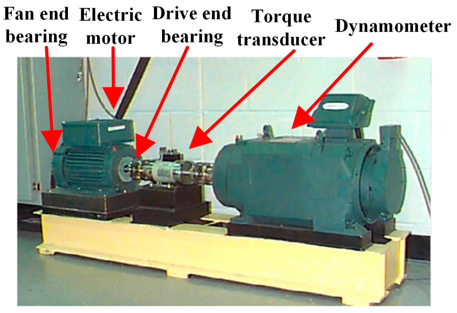
The CWRU bearing dataset was sourced from the Electrical Engineering Laboratory at the Case Western Reserve University, with the experimental setup as depicted in Figure 5.
Single-point damage was inflicted on the bearing arrangement using EDM, resulting in failure diameters of 0.007, 0.014, 0.021, and 0.028 inches, along with distinct failure types: outer ring failure, inner ring failure, and rolling element failure. Vibration data of the bearing were captured utilizing accelerometers across various loads (0 HP, 1 HP, 2 HP, and 3 HP).
This section harnesses the fault data acquired at the drive end (DE), employing a sampling frequency of 12 kHz. The differentiation between source and target domains hinges on three key factors: load, fault diameter, and load. The dataset characterized by a load of 1 HP and a fault diameter of 0.007 inch was designated as the source domain signal, while the dataset marked by a load of 3 HP and a fault diameter of 0.014 inch was earmarked as the target domain signal. The captured data are tabulated in Table 2.

4.1.2. Signal Pre-Processing

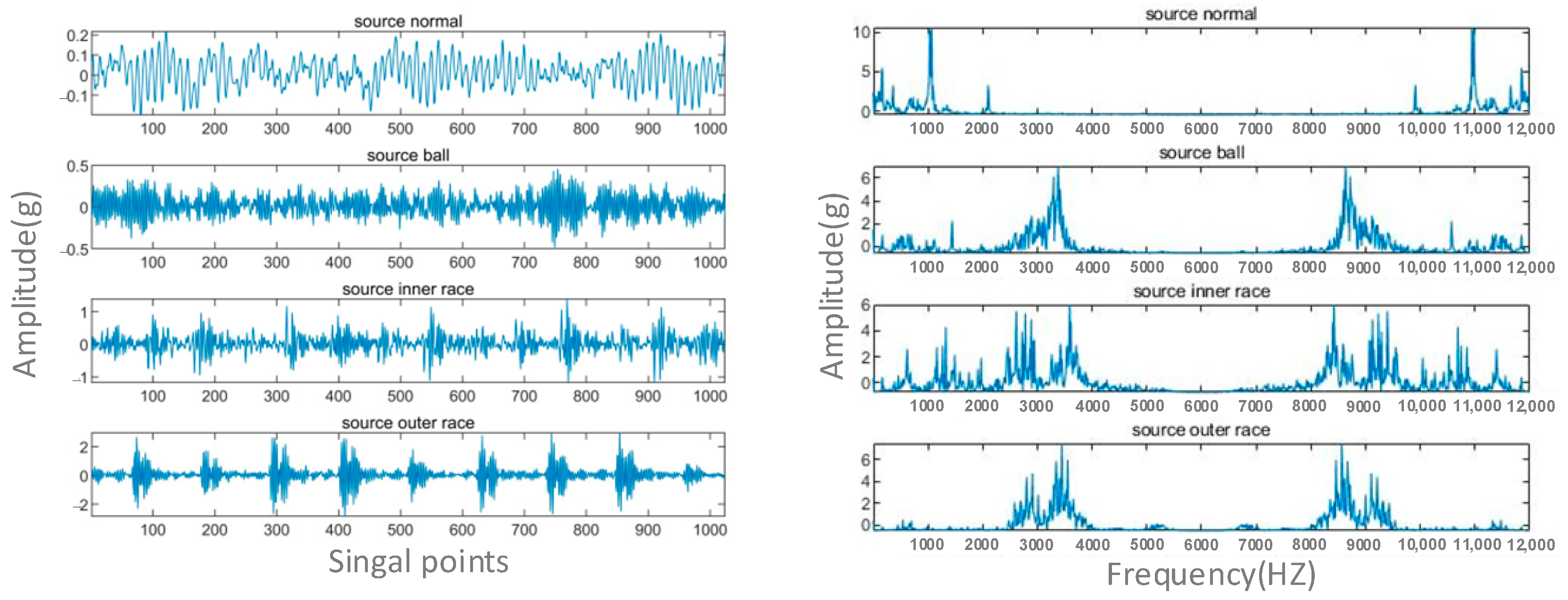
Effective preprocessing of vibration signals enhances the extraction of insightful features via deep networks. Certain researchers have employed the Fast Fourier Transform (FFT) on the raw signals, obtaining their spectra as inputs for deep networks aimed at alleviating the impact of noise [7,49,50]. Figure 6 illustrates time and frequency domain waveforms of bearing vibration data under distinct health states: (1) in the normal state, data predominantly exhibit smooth random waveforms characterized by minor amplitude fluctuations; (2) as indicated by Figure 6, noticeable periodic shocks and irregularities manifest in the data related to inner and outer ring failures, while such attributes are less conspicuous in instances of rolling element failures. Examination of the frequency domain waveforms yields the subsequent findings: (1) normal data demonstrate pronounced energy concentration primarily within the low and mid-frequency bands (below 1 kHz); (2) pertaining to data from other fault states, a distinct resemblance in the amplitude variation pattern is discernible, characterized by a dominant energy concentration in the high frequency range (2, 4 kHz).

4.1.3. Signal Reconstruction and Feature Extraction

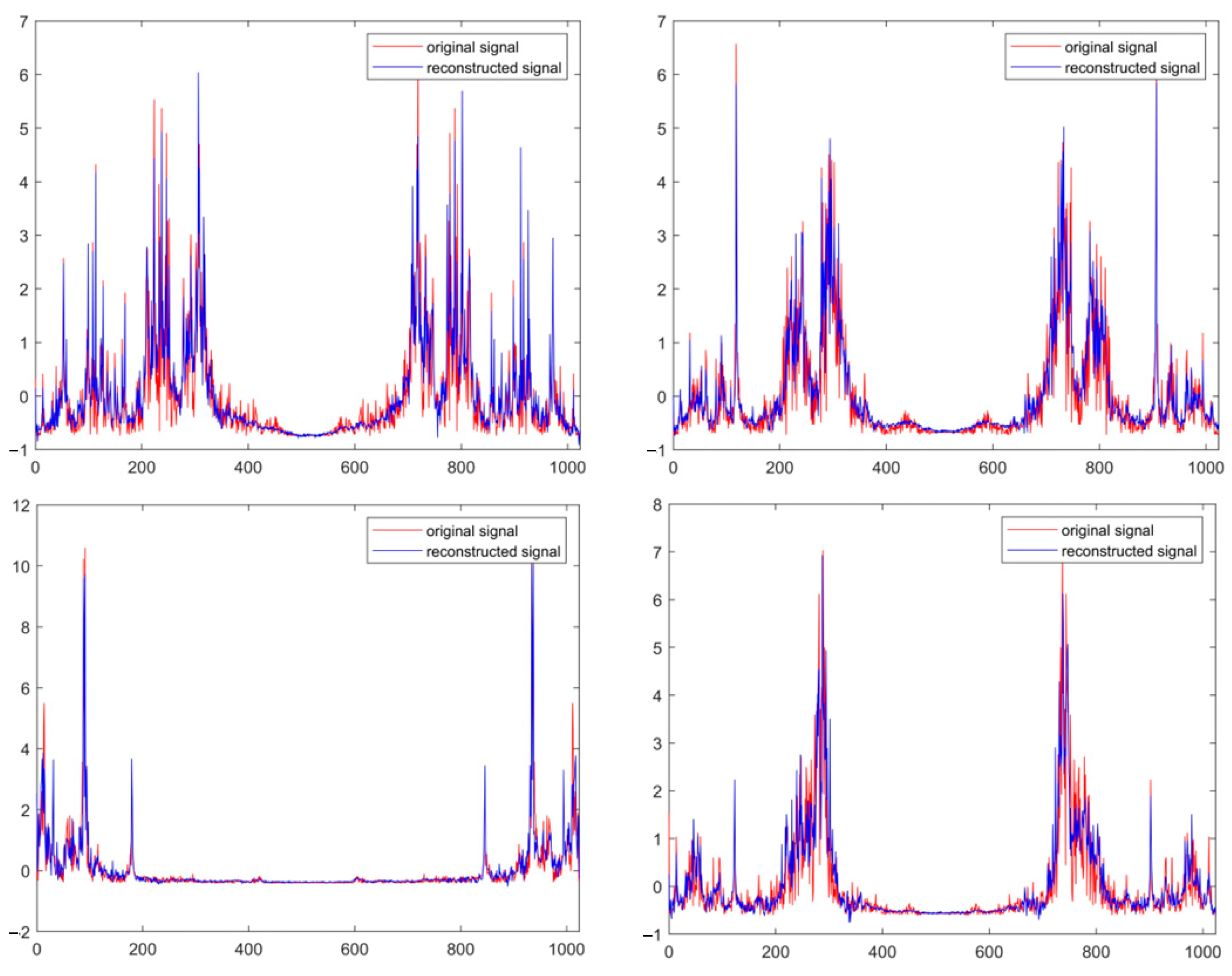
The convolutional autoencoder reconstructs input data by acquiring a condensed representation and subsequently generating a reconstruction using this representation. The primary objective of data reconstruction lies in distilling the most valuable information from the input while minimizing noise and redundancy. The outcomes, illustrated in Figure 7, demonstrate that the training of the autoencoder is highly efficacious. The reconstructed signal adeptly emulates the original waveform, showcasing precise reconstruction.
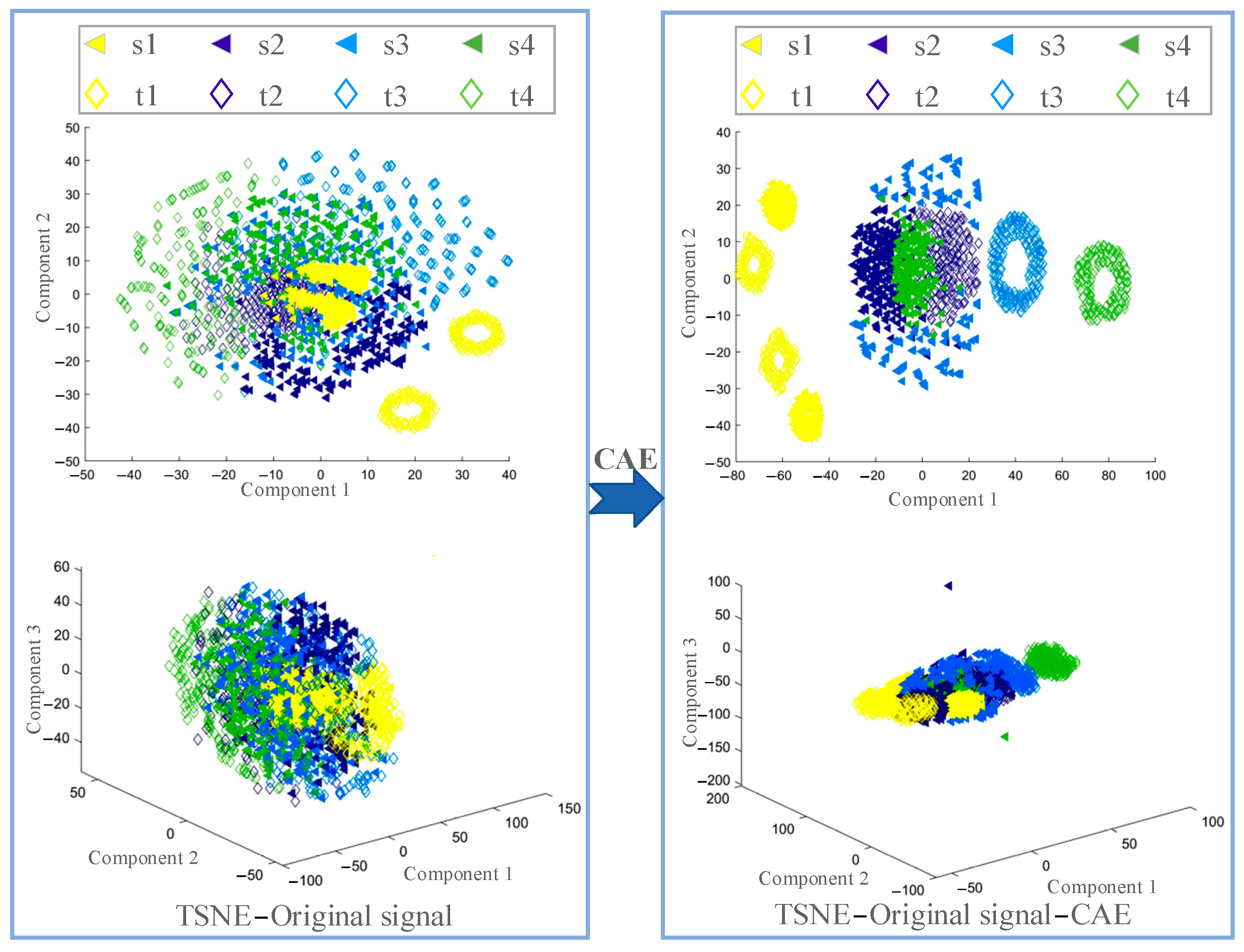
To further elucidate the efficacy of the CAE, we employed the t-sne algorithm to visualize feature distributions. Importantly, in order to underscore the importance of data preprocessing, we fed both the FFT spectrum sample and the original vibration signal sample individually into the CAE. From the encoder, we derived the resultant features and utilized the t-sne technique to diminish their dimensionality and observe their distribution patterns. The original vibration signal is subjected to feature extraction via CAE and subsequently transformed into two- and three-dimensional feature distributions through t-sne, as illustrated in Figure 8.
As depicted in the figure, the feature distribution of the original signal (TSNE-Original signal) appears disordered, with various fault types intermingled and lacking distinguishability. This observation implies that the original data fail to elucidate the latent features associated with distinct labels. Following the CAE-based learning of implied features and subsequent dimensionality reduction (TSNE-Original signal-CAE), the features related to different fault types demonstrated an initial level of differentiation. Nonetheless, the distinction between diverse labels remained somewhat indistinct. This suggests that the original vibration signal, subsequent to CAE learning, can manifest the latent features corresponding to different labels to some extent.
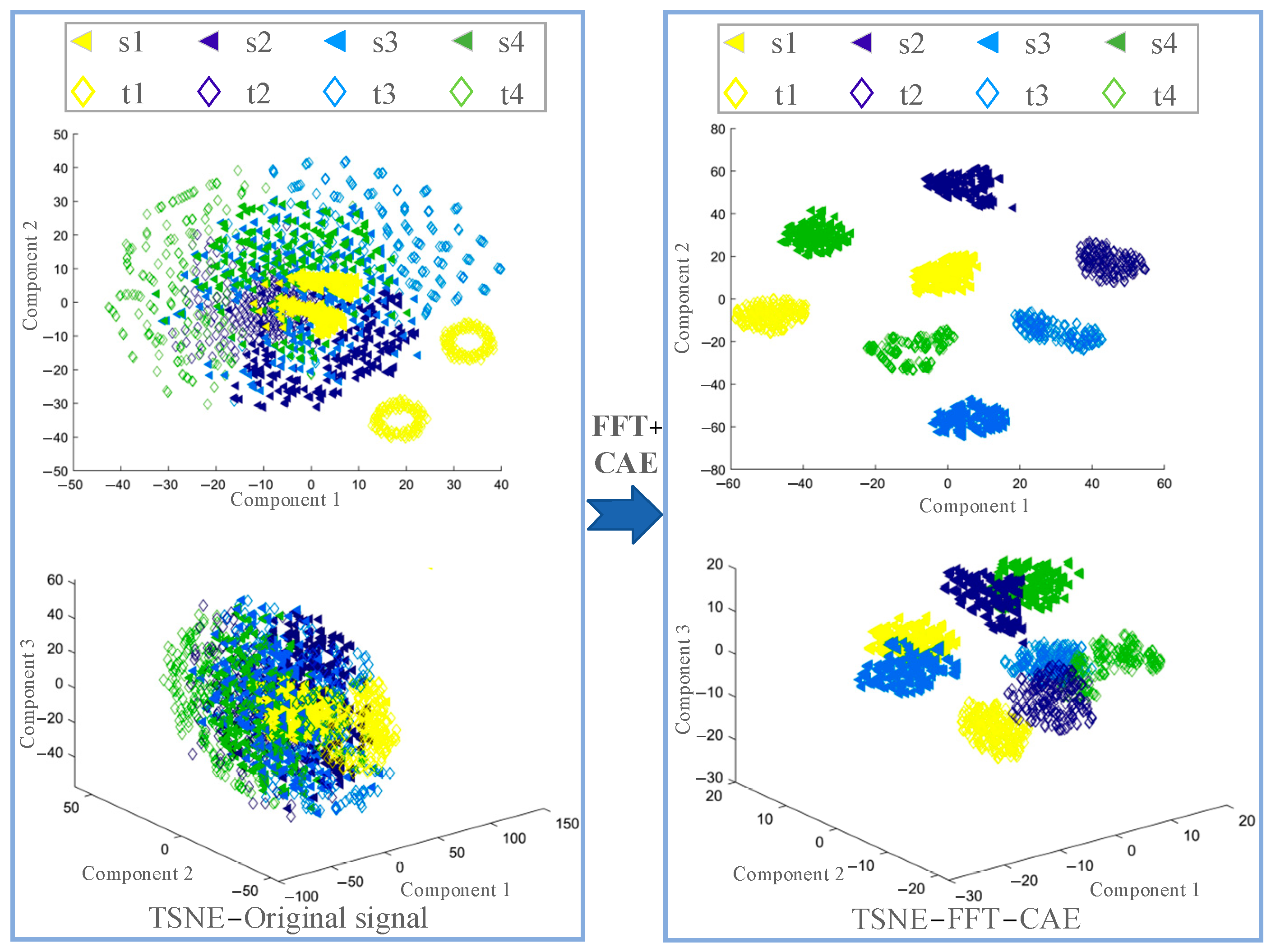
The FFT spectrum samples were input into a convolutional auto-encoder (CAE), which employs its encoder to generate latent features. These derived features subsequently undergo t-SNE-based dimensionality reduction, yielding both two- and three-dimensional visualizations, as depicted in Figure 9. Following the encoding step, feature data that share the same labels displayed prominent resemblances, particularly within the two-dimensional space. This outcome yielded a clustering effect of significantly higher quality than the one displayed in Figure 8. By combining insights from Figure 8 and Figure 9, it becomes evident that the CAE possesses a robust capability for profound feature extraction, thereby uncovering the latent characteristics of the signal. Furthermore, the indispensable nature of FFT preprocessing on the original signal is underscored.

4.1.4. Feature Migration and Analysis

As depicted in Figure 9, diverse fault types within the source domain exhibited a prominent clustering phenomenon, with the two-dimensional visualization particularly accentuating this effect. However, when the same faults manifest across diverse domains, the anticipated clustering patterns did not emerge. This discrepancy poses challenges in effectively diagnosing faults amidst differing operational contexts. Hence, we introduced an unsupervised domain adaptation migration technique grounded in BDA. The objective of this technique is to facilitate the transfer of identical fault characteristics across disparate domains, ultimately augmenting the diagnostic process supported by the classifier.
Source domain: normal and three fault data at 0 HP, fault diameter 0.007 inch D S = { n o r m a l , b a l l , i r , o r } 0.007 .
Target domain: normal and three fault data at 3 HP with a fault diameter of 0.014 inches D t = { n o r m a l , b a l l , i r , o r } 0.014 .
Task: Migration of untagged data in the target domain using the already tagged source domain data.
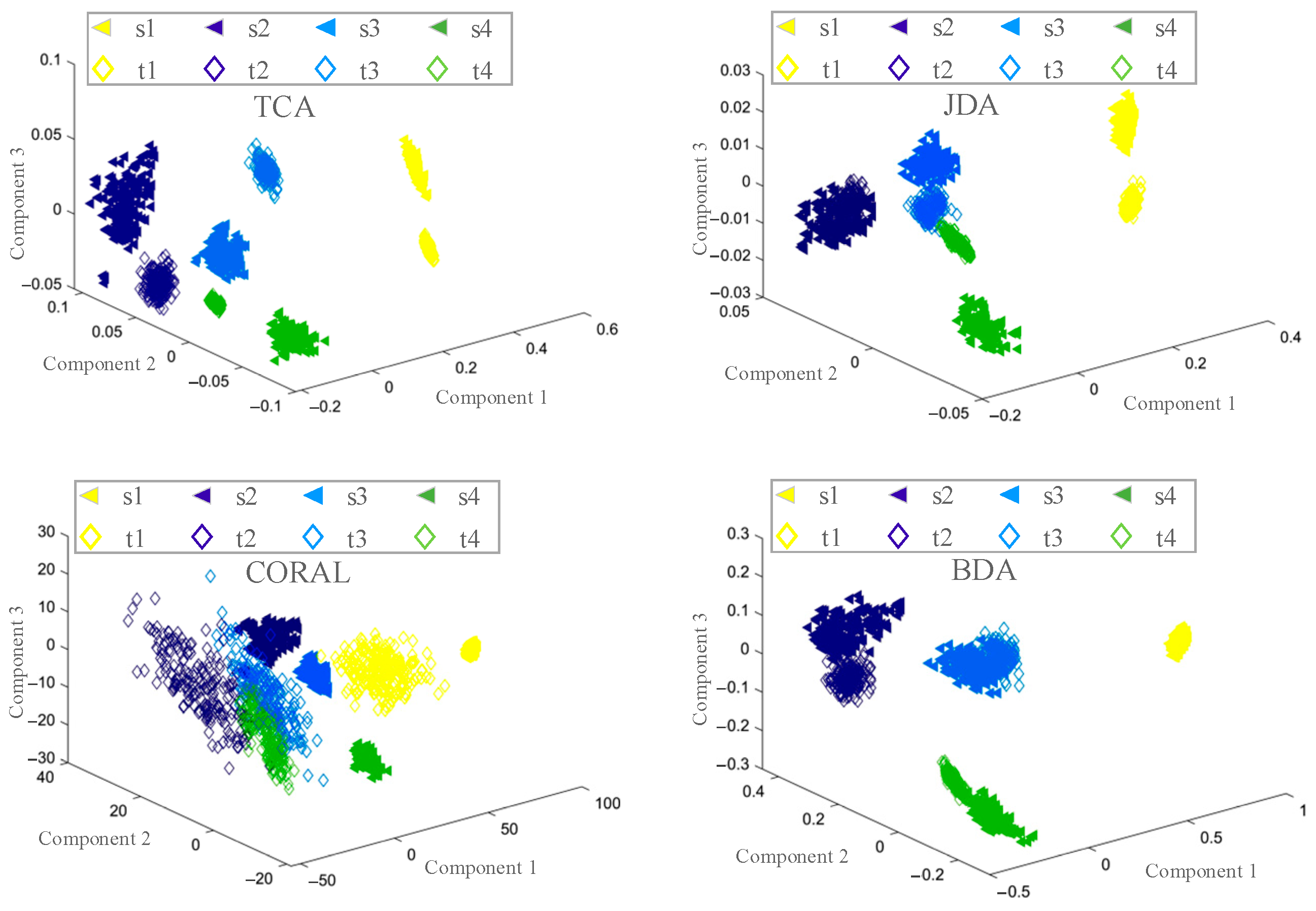
The FFT spectrum serves as the input to the CAE, with the encoder generating implied features. Subsequently, the source and target domain features underwent migration through algorithms such as TCA, JDA, CORAL and BDA. These migrated features were then reduced to a three-dimensional space using the t-sne technique, facilitating the observation of clustering effects. The outcomes are presented in Figure 10.
In Figure 10, we present the migration outcomes resulting from the TCA, JDA, CORAL, and BDA migration algorithms, respectively. Contrasting with Figure 8, the TCA algorithm bolstered the clustering efficacy of each label. However, it falls short in effectively bridging the gap between the source and target domains, and its migration outcomes are suboptimal. Comparatively, the JDA algorithm slightly outperformed the TCA algorithm, exhibiting a commendable migration impact on label No. 2. The CORAL algorithm, in contrast, manifested the least successful migration results. The BDA algorithm’s migration outcomes, on the other hand, stand out. Under the purview of the BDA algorithm, labels sharing the same category across source and target domains were aptly grouped together, concurrently ensuring distinctiveness among disparate labels. This achievement underscores the method’s efficacy in ameliorating data distribution disparities across distinct domains.

4.1.5. Fault Classification and Analysis

In this segment, we enhanced the comparison by integrating various feature types and classification algorithms to underscore the superior attributes of the proposed technique. Initially, FFT spectral features were derived through the CAE. Subsequently, feature migration transpires via TCA, JDA, CORAL, and BDA migration algorithms. Ultimately, the realm of fault classification is navigated through a composite strategy integrating well-established KNN, SVM, and GBDT classifiers. Additionally, we introduced four supplementary approaches: DFCNN, CAE-DTLN [51], 1DRCAE [52] (deep learning algorithms) and DEEP FEATURE-KNN (directly utilizing the KNN algorithm to classify the features extracted by means of the CAE). This amalgamation culminates in a total of eleven distinct methodologies.
(1)
TCA-KNN
(2)
TCA-GBDT
(3)
CORAL-KNN
(4)
JDA-KNN
(5)
BDA-KNN
(6)
BDA-SVM
(7)
BDA-GBDT
(8)
DFCNN
(9)
DEEP FEATURE-KNN
(10)
CAE-DTLN
(11)
1DRCAE
The experimental outcomes are showcased in Table 3 and Figure 11, derived from 10 replicate trials. Evaluation metrics encompass the mean accuracy and standard deviation.
Observing Table 3 along with Figure 11 and Figure 12, it becomes evident that the proposed BDA-KNN method attained the highest mean accuracy and nearly the lowest standard deviation. Conversely, CORAL-KNN exhibited the lowest standard deviation but poor accuracy performance. In summary, these findings highlight the superior performance of BDA-KNN. Additionally, it is worth noting that the classification effectiveness substantially surpasses that of the CORAL algorithm when employing BDA, TCA, and JDA migration algorithms. This observation aligns with the feature visualization depicted in Figure 10. A more pronounced clustering effect between source and target domain features correlates with an easier fault diagnosis. Moreover, the majority of migration methods outperformed the deep learning algorithms DFCNN, CAE-DTLN, 1DRCAE, and DEEP FEATURE-KNN, which rely solely on CAE depth features for diagnosis. This underscores the ascendancy of migration learning in cross-service fault diagnosis.
To provide a visually illustrative depiction of the proposed method’s performance, Figure 11 presents the confusion matrix based on the CWRU dataset. The figure demonstrates the model’s robust diagnostic proficiency across all categories of fault types.

4.2. Southeastern University Gearbox Dataset

4.2.1. Data Description

Bearing data were acquired from the drivetrain dynamics simulator (DDS), as depicted in Figure 13.
As depicted in Table 4, we investigated two distinct operational scenarios, wherein the rotation speed-system load configurations were set to 20 Hz-0 V and 30 Hz-2 V, respectively.

4.2.2. Signal Pre-Processing

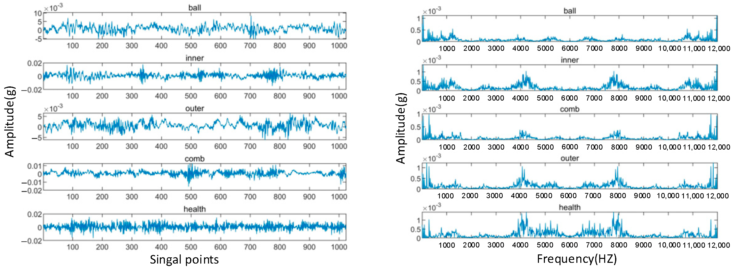
Figure 14 depicted the time and frequency-domain waveforms of bearing vibration data across distinct health conditions: (1) for normal conditions, the data predominantly exhibit smooth random waveforms characterized by minor amplitude fluctuations; and (2) as illustrated in Figure 14, conspicuous burrs and irregular waveforms manifest in the data linked to inner and outer ring failures, while such features are less noticeable in instances of rolling element failures. The frequency domain waveforms reveal a predominant energy concentration within the high frequency range (4, 6 kHz).

4.2.3. Signal Reconstruction and Feature Extraction

The convolutional autoencoder reconstructs input data by acquiring a condensed representation and subsequently generating a reconstruction using this representation. The primary objective of data reconstruction lies in distilling the most valuable information from the input while minimizing noise and redundancy. The outcomes, illustrated in Figure 15, demonstrate that the training of the autoencoder is highly efficacious. The reconstructed signal adeptly emulates the original waveform, showcasing precise reconstruction.
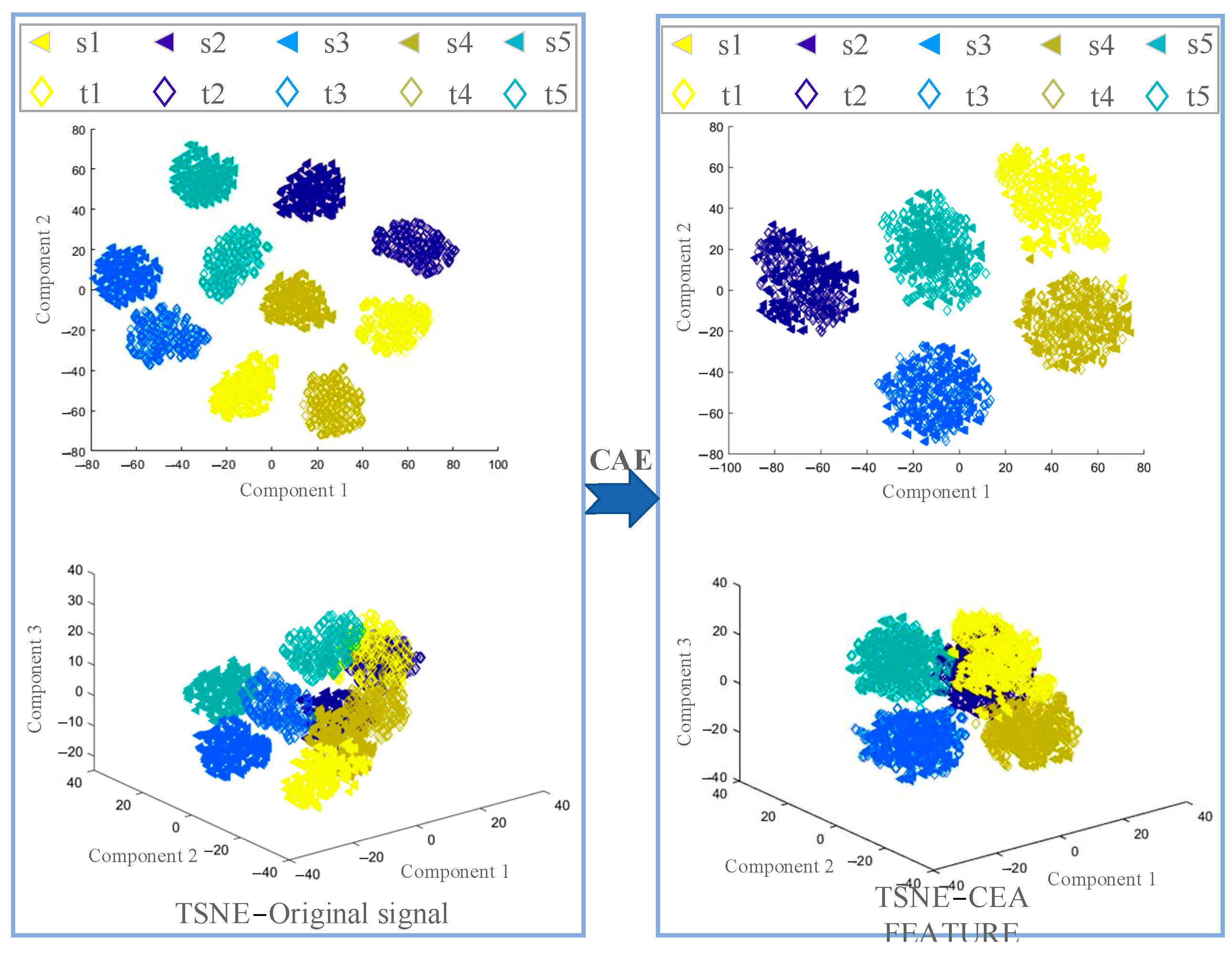
In a bid to bolster the persuasive efficacy, we additionally employ the t-sne algorithm to visualize the implied features extracted by the CAE. Furthermore, to underscore the indispensability of data pre-processing, we juxtaposed the feature distributions of the original data samples with those of the FFT spectrum samples. The ensuing comparison is depicted in Figure 16, wherein the feature distributions, reduced to both two and three dimensions through t-sne, are showcased.
Derived from Figure 16, it becomes apparent that direct dimensionality reduction applied to the original data resulted in a considerable overlap of features across all health states. This outcome underscores the incapacity of the original data to unveil the inherent patterns associated with fault types. On the other hand, feeding the raw data into the CAE for feature extraction, within both two and three-dimensional spaces, reveals nascent distinctions among various fault types. Nevertheless, the lingering challenge of feature overlap remains unaddressed.
As illustrated in Figure 17, the FFT spectrum samples underwent feature extraction within the CAE model, subsequently followed by t-sne visualization. This examination revealed a commendable clustering effect within both two and three-dimensional spaces. The comprehensive insights provided by Figure 15 underscore CAE’s adeptness in feature extraction, facilitating the acquisition of the inherent characteristics associated with various fault types. This visualization also underscores the essentiality of FFT pre-processing for the samples. The resultant features, transformed through FFT and subsequently extracted via the CAE, are henceforth denoted as “CAE features”.

4.2.4. Feature Migration

To substantiate the excellence of the BDA algorithm, four migration learning methodologies TCA, JDA, CORAL, and BDA were employed for migrating CAE features and investigating the ensuing feature clustering phenomenon. This analysis is depicted in Figure 18.
Observing the figure, it becomes evident that TCA effectively migrates tag types 3 and 4, yet displayed limited efficacy in migrating other tag types. JDA likewise exceled at migrating tag types 3 and 4, while demonstrating subpar performance for the remaining categories. On the other hand, CORAL exhibited the least desirable migration outcomes. BDA, conversely, delivered commendable performance across all tag types, thereby conferring strong discriminability among them. Notably, BDA’s proficiency in migrating features between the source and target domains underscores its remarkable domain adaptation capabilities.

4.2.5. Fault Classification and Analysis

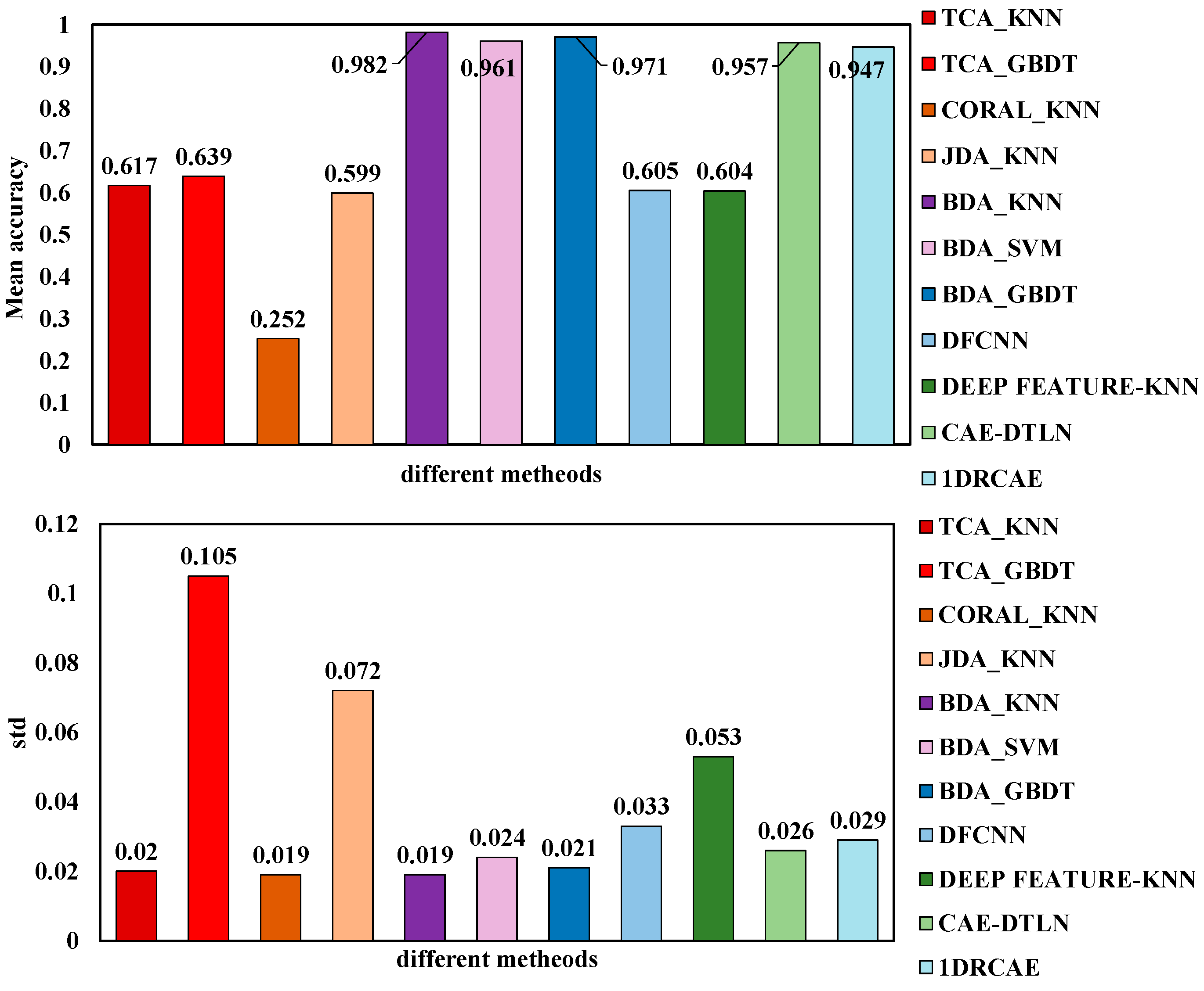
In alignment with the CWRU dataset, an identical algorithm was employed for comparison purposes. The experiment was replicated 10 times, with the average diagnostic accuracy and standard deviation (STD) serving as the evaluation metrics. The outcomes are visually depicted in Figure 19 and tabulated in Table 5.
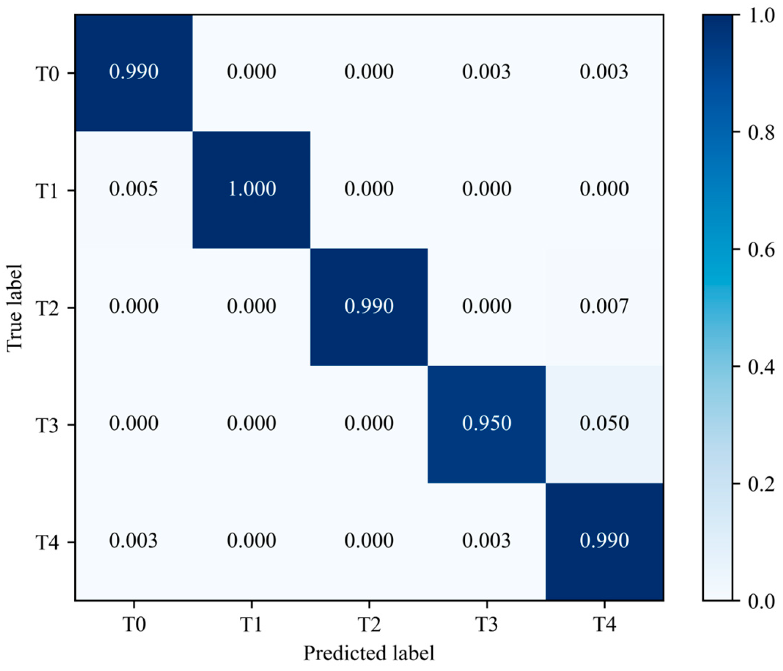
As Table 5 and Figure 19 and Figure 20 demonstrate, it is clear that the proposed BDA-KNN method has achieved the highest mean accuracy and almost the lowest standard deviation. In contrast, CORAL-KNN displayed the lowest standard deviation, but poor accuracy performance. To sum up, these results underscore the superior performance of BDA-KNN. Furthermore, it is noteworthy that the classification effectiveness significantly exceeds that of the CORAL algorithm when employing BDA, TCA, and JDA migration algorithms. This observation is consistent with the feature visualization presented in Figure 18. A stronger clustering effect among source and target domain features corresponds to easier fault diagnosis. Moreover, the majority of migration methods outperformed deep learning algorithms such as DFCNN, CAE-DTLN, 1DRCAE, and DEEP FEATURE-KNN, which rely solely on CAE depth features for diagnosis. This highlights the superiority of migration learning in cross-service fault diagnosis.
For a more visual portrayal of the diagnostic accuracy attributed to the suggested approach, Figure 20 delineates the confusion matrix over the SEU dataset. The visualization demonstrates the model’s adeptness in fault diagnosis across all fault types.
In summary, the BDA-KNN method presented in this paper demonstrates a notably high average accuracy and a minimal standard deviation when compared to alternative approaches. Furthermore, this method exhibits remarkable migration results. Utilizing BDA, it effectively combines labels of the same categories from the source and target data sources while preserving the differentiation between distinct labels. This method effectively mitigates data distribution disparities across diverse domains.

5. Conclusions

This article presents an unsupervised domain adaptive approach for the cross-condition diagnosis of bearings. The methodology leverages convolutional auto-encoders (CAEs) to extract intricate features from vibration signals, enabling the subsequent application of the balancing domain adaptation (BDA) algorithm. This algorithm facilitates the unsupervised migration of extracted features between the source and target domains, without necessitating target domain labeling. The BDA algorithm achieves this by intelligently weighing the significance of inter-domain edge distribution and conditional distribution. Ultimately, the diagnosis of rolling bearing faults across varied working conditions is achieved using the K-nearest neighbor (KNN) algorithm. To validate the methodology’s efficacy, changes in data distribution during feature extraction and migration were reproduced through the utilization of the t-SNE technique, which further verified the heightened diagnostic prowess of the proposed approach. Furthermore, the performance of the approach was validated across diverse datasets, with the ensuing experimental results concretely confirming the effectiveness and superiority of the method.
Nevertheless, considering that domain adaptation methods are often sensitive to disparities in data distribution, the methods introduced in this paper possessed certain limitations. The domain adaptation approach proposed in this paper was grounded on the assumption of distinct operational circumstances for the same equipment, exhibiting commendable generalization and resilience in the face of varied working conditions for the same equipment. However, there remains a considerable scope for enhancing the model’s efficacy in adapting between different devices. Consequently, our future endeavors will be centered on bolstering the generalization capacity and robustness of domain adaptation across diverse devices.

Author Contributions

Methodology, W.M.; Writing—original draft, Z.Z. and H.L.; Writing—review & editing, Z.Z.; Visualization, Y.C.; Project administration, X.X.; Funding acquisition, Z.Z. All authors have read and agreed to the published version of the manuscript.

Funding

This project was supported by the Henan Province Major Science and Technology Special Project (No. 221100220100) and the Henan Provincial Science and Technology Research and Development Joint Fund Project (No. 222103810030).

Data Availability Statement

Conflicts of Interest

The authors declare no conflict of interest.

Nomenclature

AEautoencoder
BDAbalanced distribution adaption
CNNconvolutional neural network
DFTdiscrete Fourier transform
FFTfast Fourier transform
GANgenerative adversarial network
KNNK-nearest neighbor
MMDmaximum mean discrepancy
T-SNET-distributed stochastic neighbor embedding
D S source domain space
D t target domain space
X ( k ) spectral function
X ^ output of decoder
l A E reconstruction error
p ( x ) marginal distribution
p ( y | x ) conditional distribution
μ balance factor
κ regenerative kernel Hilbert space
Hcentral matrix
Iunit matrix
Atransformation matrix
ϕ Lagrangian operator

References

  1. Zhang, S.; Wang, B.; Habetler, T.G. Deep Learning Algorithms for Bearing Fault Diagnostics—A Comprehensive Review. IEEE Access 2020, 8, 29857–29881. [Google Scholar] [CrossRef]
  2. Liu, Z.-H.; Meng, X.-D.; Wei, H.-L.; Chen, L.; Lu, B.-L.; Wang, Z.-H.; Chen, L. A Regularized LSTM Method for Predicting Remaining Useful Life of Rolling Bearings. Int. J. Autom. Comput. 2021, 18, 581–593. [Google Scholar] [CrossRef]
  3. Neupane, D.; Seok, J. Bearing Fault Detection and Diagnosis Using Case Western Reserve University Dataset with Deep Learning Approaches: A Review. IEEE Access 2020, 8, 93155–93178. [Google Scholar] [CrossRef]
  4. Rai, A.; Upadhyay, S. A review on signal processing techniques utilized in the fault diagnosis of rolling element bearings. Tribol. Int. 2016, 96, 289–306. [Google Scholar] [CrossRef]
  5. Benali, J.; Sayadi, M.; Fnaiech, F.; Morello, B.; Zerhouni, N. Importance of the fourth and fifth intrinsic mode functions for bearing fault diagnosis. In Proceedings of the 14th International Conference on Sciences and Techniques of Automatic Control & Computer Engineering—STA’2013, Sousse, Tunisia, 20–22 December 2013; pp. 259–264. [Google Scholar] [CrossRef]
  6. Peng, B.; Bi, Y.; Xue, B.; Zhang, M.; Wan, S. A Survey on Fault Diagnosis of Rolling Bearings. Algorithms 2022, 15, 347. [Google Scholar] [CrossRef]
  7. Xie, W.; Li, Z.; Xu, Y.; Gardoni, P.; Li, W. Evaluation of Different Bearing Fault Classifiers in Utilizing CNN Feature Extraction Ability. Sensors 2022, 22, 3314. [Google Scholar] [CrossRef]
  8. Cerrada, M.; Sánchez, R.-V.; Li, C.; Pacheco, F.; Cabrera, D.; de Oliveira, J.V.; Vásquez, R.E. A review on data-driven fault severity assessment in rolling bearings. Mech. Syst. Signal Process. 2018, 99, 169–196. [Google Scholar] [CrossRef]
  9. Chen, Z.; Xu, J.; Alippi, C.; Ding, S.X.; Shardt, Y.; Peng, T.; Yang, C. Graph neural network-based fault diagnosis: A review. arXiv 2021, arXiv:2111.08185. [Google Scholar]
  10. Liu, Z.-H.; Jiang, L.-B.; Wei, H.-L.; Chen, L.; Li, X.-H. Optimal Transport Based Deep Domain Adaptation Approach for Fault Diagnosis of Rotating Machine. IEEE Trans. Instrum. Meas. 2021, 70, 1–12. [Google Scholar] [CrossRef]
  11. Li, H.; Lian, X.; Guo, C.; Zhao, P. Investigation on early fault classification for rolling element bearing based on the optimal frequency band determination. J. Intell. Manuf. 2013, 26, 189–198. [Google Scholar] [CrossRef]
  12. Singh, D.S.; Zhao, Q. Pseudo-fault signal assisted EMD for fault detection and isolation in rotating machines. Mech. Syst. Signal Process. 2016, 81, 202–218. [Google Scholar] [CrossRef]
  13. Wang, J.; He, Q. Wavelet Packet Envelope Manifold for Fault Diagnosis of Rolling Element Bearings. IEEE Trans. Instrum. Meas. 2016, 65, 2515–2526. [Google Scholar] [CrossRef]
  14. Osman, S.; Wang, W. A Morphological Hilbert-Huang Transform Technique for Bearing Fault Detection. IEEE Trans. Instrum. Meas. 2016, 65, 2646–2656. [Google Scholar] [CrossRef]
  15. Lei, Y.; Lin, J.; He, Z.; Zuo, M.J. A review on empirical mode decomposition in fault diagnosis of rotating machinery. Mech. Syst. Signal Process. 2013, 35, 108–126. [Google Scholar] [CrossRef]
  16. Dragomiretskiy, K.; Zosso, D. Variational Mode Decomposition. IEEE Trans. Signal Process. 2014, 62, 531–544. [Google Scholar] [CrossRef]
  17. Wang, X.; Sui, G.; Xiang, J.; Wang, G.; Huo, Z.; Huang, Z. Multi-Domain Extreme Learning Machine for Bearing Failure Detection Based on Variational Modal Decomposition and Approximate Cyclic Correntropy. IEEE Access 2020, 8, 197711–197729. [Google Scholar] [CrossRef]
  18. Wang, F.; Dun, B.; Liu, X.; Xue, Y.; Li, H.; Han, Q. An Enhancement Deep Feature Extraction Method for Bearing Fault Diagnosis Based on Kernel Function and Autoencoder. Shock Vib. 2018, 2018, 6024874. [Google Scholar] [CrossRef]
  19. Zhang, X.; Wang, B.; Chen, X. Intelligent fault diagnosis of roller bearings with multivariable ensemble-based incremental support vector machine. Knowl.-Based Syst. 2015, 89, 56–85. [Google Scholar] [CrossRef]
  20. Huo, Z.; Martinez-Garcia, M.; Zhang, Y.; Yan, R.; Shu, L. Entropy Measures in Machine Fault Diagnosis: Insights and Applications. IEEE Trans. Instrum. Meas. 2020, 69, 2607–2620. [Google Scholar] [CrossRef]
  21. Li, C.; Zheng, J.; Pan, H.; Tong, J.; Zhang, Y. Refined Composite Multivariate Multiscale Dispersion Entropy and Its Application to Fault Diagnosis of Rolling Bearing. IEEE Access 2019, 7, 47663–47673. [Google Scholar] [CrossRef]
  22. Jiao, W.; Li, G.; Jiang, Y.; Baim, R.; Tang, C.; Yan, T.; Ding, X.; Yan, Y. Multi-Scale Sample Entropy-Based Energy Moment Features Applied to Fault Classification. IEEE Access 2021, 9, 8444–8454. [Google Scholar] [CrossRef]
  23. Mushtaq, S.; Islam, M.M.M.; Sohaib, M. Deep Learning Aided Data-Driven Fault Diagnosis of Rotatory Machine: A Comprehensive Review. Energies 2021, 14, 5150. [Google Scholar] [CrossRef]
  24. Malhi, A.; Gao, R. PCA-Based Feature Selection Scheme for Machine Defect Classification. IEEE Trans. Instrum. Meas. 2004, 53, 1517–1525. [Google Scholar] [CrossRef]
  25. Yang, Y.; Yu, D.; Cheng, J. A fault diagnosis approach for roller bearing based on IMF envelope spectrum and SVM. Measurement 2007, 40, 943–950. [Google Scholar] [CrossRef]
  26. Shen, F.; Chen, C.; Yan, R.; Gao, R.X. Bearing fault diagnosis based on SVD feature extraction and transfer learning classification. In Proceedings of the 2015 Prognostics and System Health Management Conference (PHM), Beijing, China, 21–23 October 2015. [Google Scholar]
  27. Zhang, N.; Wu, L.; Yang, J.; Guan, Y. Naive Bayes Bearing Fault Diagnosis Based on Enhanced Independence of Data. Sensors 2018, 18, 463. [Google Scholar] [CrossRef]
  28. Jia, F.; Lei, Y.; Lin, J.; Zhou, X.; Lu, N. Deep neural networks: A promising tool for fault characteristic mining and intelligent diagnosis of rotating machinery with massive data. Mech. Syst. Signal Process. 2016, 72–73, 303–315. [Google Scholar] [CrossRef]
  29. Xia, M.; Li, T.; Xu, L.; Liu, L.; de Silva, C.W. Fault Diagnosis for Rotating Machinery Using Multiple Sensors and Convolutional Neural Networks. IEEE/ASME Trans. Mechatron. 2017, 23, 101–110. [Google Scholar] [CrossRef]
  30. Shao, H.; Jiang, H.; Wang, F.; Wang, Y. Rolling bearing fault diagnosis using adaptive deep belief network with dual-tree complex wavelet packet. ISA Trans. 2017, 69, 187–201. [Google Scholar] [CrossRef]
  31. Sun, W.; Shao, S.; Zhao, R.; Yan, R.; Zhang, X.; Chen, X. A sparse auto-encoder-based deep neural network approach for induction motor faults classification. Measurement 2016, 89, 171–178. [Google Scholar] [CrossRef]
  32. Kerboua, A.; Kelaiaia, R. Fault Diagnosis in an Asynchronous Motor Using Three-Dimensional Convolutional Neural Network. Arab. J. Sci. Eng. 2023, 1–19. [Google Scholar] [CrossRef]
  33. Liang, B.; Feng, W. Bearing Fault Diagnosis Based on ICEEMDAN Deep Learning Network. Processes 2023, 11, 2440. [Google Scholar] [CrossRef]
  34. Ma, P.; Zhang, H.; Fan, W.; Wang, C. A diagnosis framework based on domain adaptation for bearing fault diagnosis across diverse domains. ISA Trans. 2019, 99, 465–478. [Google Scholar] [CrossRef] [PubMed]
  35. Li, X.; Zhang, W.; Ding, Q.; Sun, J.-Q. Multi-Layer domain adaptation method for rolling bearing fault diagnosis. Signal Process. 2018, 157, 180–197. [Google Scholar] [CrossRef]
  36. Xu, W.; Wan, Y.; Zuo, T.-Y.; Sha, X.-M. Transfer Learning Based Data Feature Transfer for Fault Diagnosis. IEEE Access 2020, 8, 76120–76129. [Google Scholar] [CrossRef]
  37. Lu, W.; Liang, B.; Cheng, Y.; Meng, D.; Yang, J.; Zhang, T. Deep Model Based Domain Adaptation for Fault Diagnosis. IEEE Trans. Ind. Electron. 2016, 64, 2296–2305. [Google Scholar] [CrossRef]
  38. Li, M.; Sun, Z.-H.; He, W.; Qiu, S.; Liu, B. Rolling Bearing Fault Diagnosis under Variable Working Conditions Based on Joint Distribution Adaptation and SVM. In Proceedings of the 2020 International Joint Conference on Neural Networks (IJCNN), Glasgow, UK, 19–24 July 2020; pp. 1–8. [Google Scholar] [CrossRef]
  39. Wang, J.; Chen, Y.; Hao, S.; Feng, W.; Shen, Z. Balanced Distribution Adaptation for Transfer Learning. In Proceedings of the 2017 IEEE International Conference on Data Mining (ICDM), New Orleans, LA, USA, 18–21 November 2017. [Google Scholar]
  40. Welaratna, S. Thirty Years of FFT Analyzers; Sound and Vibration: San Jose, CA, USA, 1997. [Google Scholar]
  41. Hakim, M.; Omran, A.A.B.; Inayat-Hussain, J.I.; Ahmed, A.N.; Abdellatef, H.; Abdellatif, A.; Gheni, H.M. Bearing Fault Diagnosis Using Lightweight and Robust One-Dimensional Convolution Neural Network in the Frequency Domain. Sensors 2022, 22, 5793. [Google Scholar] [CrossRef]
  42. Zhang, M.; Yin, J.; Chen, W. Rolling Bearing Fault Diagnosis Based on Time-Frequency Feature Extraction and IBA-SVM. IEEE Access 2022, 10, 85641–85654. [Google Scholar] [CrossRef]
  43. Mao, W.; Liu, Y.; Ding, L.; Li, Y. Imbalanced Fault Diagnosis of Rolling Bearing Based on Generative Adversarial Network: A Comparative Study. IEEE Access 2019, 7, 9515–9530. [Google Scholar] [CrossRef]
  44. Hinton, G.E.; Salakhutdinov, R.R. Reducing the Dimensionality of Data with Neural Networks. Science 2006, 313, 504–507. [Google Scholar] [CrossRef]
  45. Mao, W.; Chen, J.; Liang, X.; Zhang, X. A New Online Detection Approach for Rolling Bearing Incipient Fault via Self-Adaptive Deep Feature Matching. IEEE Trans. Instrum. Meas. 2019, 69, 443–456. [Google Scholar] [CrossRef]
  46. An, J.; Ai, P.; Liu, C.; Xu, S.; Liu, D. Deep Clustering Bearing Fault Diagnosis Method Based on Local Manifold Learning of an Autoencoded Em-bedding. IEEE Access 2021, 9, 30154–30168. [Google Scholar] [CrossRef]
  47. Lecun, Y.; Bottou, L.; Bengio, Y.; Haffner, P. Gradient-based learning applied to document recognition. Proc. IEEE 1998, 86, 2278–2324. [Google Scholar] [CrossRef]
  48. Lei, Y.; Yang, B.; Jiang, X.; Jia, F.; Li, N.; Nandi, A.K. Applications of machine learning to machine fault diagnosis: A review and roadmap. Mech. Syst. Signal Process. 2020, 138, 106587. [Google Scholar] [CrossRef]
  49. Mao, W.; Liu, Y.; Ding, L.; Safian, A.; Liang, X. A New Structured Domain Adversarial Neural Network for Transfer Fault Diagnosis of Rolling Bearings Under Different Working Conditions. IEEE Trans. Instrum. Meas. 2020, 70, 1–13. [Google Scholar] [CrossRef]
  50. Liu, Z.-H.; Lu, B.-L.; Wei, H.-L.; Li, X.-H.; Chen, L. Fault Diagnosis for Electromechanical Drivetrains Using a Joint Distribution Optimal Deep Domain Adaptation Approach. IEEE Sens. J. 2019, 19, 12261–12270. [Google Scholar] [CrossRef]
  51. Qian, Q.; Qin, Y.; Wang, Y.; Liu, F. A new deep transfer learning network based on convolutional auto-encoder for mechanical fault diagnosis. Measurement 2021, 178, 109352. [Google Scholar] [CrossRef]
  52. Yu, J.; Zhou, X. One-Dimensional Residual Convolutional Autoencoder Based Feature Learning for Gearbox Fault Diagnosis. IEEE Trans. Ind. Inform. 2020, 16, 6347–6358. [Google Scholar] [CrossRef]
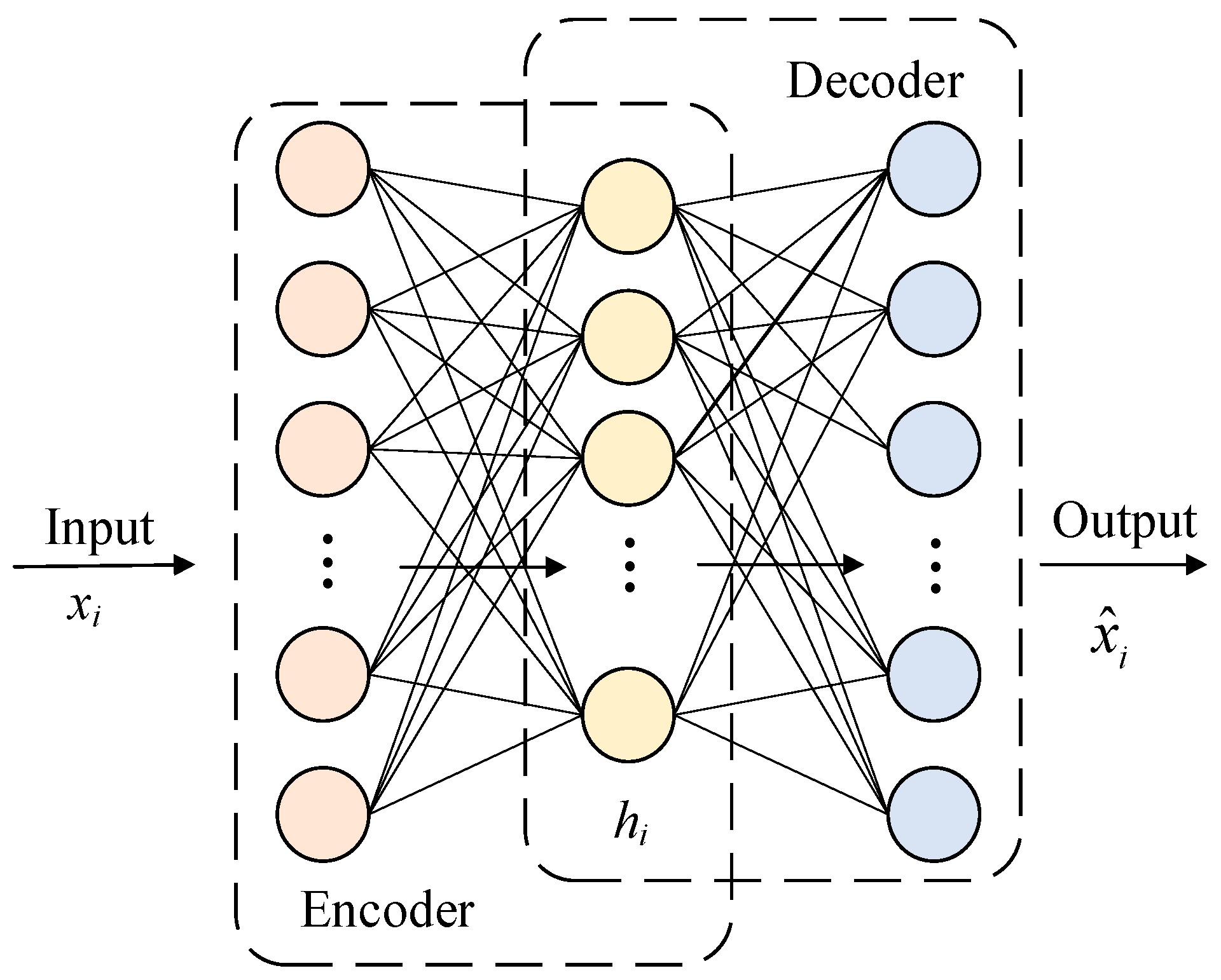
Figure 1. Structure of the AE.
Lubricants 11 00383 g001
Figure 2. Structure of the CNN.
Lubricants 11 00383 g002
Figure 3. Network structure of the CAE.
Lubricants 11 00383 g003
Figure 4. Unsupervised domain adaptation fault diagnosis framework.
Lubricants 11 00383 g004
Figure 5. CWRU experimental platform.
Lubricants 11 00383 g005
Figure 6. Illustration of vibration signals of the CWRU data set.
Lubricants 11 00383 g006
Figure 7. Reconstructed signal and original signal display.
Lubricants 11 00383 g007
Figure 8. Variation of feature distribution in raw CWRU datasets.
Lubricants 11 00383 g008
Figure 9. FFT spectral feature distribution variation diagram.
Lubricants 11 00383 g009
Figure 10. Comparison chart of the effect of different migration algorithms.
Lubricants 11 00383 g010
Figure 11. Histograms of the comparative results in Table 3.
Lubricants 11 00383 g011
Figure 12. Confusion matrix by the proposed method on the CWRU dataset.
Lubricants 11 00383 g012
Figure 13. Experimental setup for the gearbox dataset.
Lubricants 11 00383 g013
Figure 14. Southeastern University data set visualization.
Lubricants 11 00383 g014
Figure 15. Reconstructed data and original data on the Southeast University data set.
Lubricants 11 00383 g015
Figure 16. Variation of the feature distribution of the raw data.
Lubricants 11 00383 g016
Figure 17. FFT spectral feature distribution variation diagram.
Lubricants 11 00383 g017
Figure 18. Feature migration results of different migration algorithms.
Lubricants 11 00383 g018
Figure 19. Histograms of the comparative results in Table 5.
Lubricants 11 00383 g019
Figure 20. Confusion matrix by the proposed method on the Southeastern University dataset.
Lubricants 11 00383 g020
Table 1. Detailed configuration of the architecture for the CAE.
LayerTypeKernel Size/StrideOutput
InputData/1 × 1024
Conv1Convolution1d32/16128 × 16
PoolMaxPool2/264 × 16
Conv2Convolution1d3/164 × 32
PoolMaxPool2/232 × 32
Conv3Convolution1d3/132 × 64
PoolMaxPool2/216 × 64
Conv4Convolution1d3/116 × 64
PoolMaxPool2/28 × 64
Conv5Convolution1d3/16 × 64
PoolMaxPool2/23 × 64
UpsampleMaxUnpool2/26 × 64
Deconv1ConvTranspose1d3/18 × 64
UpsampleMaxUnpool2/216 × 64
Deconv2ConvTranspose1d3/116 × 64
UpsampleMaxUnpool2/232 × 64
Deconv3ConvTranspose1d3/132 × 32
UpsampleMaxUnpool2/264 × 32
Deconv4ConvTranspose1d3/164 × 16
Deconv5ConvTranspose1d3/11 × 1024
Table 2. Category information about the CWRU dataset.
ClassFaultDamage Diameter (inch)Load (HP)
Source1Normal0.0071
Source2Ball0.0071
Source3Inner0.0071
Source4Outer0.0071
Target1Normal0.0143
Target2Ball0.0143
Target3Inner0.0143
Target4Outer0.0143
Table 3. Accuracy and standard deviation of different methods on the CWEU dataset.
Evaluating IndicatorTCA_KNNTCA_GBDTCORAL_KNNJDA_KNNBDA_KNNBDA_SVMBDA_GBDTDFCNNDEEP FEATURE-KNNCAE-DTLN1DRCAE
Mean
accuracy
0.7760.4310.2560.8200.9850.9740.5360.6740.7040.9630.954
std0.0170.1160.0130.0580.0140.0180.0880.0360.0430.0210.024
Table 4. Bearing fault types description and data segmentation.
ClassFaultCondition
Source1Normal20 HZ-0 V
Source2Ball20 HZ-0 V
Source3Inner20 HZ-0 V
Source4Outer20 HZ-0 V
Source5Combination20 HZ-0 V
Target1Normal30 HZ-2 V
Target2Ball30 HZ-2 V
Target3Inner30 HZ-2 V
Target4Outer30 HZ-2 V
Target5Combination30 HZ-2 V
Table 5. Accuracy and standard deviation of different methods on the Southeastern University dataset.
Evaluating IndicatorTCA_KNNTCA_GBDTCORAL_KNNJDA_KNNBDA_KNNBDA_SVMBDA_GBDTDFCNNDEEP FEATURE-KNNCAE-DTLN1DRCAE
Mean
accuracy
0.6170.6390.2520.5990.9820.9610.9710.6050.6040.9570.947
std0.0200.1050.0190.0720.0190.0240.0210.0330.0530.0260.029
Disclaimer/Publisher’s Note: The statements, opinions and data contained in all publications are solely those of the individual author(s) and contributor(s) and not of MDPI and/or the editor(s). MDPI and/or the editor(s) disclaim responsibility for any injury to people or property resulting from any ideas, methods, instructions or products referred to in the content.