Article

Intelligent Tool Wear Monitoring Method Using a Convolutional Neural Network and an Informer

1
School of Mechanical Electronic and Information Engineering, China University of Mining and Technology-BEIJING, Beijing 100083, China
2
Mechanical Electrical Engineering School, Beijing Information Science and Technology University, Beijing 100192, China
*
Author to whom correspondence should be addressed.
Lubricants 2023, 11(9), 389; https://doi.org/10.3390/lubricants11090389
Submission received: 27 July 2023 / Revised: 6 September 2023 / Accepted: 8 September 2023 / Published: 11 September 2023
(This article belongs to the Special Issue Recent Advances in Machine Learning in Tribology)

Abstract

:
Tool wear (TW) is the gradual deterioration and loss of cutting edges due to continuous cutting operations in real production scenarios. This wear can affect the quality of the cut, increase production costs, reduce workpiece accuracy, and lead to sudden tool breakage, affecting productivity and safety. Nevertheless, since conventional tool wear monitoring (TWM) approaches often employ complex physical models and empirical rules, their application to complex and non-linear manufacturing processes is challenging. As a result, this study presents a TWM model using a convolutional neural network (CNN), an Informer encoder, and bidirectional long short-term memory (BiLSTM). First, local feature extraction is performed on the input multi-sensor signals using CNN. Then, the Informer encoder deals with long-term time dependencies and captures global time features. Finally, BiLSTM captures the time dependency in the data and outputs the predicted tool wear state through the fully connected layer. The experimental results show that the proposed TWM model achieves a prediction accuracy of 99%. It is able to meet the TWM accuracy requirements of real production needs. Moreover, this method also has good interpretability, which can help to understand the critical tool wear factors.

1. Introduction

Tool wear monitoring (TWM) is important to guarantee the manufacturing process’s quality and efficiency [1]. The tool wear will affect the product quality, and excessive wear may result in tool damage and the shutdown of the production line, which will cause substantial economic loss. Therefore, developing an effective tool wear condition monitoring method has important practical significance.
Tool wear monitoring approaches mainly involve conventional and deep learning (DL) approaches. Traditional tool wear monitoring methods mainly rely on hand-designed feature extraction algorithms and machine learning models. Standard features include cutting force, a sound signal, and a vibration signal. Then, the relevant features can be extracted from the original signal using a feature extraction algorithm and classified or regressed by a machine learning algorithm. Shi et al. [2] presented a tool wear prediction approach integrating least squares support vector machine (LS-SVM) and principal component analysis (PCA) techniques. Gomes et al. [3] employed the support vector machine (SVM) and vibration and sound signals to monitor tool wear. Chen et al. [4] presented an SVM-based tool wear prediction approach using the Whale Optimization Algorithm (WOA). Gai et al. [5] established a WOA-SVM classification model using fusion features to identify tool wear states. The combination of these optimization algorithms and SVMs described above suffers from related shortcomings. Firstly, the performance of SVMs is highly dependent on the correct choice of parameters. Improper parameter selection can lead to overfitting or underfitting of the model. Secondly, SVM models are not very interpretable, and although SVMs can deal with non-linear problems by using non-linear kernel functions, choosing the right kernel function is not always intuitive. This can make the decision-making process of the model difficult to understand for non-technical people. Finally, although related researchers have used a variety of optimization algorithms to improve the training efficiency of SVMs, these optimization algorithms suffer from the shortcomings of falling into local optimums, sensitivity to initial values, and slow convergence. They cannot deal with complex and diverse tool wear states. Moreover, capturing the tool wear state’s dynamic change using a traditional method is challenging due to its limited modeling ability for long-term dependence.
In order to resolve these issues, DL models have attracted extensive attention in TWM. Characterized by powerful nonlinear fitting capabilities and automatic feature learning capabilities, DL models can derive high-level features from raw sensor data and capture complex tool wear state patterns [6]. Tool wear condition monitoring is a critical research area in the manufacturing industry, and many researchers have proposed various methods to solve it [7].
A convolutional neural network (CNN) is a DL model that can extract local features effectively. In TWM, CNN is often utilized to extract the tool wear state’s spatial characteristics [8]. CNN can gradually extract the high-level features of the tool wear state through multi-layer convolution and pooling operations. Many studies have successfully applied CNN to classify and forecast tool wear states. For instance, Dai et al. [9] presented a CNN-based TWM approach. Garcia et al. [10] presented a CNN-based in situ TWM approach. Kothuru et al. [11] combined depth visualization and CNN to achieve tool wear state detection. Wu et al. [12] presented an automatic CNN-based tool wear detection approach.
A recurrent neural network (RNN) is a DL model suitable to process sequence data [13]. However, traditional RNNs have deficiencies like gradient disappearance and explosion when dealing with long sequence data. In order to overcome these problems, scholars have proposed improved RNN structures like long short-term memory (LSTM) and gated cycle units (GRU). For example, Xu et al. [14] presented a multi-scale convolutional GRU network to predict tool wear. Liu et al. [15] presented a TWM approach that combines Densetnet and GRU. Chen [16] presented a tool wear prediction approach using parallel CNN and BiLSTM. These improved RNN models can capture the temporal pattern in the tool wear state sequence well and have excellent long-term dependence modeling ability.
Transformer is a self-attention mechanism-based DL model initially utilized for natural language processing tasks. The Transformer encoder models the global context of the input sequence and captures dependencies at different points in the sequence. In recent years, scholars have begun to apply the Transformer to time series data analysis, including tool wear condition monitoring. For example, Liu [17] proposed a new CNN-transformer neural network model for TWM. Liu et al. [18] presented a new transformer-based neural network model for tool wear prediction. The Informer model solves this problem by using a sparse attention mechanism and a hierarchical structure to efficiently deal with long time sequences. The Informer encoder is the core of the Informer model. The main task of the Informer encoder is to capture the patterns and dependencies of the input time series and to encode this information into a fixed-length representation. The Informer encoder introduces the ProbSparse self-attention mechanism, which uses a probabilistic mechanism to capture the patterns and dependencies of the input time series and to encode this information into a fixed-length representation. The main task of the Informer encoder is to capture the patterns and dependencies of the input time series and encode this information into a fixed-length representation. The Informer encoder introduces the ProbSparse self-attention mechanism, which uses a probabilistic mechanism to select the critical time steps, thus reducing the computational complexity. To further reduce the computational burden, the Informer encoder uses a hierarchical structure that divides the time series data into multiple sub-sequences and applies the self-attention mechanism to each sub-sequence independently. Therefore, in this paper, an Informer encoder is chosen to model long-term dependencies and sequentially capture important features in the time series to improve the accuracy and efficiency of tool wear condition monitoring.
In summary, the DL-based tool wear state monitoring method has better feature learning capability and long-term dependence modeling ability than the traditional method. The current work presents a DL network model, CIEBM, which combines a CNN, an Informer encoder, and BiLSTM. The CIEBM model utilizes the advantages of the CNN, Informer encoder, and BiLSTM in feature extraction, long-term dependence modeling, and time series modeling to accurately monitor and predict tool wear state. Compared to traditional methods such as optimization algorithms and SVM, the CIEBM model takes full advantage of different neural networks and is able to automatically learn and extract features from the original data without the need to manually design or select the features. It is also more suitable for tool wear prediction because the CIEBM model is able to capture complex and non-linear relationships in the data due to its multi-layer structure.
The essential novelties are as follows:
(1)
This study presents a new TWM approach that combines the advantages of the CNN, the Informer encoder, and BiLSTM. This is the first time these three DL techniques have been combined to monitor tool wear conditions.
(2)
This method can extract spatial features from the raw sensor data, capture long-term dependence and time patterns, and learn the feature representation of tool wear state comprehensively to enhance the TWM’s precision and reliability.
(3)
The presented approach has excellent efficiency and good interpretability, which can help to understand the key factors of tool wear and prepare a valuable reference to prevent and manage tool wear.
The paper is structured as follows: Section 2 focuses on the theory related to the CIEBM model; Section 3 focuses on the structure of the CIEBM model and the parameters related to the network; Section 4 focuses on the experimental procedure and results; and finally, Section 5 presents the conclusions.

2. Methods

2.1. D-CNN

One-dimensional CNN (1D-CNN) is a DL model widely used in time series data analysis and signal processing [19]. Compared with traditional fully connected neural networks, 1D-CNN can efficiently derive local patterns and associated features from time series data using local perception and parameter sharing.
The input data for 1D-CNN is 1D time series data. The input data in the tool wear monitoring can be cutting force, a vibration signal, or a sound signal. Discrete sample points typically represent these time series data, each representing a measured value at a specific point in time. Convolution operators are core components of 1D-CNN and can extract local patterns and associated features from input data [20]. The convolution is performed on the input sequence by a sliding window; the convolution operation between the input data and the convolution kernel in the window is calculated; and the feature mapping is generated. The calculation of the 1D convolution layer can be expressed by Equation (1):
y [ t ] = i = 0 k = 1 x [ t i ] w [ i ] + b
where y [ t ] is the output sequence value at time t , x [ t i ] is the output sequence value at time t i , w [ i ] is the convolution kernel value in position i , and b describes the offset term.
In addition to 1D convolution layers, 1D-CNN usually includes activation functions and pooling layers. Activation functions are utilized to introduce nonlinearities so that the model can fit complex functions. Common activation functions involve ReLU, sigmoid, and tanh functions, as presented in Equations (2)–(4). The pooling layer alleviates the sequence length and improves the model’s computational efficiency and robustness. Common pooling operations involve maximum and average pooling, as shown in Equations (5) and (6).
f ( x ) = max ( 0 , x )
f ( x ) = 1 1 + e x
f ( x ) = tanh ( x ) = e x e x e x + e x
y [ t ] = max i = t t + p 1 x [ i ]
y [ t ] = 1 p i = t t + p 1 x [ i ]
where y [ t ] describes the output sequence value at time t , x [ i ] describes the input sequence value in position i , and p is the length of the pooling window.
An essential advantage of 1D-CNN when processing sequence data is that local features of the sequence can be automatically extracted without complicated manual feature engineering. Moreover, due to its parameter-sharing characteristics, 1D-CNN can maintain low model complexity and avoid overfitting even when processing long sequence data. However, 1D-CNN has its limitations. Since it mainly focuses on the sequence’ s local features, 1D-CNN may ignore the sequence’s global features. Furthermore, 1D-CNN cannot handle long-term dependencies in sequences, that is, relationships between elements far apart.

2.2. Informer Encoder

Vaswani established the Transformer model in 2017 [21], which has shown remarkable success in natural language processing, image detection, and fault diagnosis. Although Transformer introduces a self-attention mechanism to model long-distance dependencies, its computational complexity increases rapidly for a long input sequence, resulting in a large memory footprint and reduced computational efficiency. In order to solve the mentioned issues, Zhou et al. [22] established the Informer model, as shown in Figure 1. The Informer encoder is the core component of the model and is responsible for feature extraction and representation learning of input sequences. Its core includes ProbSparse Self-Attention and distilling layer operations.

2.2.1. ProbSparse Self-Attention

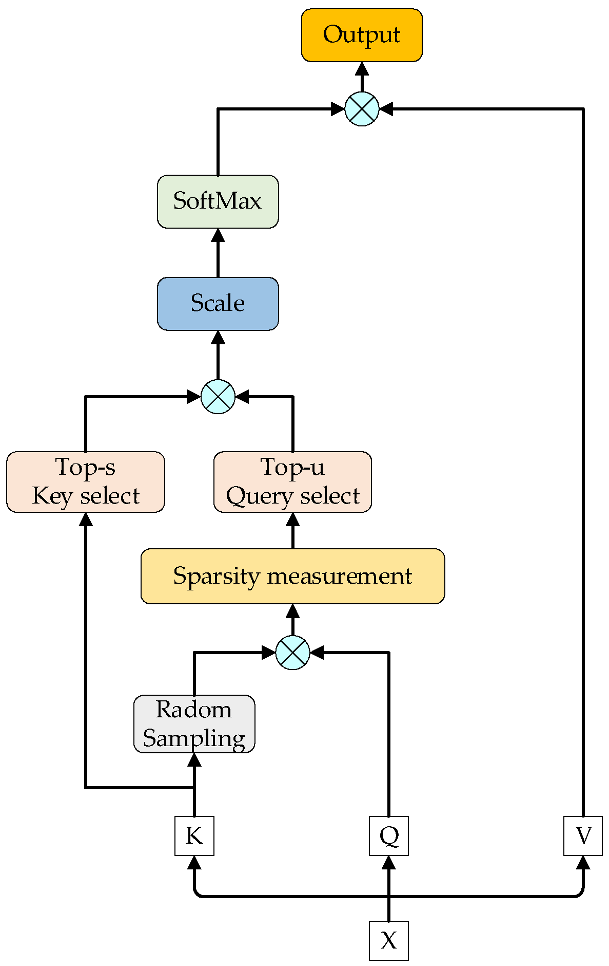
As shown in Figure 2, ProSparse Self-Attention is one of the key components in the Informer model to sparse self-attention weights, reduce compute and memory overhead, and accommodate the need to handle long sequences. For the input array X , the corresponding Query, Key, and Value vectors can be attained by multiplying various weight matrices, as shown in Equations (7)–(9):
Query   = X W Q  
K e y = X W K
Value   = X W V
where X is the input array, and W Q , W K , and W V are weight matrices for linear transformations. First, a dot product is performed on Q and K to obtain an attention score, calculated by Equation (10), which reflects the correlation between each query and key.
S c o r e = Q K T d
In order to select the important Q , ProSparse Self-Attention calculates the sparsity measurement M ( q i , K ) of q i for the key set K , as shown in Equation (11):
M ( q i , K ) = max j { q i T k j d } 1 L K j = 1 L K { q i T k j d }
where k j is the jth key in K , L K is the number of keys, and M ( q i , K ) is the importance between and key set K , determining the difference between the query and key vectors. According to M ( q i , K ) , T o p u queries with greater sparsity are selected, where u is the default value representing the number of query vectors to be retained. Accordingly, important query vectors a high correlation to key set K can be screened. For the selected important query vector, the Softmax operation is performed on the dot product score matrix to convert the attention score into a probability distribution, as described by Equation (12).
AttentionWeights ( q i , K ) = Softmax ( Score ( q i , K ) )
In order to reduce the computation and memory overhead, ProSparse Self-Attention can further sparse the attention weight. For each query vector, only T o p s key vectors with greater attention weights are reserved, where s is the default value representing the number of key vectors to retain. Finally, the sparse attention weight is multiplied by the Value vector, and its summation is employed to obtain the output of ProSparse Self-Attention, as shown in Equation (13).
  Output   ( Q , K , V ) = i = 1 u j = 1 s   AttentionWeights   ( q i , k i j ) v i j
where k i j represents the jth reserved key vector of the ith query vector, and v i j represents the value vector corresponding to k i j . Through the above steps, ProSparse Self-Attention realizes the sparseness and selection of attention weights, reduces the calculation and memory overhead, and retains the key information with a high correlation to the query.

2.2.2. Distilling Layer

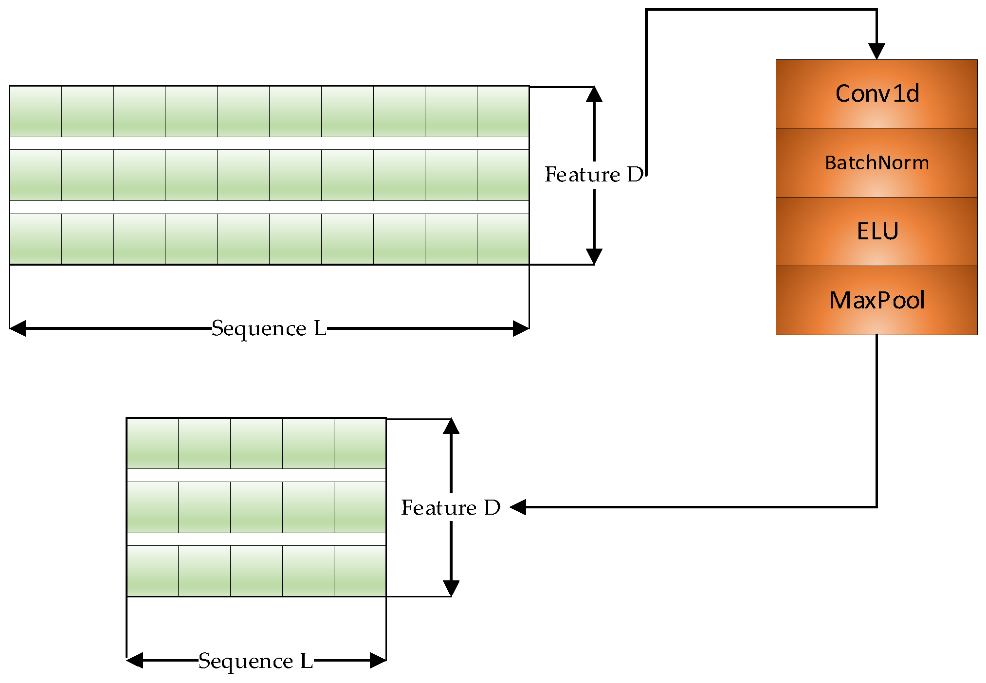
Figure 3 shows the distilling process. For a too-long input sequence, Probsparse Attention only selects T o p u Query for dot product to form dot product pairs, while the rest of the dot product pairs are set as zero. Therefore, many information items are generated when multiplied by Value. In order to alleviate the information redundancy, a distilling layer is located at the end of the encoder [23], which can highlight the essential features, reduce the long sequences’ input complexity, and improve the model’s performance [24]. The “distilling” process is advanced from layer j to layer (j + 1) by Equation (14), where [ ] A B is the attention block.
X j + 1 t = MaxPool ( ELU ( Conv 1 d [ X j t ] A B ) ) )

2.3. BiLSTM Network

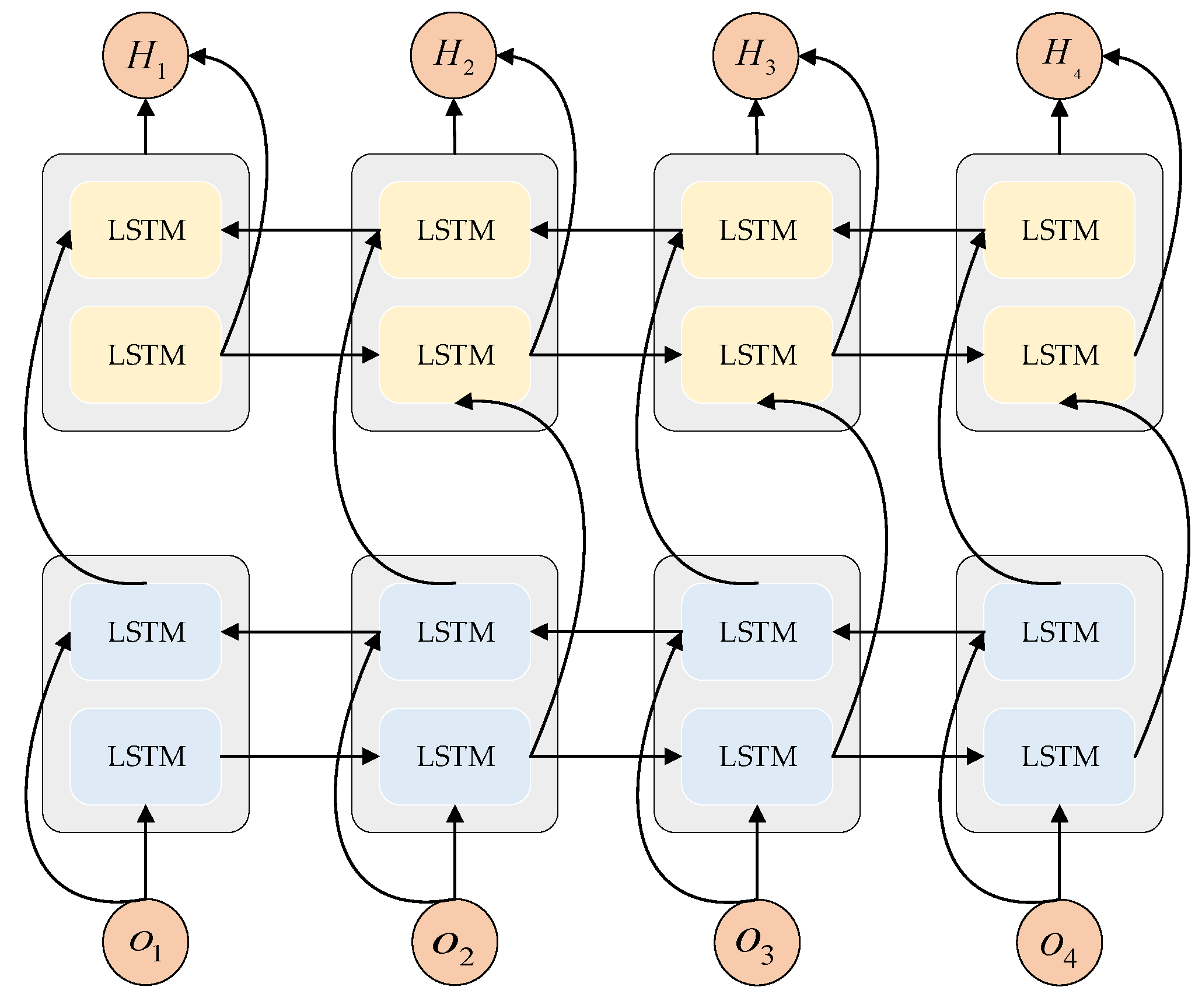
BiLSTM is a variant of recurrent neural networks extensively utilized in time series data processing [25]. As displayed in Figure 4, compared with traditional one-way LSTM, BiLSTM captures more comprehensive contextual information and timing patterns by running two LSTM layers in both forward and backward orientations on the time series [26].
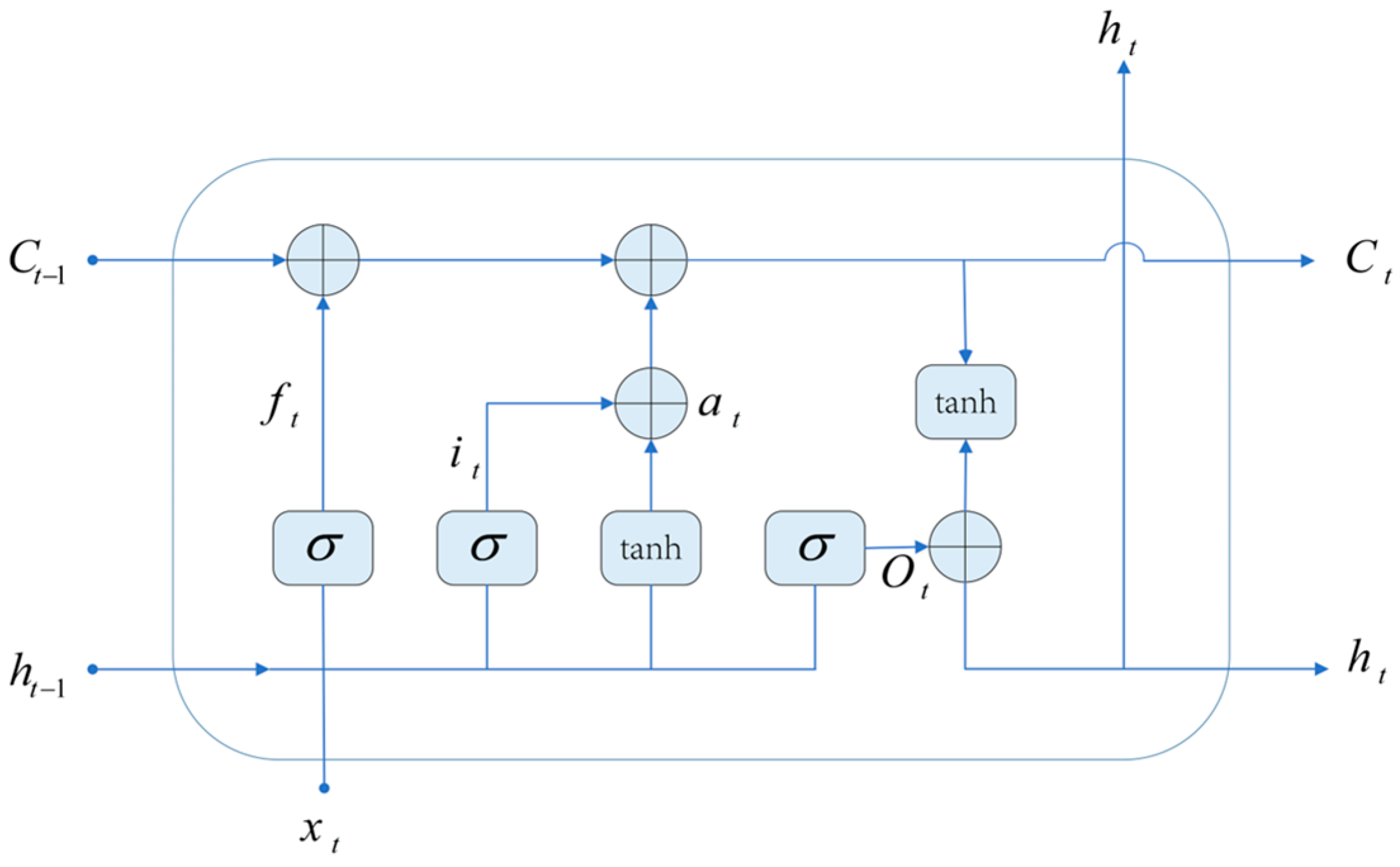
As illustrated in Figure 5, the LSTM unit is the core component of BiLSTM. The main property of LSTM is to introduce gating mechanisms, including input, forget, and output gates, as well as a cell state, to better control the information flow. The forgetting gate indicates the novel information discarded from the cell state, and the calculation formula is presented in Equation (15). The input gate determines the novel information updated into the cell state, and the calculation formula is presented in Equation (16). The cell states first discard some information through the forgetting gate, and then add new candidate information through the input gate. The computation formulas are described by Equations (17) and (18). The output gate indicates the information the next hidden state should contain, and the calculation formula is shown by Equations (19) and (20).
f t = σ ( W f [ x t , h t 1 ] + b f )
i t = σ ( W i [ h t 1 , x t ] + b i )
C ˜ t = tanh ( W C [ h t 1 , x t ] + b C )
C t = f t C t 1 + i t C ˜ t
o t = σ ( W o [ h t 1 , x t ] + b o )
h t = o t tanh ( C t )

3. Proposed Methods

3.1. Frame

This study utilizes the combination of 1D-CNN, Informer encoder, and BiLSTM for TWM. Figure 6 presents the CIEBM tool wear state monitoring algorithm. First, the raw sensor data for tool wear condition monitoring is collected, and the data is pre-processed, including denoising, normalization, and data segmentation. The 1D-CNN neural network is introduced as the basic model for extracting the tool wear state characteristics [27]. CNN can extract local patterns and feature representations related to tool wear from raw sensor data. The Informer encoder is introduced to capture long-term dependencies and global context information in tool wear states. Informer encoders employ self-attention mechanisms to model dependencies between locations in a sequence. Accordingly, features can be correlated from different locations, and important patterns and relationships in the sequence can be captured. The feature sequence extracted by CNN is input into the Informer encoder to obtain a richer feature representation. BiLSTM is introduced to further capture context information in time series data. The Informer encoder’s output sequence is taken as the BiLSTM input, and the relationship between sequence timing and different tool wear states is further extracted through the BiLSTM layer.

3.2. Parameter Settings

The model’s structural parameters are presented in Table 1.

4. Experiments

4.1. Experimental Sets

The current field of tool wear prediction has largely been experimentally validated using the IEEE PHM2010 Challenge dataset. The current work utilized the IEEE PHM2010 [28] challenge dataset as experimental data to evaluate the precision of the CIEBM model.
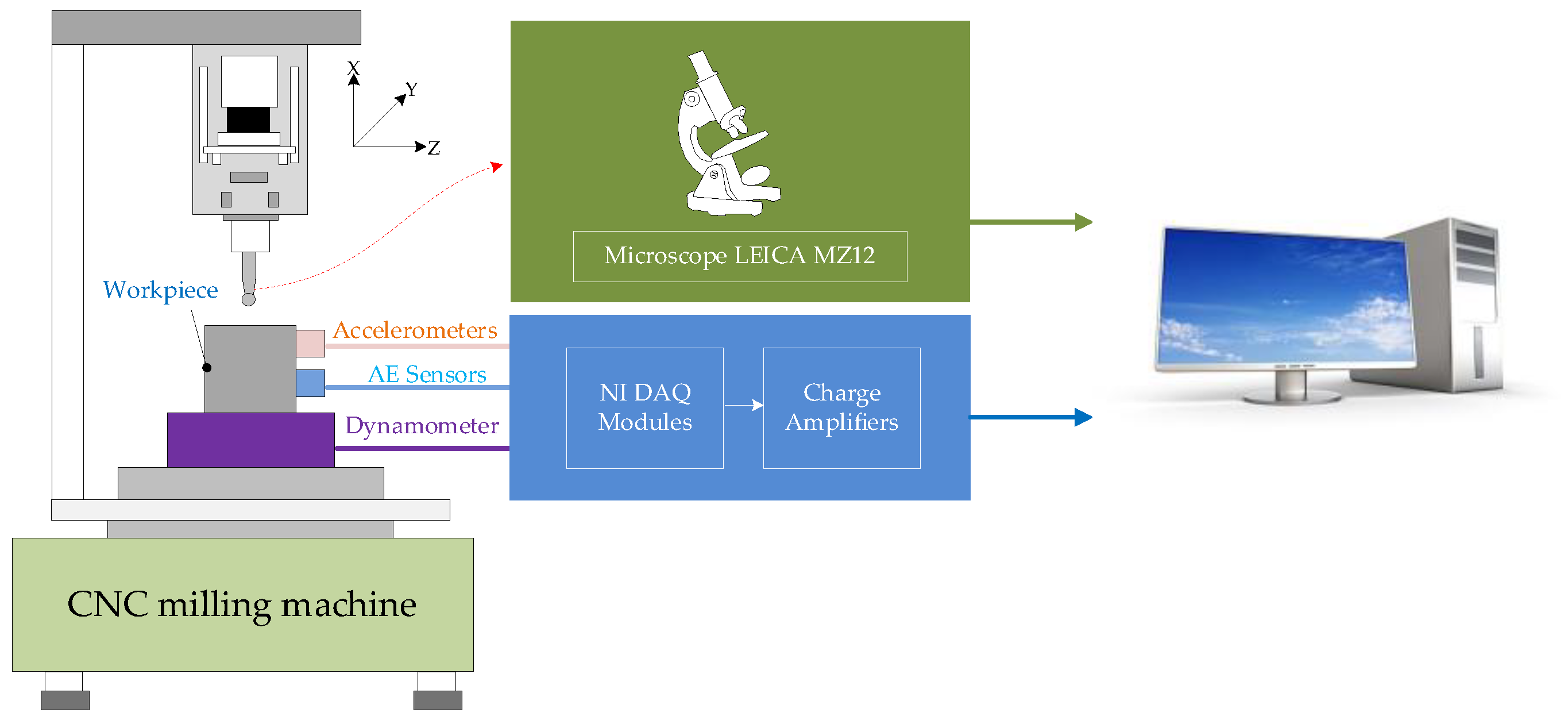
The workpiece is first cut out of the raw material, and the surface of the workpiece is treated by face milling to remove the rough surface containing hard particles. A Kistler cutting force sensor, three-way vibration sensor, and acoustic emission sensor are adopted to acquire cutting force, vibration, and noise signals, respectively [29], as shown in Figure 7. The output of these sensors outputs the corresponding voltage signal through the charge amplifier, which is collected by the NI DAQ PCI 1200 board at a frequency of 50KHz. Acquisition of 7 signals (force_x(N), force_y(N), force_z(N), vibration_x(g), vibration_y(g), vibration_z(g), AE_RMS(v)) is carded. Under dry cutting situations, the surface of the stainless-steel workpiece is machined along the Z-axis with a 3-slot alloy milling cutter. Table 2 presents the specific processing parameters. Experiments were performed with three tools (C1, C4, and C6), and 315 experiments were accomplished on each tool. After each experiment, a microscope measured the tool wear.

4.2. Data Pre-Processing

Since the experimental process includes feeding and retracting processes, the original signal acquired by the sensor contains some invalid data [30]. Meanwhile, a single time step contains less effective information because the original signal has a high sampling rate. In order to better analyze and monitor the tool wear state, it is necessary to conduct data pre-processing [31]. The data pre-processing comprises the following stages:
Invalid data elimination. Since the cutting process includes feeding and retracting processes, 0.5-s data at the beginning and end should be eliminated to avoid the impact of invalid data on the experiment.
Data segmentation. Since the original data contains less effective information in a single time step, the sensor data of each channel in the original data is divided into five segments on average, and the mean value of each segment is extracted to form a new time series.
Data standardization. Data normalization is performed and transformed through Equation (21) to ensure that the numerical ranges of different features are similar and avoid the excessive influence of specific features on model training.
X scalled   = X μ σ
Dataset division. As presented in Table 3, the tool wear state is categorized into light, moderate, and heavy wear, and one-hot coding is employed to perform the label conversion of the three wear states. The different stages of tool wear are shown in Figure 8. The dataset is divided into training, validation, and test sets. The cross-validation method is adopted for verification. Two datasets are selected from the three for training, and the remaining ones are utilized for verification and evaluation. The ratio of the training dataset to the validation dataset was 9:1. Table 4 records the number of category samples included in c1, c4, and c6.

4.3. Hyperparameter Setting

Hyperparameters immediately influence the model’s performance and generalization capability. Different hyperparameter values may result in different complexity and robustness of the model. Hyperparameter selection and optimization is an iterative and experimental process. In this paper, we have tried different combinations of parameters and performed several experiments to finally find the appropriate hyperparameters for the task of tool wear condition monitoring. The best combination of hyperparameters can be found through hyperparameter settings to optimize model performance and improve its generalization ability on new data. Table 5 describes the CIEBM model’s hyperparameter settings.

4.4. Results

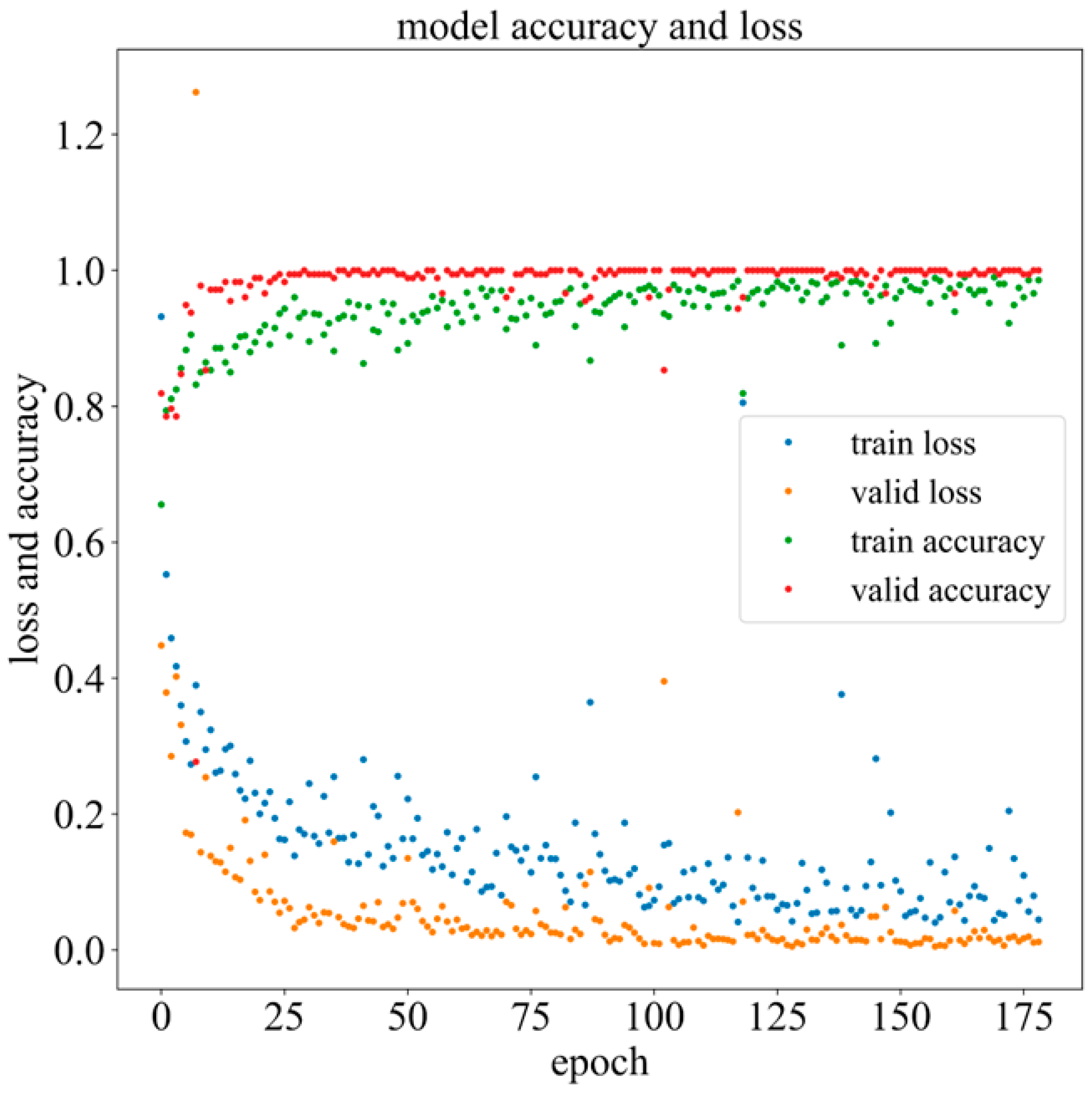
In order to better evaluate the performance of the model, we chose Confusion Matrix, Accuracy, Precision, and Recall to evaluate its performance. The calculations are provided in Equations (22)–(24). As presented in Figure 9, the accuracy of the CIEBM model in dataset identification reaches 99.11% after hyperparameter optimization. The analysis results indicate that the CIEBM model can efficiently detect different wear states of the tool despite the complicated interaction between the tool and the workpiece in the milling process, demonstrating that the CIEBM model has good performance in state recognition.
Accuracy = T P + T N T P + T N + F P + F N
Precision = T P T P + F P
Recall = T P T P + F N
TP: positive samples are classified as positive samples; FP: negative samples are classified as positive samples; TN: negative samples are classified as negative samples; FN: positive samples are classified as negative samples.
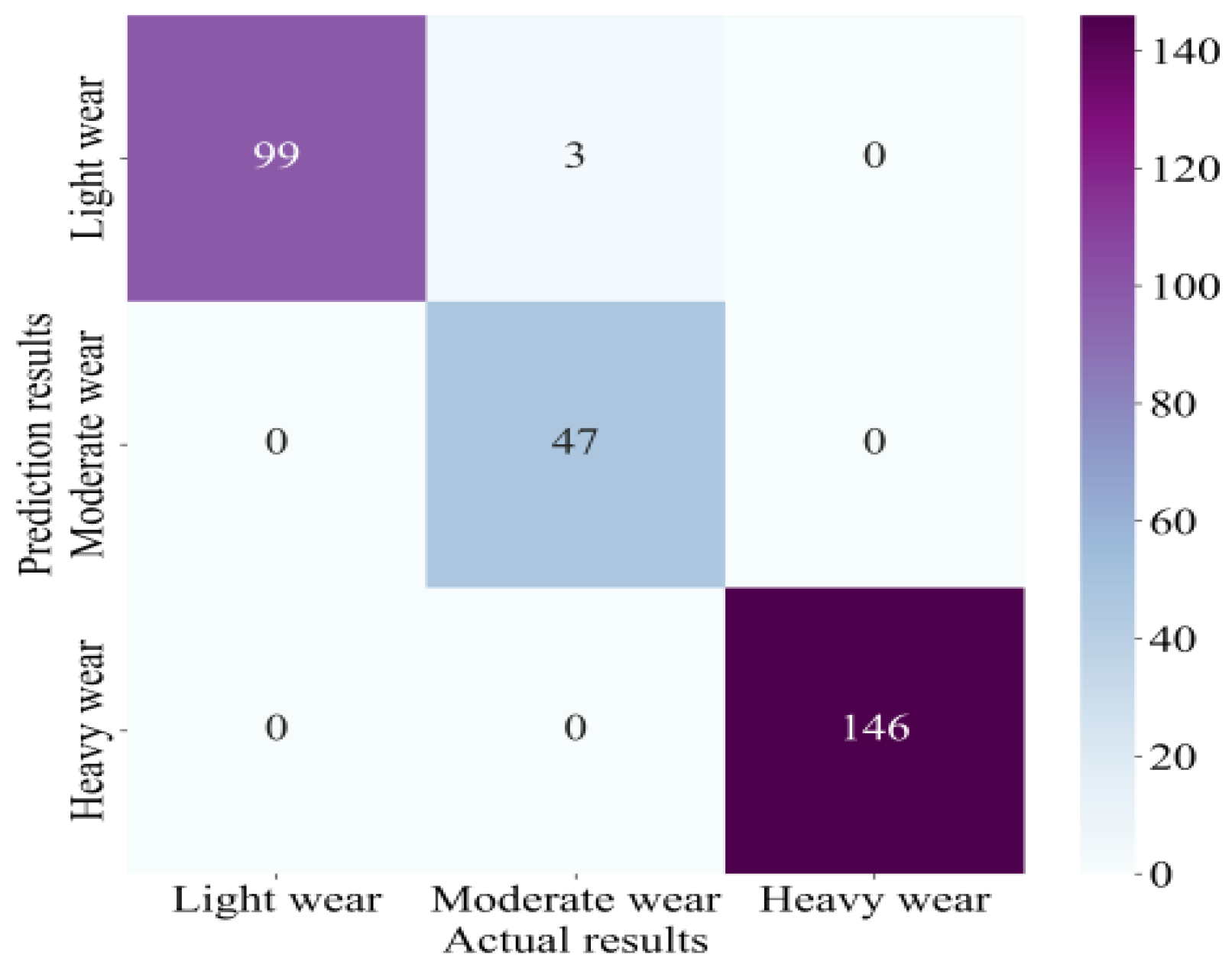
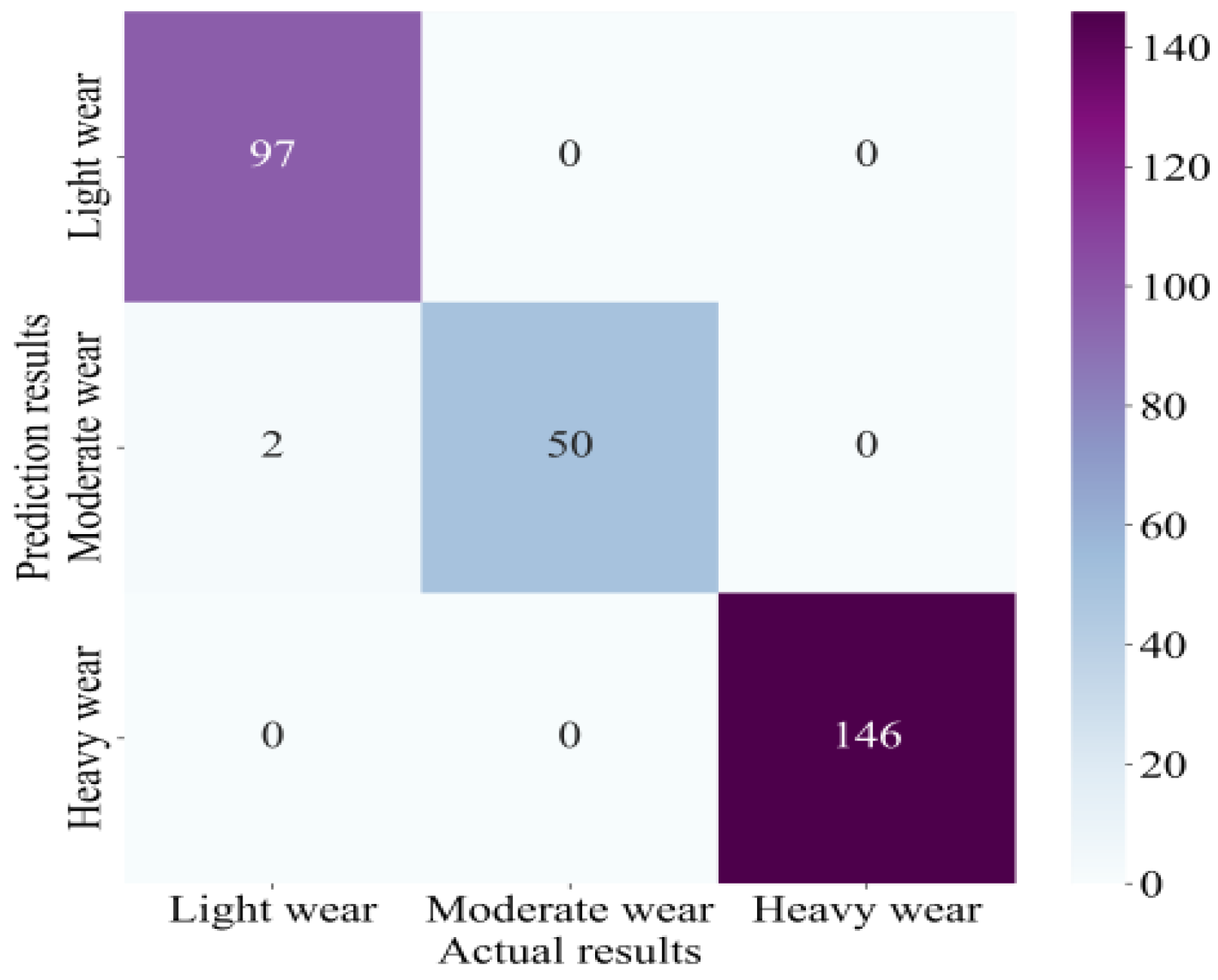
In order to verify the model’s precision under different tool datasets, a confusion matrix is utilized to display the classification results. Taking C1 as an example, its confusion matrix is shown in Figure 10. Its horizontal and vertical coordinates are the true and predicted values, respectively. There are four sample classification errors, among which two samples that originally belonged to light wear were wrongly classified as normal wear, one sample that originally belonged to normal wear was wrongly classified as light wear, and one sample that originally belonged to heavy wear was wrongly classified as light wear. As shown in Figure 11 and Figure 12, there are only one and three classification errors in the C4 and C6 datasets, respectively. Light wear has a precision rate of 100% and a recall rate of 97.05%. Moderate wear has a precision rate of 100% and a recall rate of 94%. Heavy wear has a precision rate of 100% and a recall rate of 100%. These metrics show the excellent performance of the CIEBM model. The established model can efficiently extract the features of different tool wear stages and identify and classify the tool wear state.
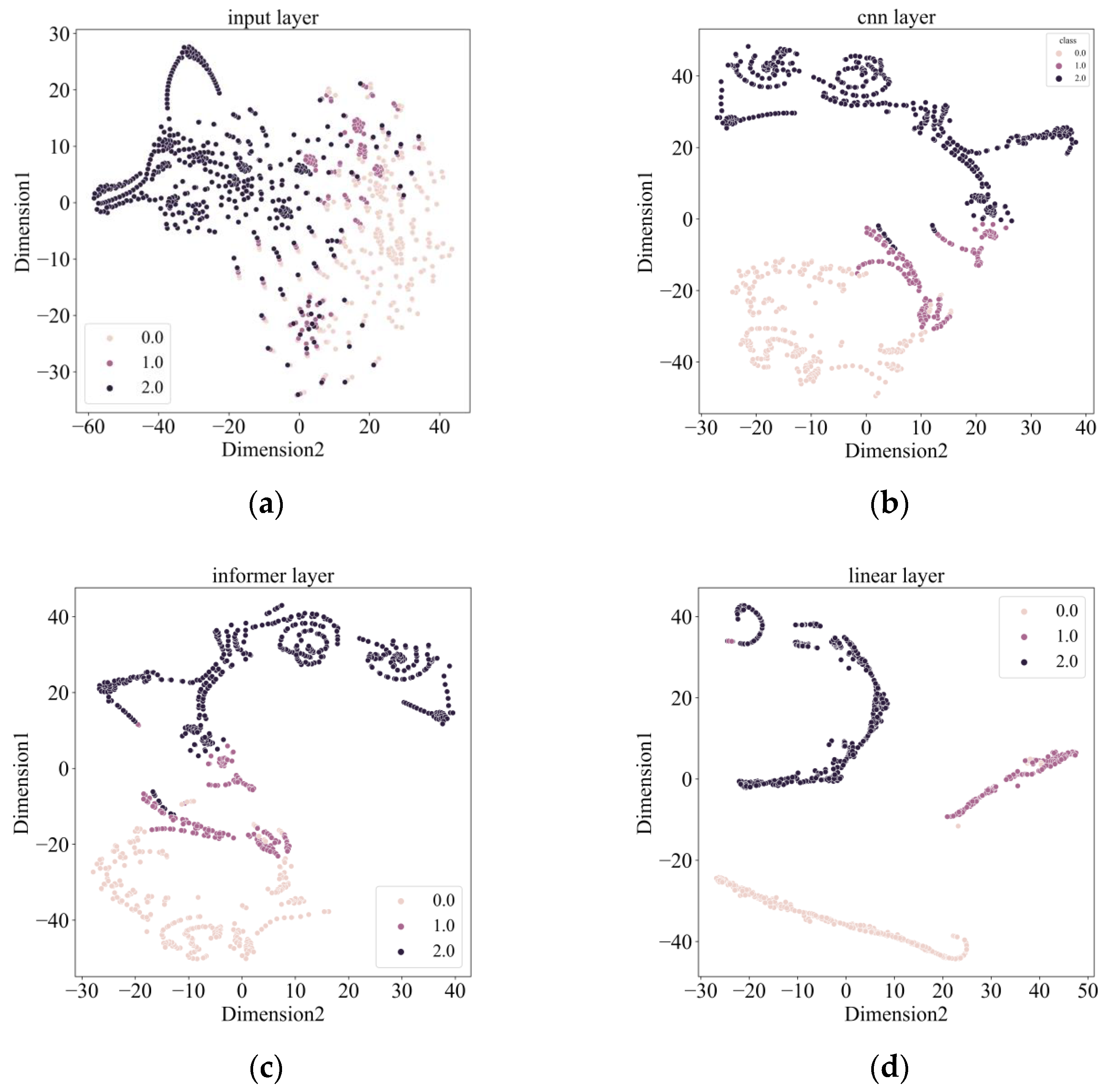
In order to more intuitively observe each network layer’s feature extraction process and demonstrate the ability of the CIEBM model to extract the sensitive features for subsequent state detection effectively, the t-SNE algorithm is utilized for dimension reduction visualization of each network layer, as presented in Figure 13. Figure 13a describes the t-SNE visualization results of the original signal with mixed data and a poor clustering effect. Figure 13b describes the t-SNE visualization results of the CNN layer. The first-type samples have been separated, and there is an aggregation trend among the same type of samples. Figure 13c shows the t-SNE visualization results through the Informer layer. Except for some mixed samples, all samples were classified, and the three types of samples were completely separated. Figure 13d shows the t-SNE visualization results of the Linear layer. All samples are classified, and the clustering effect is obvious. It can be seen that the CIEBM model can effectively identify and classify different tool wear states.

4.5. Comparative Analysis

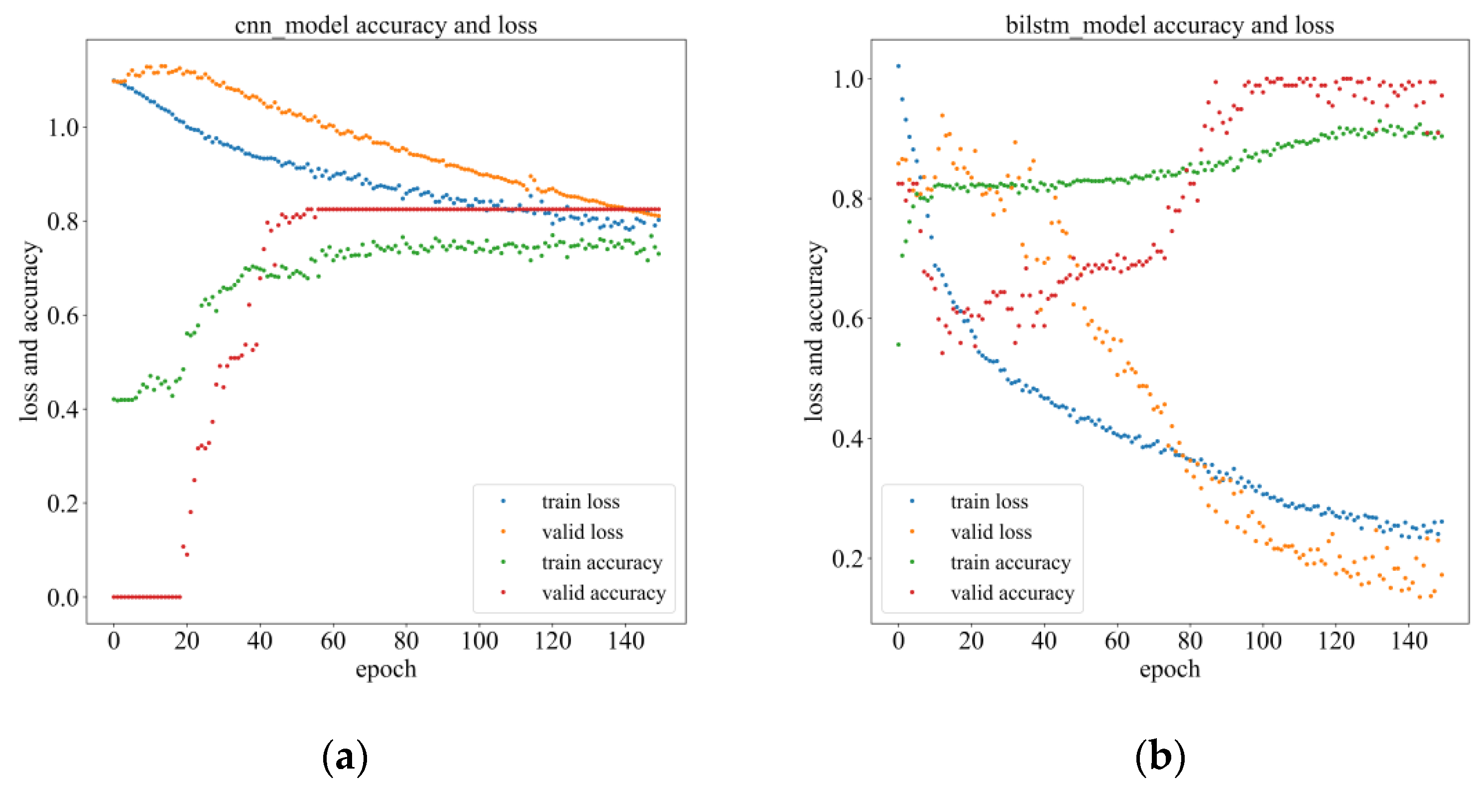
In order to evaluate the advantages of the established CIEBM model, it is compared with the CNN and BiLSTM models in the PHM2010 dataset with the same hyperparameter settings. As shown in Figure 14a,b, the accuracy of the CIEBM model is increased by 17.42% and 2.05% compared with CNN and BiLSTM, respectively. Comparing the convergence rates of different models indicates that the CIEBM model has the maximum convergence rate, indicating that it can extract valuable features from the input data to represent the key information in the data. At the same time, the CIEBM model can learn and adapt the relationship between the features extracted from the training data and the tool wear faster.
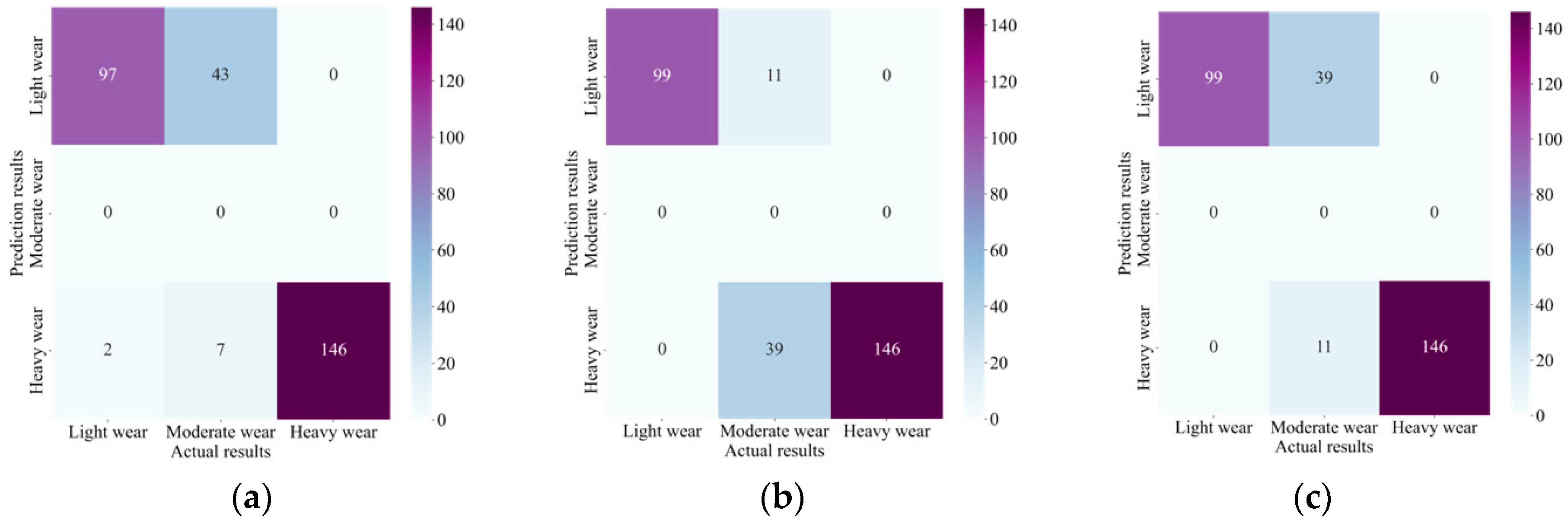
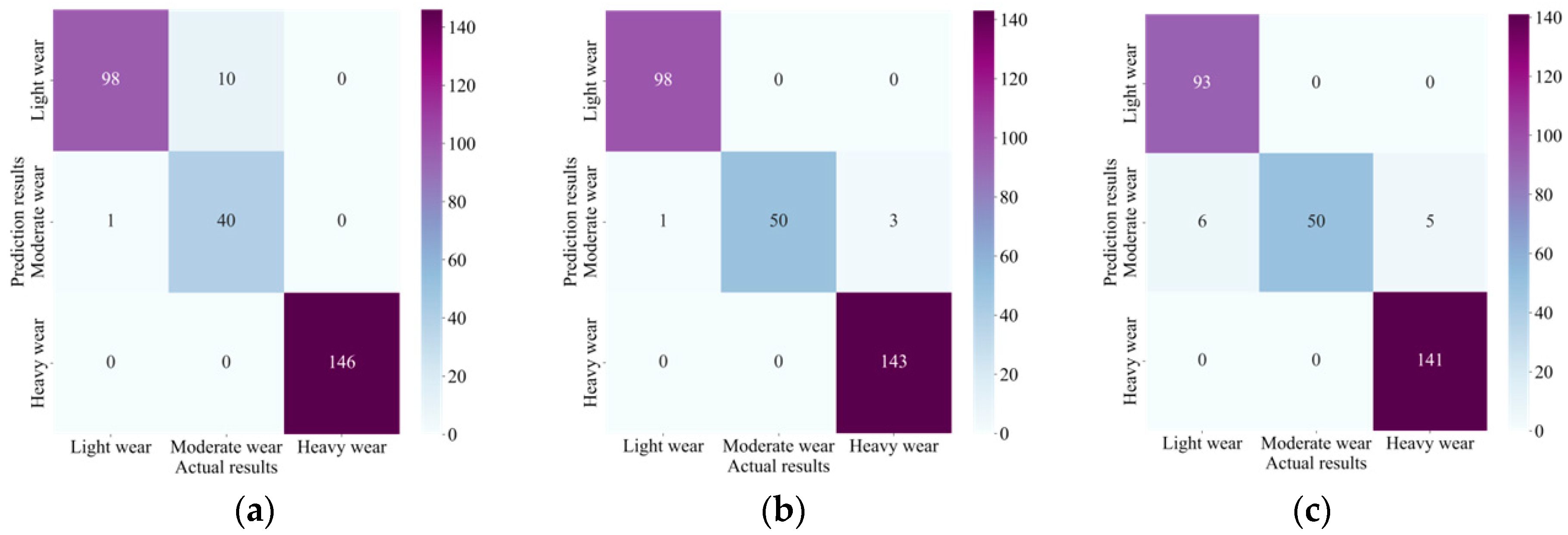
For a more intuitive comparative analysis, Figure 15 and Figure 16 present the confusion matrix of the prediction results of these models. Through the experiment, it can be found that the identification precision of each model in the light and heavy wear is generally higher than that in the moderate wear due to the faster wear change rate of the early wear and heavy wear. As presented in Figure 14, the CNN model is completely wrong in the moderate wear stage with a slower change rate because the CNN is mainly concerned with local patterns and features, and there may be important correlations between each time step in time series data. However, the traditional 1D-CNN mainly focuses on feature extraction from local neighborhoods and cannot utilize global context information. Additionally, underfitting occurs when using only the CNN model due to the lack of feature representation. As presented in Figure 15, the BiLSTM model performs well in time series and can capture long-term dependence. However, it lacks the ability to use global modeling in tool wear time series, considerably increasing the misclassification in the prediction of moderate and heavy wear, especially in the moderate wear stage. This demonstrates the effectiveness of the CIEBM model with the Informer encoder module for global feature modeling.
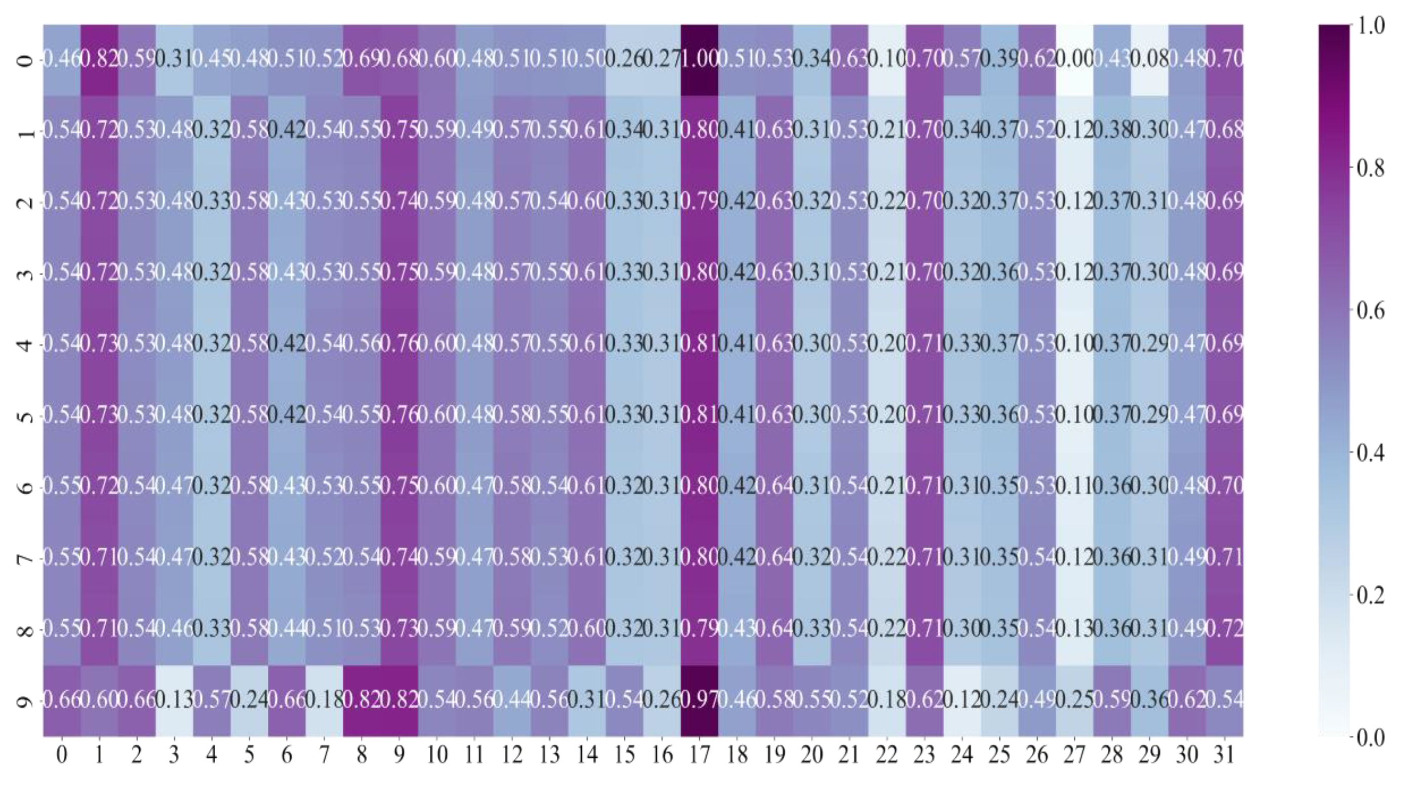
As shown in Figure 17, attention mechanism links are visualized to form attention heat maps to further illustrate the Informer encoder’s role, which can understand the key features that the model relies on when making classifications. As revealed from the attention heat map, the Informer encoder can make the CIEBM model better focus on features that are more closely dependent on the tool wear condition monitoring and improve the model’s computational performance through the sparse attention mechanism, demonstrating the effectiveness of the introduction of the Informer encoder module.

5. Conclusions

A tool wear state monitoring approach using CNN, Informer encoder, and BiLSTM was proposed to evaluate its performance on the tool wear state dataset. The experimental results and analysis demonstrate the following results:
(1)
Experimental results reveal that the presented TWM approach based on CNN, Informer encoder, and BiLSTM has high accuracy in TWM. All of them reached over 95% in the relevant evaluation indexes, reflecting the excellent performance of the CIEBM model, which can efficiently classify and forecast the tool wear state.
(2)
In tool wear monitoring, CNN can extract spatial features from sensor data. Informer encoders can model long-term dependencies and capture global context information with ProbSparse Self-Attention and a feedforward neural network layer. BiLSTM captures temporal patterns and context information to further improve monitoring accuracy.
(3)
Our model is the first to use CNN, an Informer encoder, and BiLSTM together for tool wear condition monitoring, and it is also the first to target global feature modeling based on the non-linearity of the tool wear process to enable the model to better learn the relationship between the features of different wear stages. This is of great importance for further research.
(4)
Further analysis shows that our method has an excellent classification impact on normal and different degrees of wear, and the confusion between normal and heavy wear is slight, indicating that the method can effectively distinguish tool states with different degrees of wear.
In summary, the tool wear state monitoring approach using CNN, Informer encoder, and BiLSTM performed well in the experiment. This method has significant application value for TWM in the industrial field. Nevertheless, many details still need to be improved, such as further optimization of the model architecture, hyperparameter adjustment, and dataset size expansion, to enhance the monitoring’s precision and robustness.
In future work, the method of combining physical models of tool wear with deep learning will be further investigated. By modeling the physical model, the interpretability of deep learning will be further improved while providing a theoretical basis for optimizing the deep learning network model for the production scenario of tool wear. In the next phase, we will continue to conduct field experiments to study wear under variable working conditions to further improve the generalization ability of the model.

Author Contributions

This article has the help of all the authors. X.X. provided initial ideas and defined research objectives, designed experiments and selected appropriate algorithms, developed codes for the BiLSTM model and performed initial tests, verified experimental results, guaranteed the accuracy of experimental results, and wrote the first draft of the manuscript. W.S. collected, cleaned, and organized the dataset used in the study. Reviewed and edited the manuscript, improving its clarity and coherence. Y.L. (Yingming Li) and Y.L. (Yue Liu) reviewed and edited the manuscript, improving its clarity and coherence. M.H. oversaw the research project, providing guidance and feedback. Secured funding for the research. All authors have read and agreed to the published version of the manuscript.

Funding

The research was funded by the Ministry of Industry and Information Technology’s High-end Numerical Control Systems and Servo Motors Project (Grant No. ZTZB-22-009-001).

Data Availability Statement

All data are contained within the article.

Conflicts of Interest

The authors declare no conflict of interest.

Nomenclature

y [ t ] Calculated output
bShift factor
w [ i ] Weighting coefficient
x [ ] Sequence input value
f ( x ) Activation function output
W Weight matrix
X Model input
Q/qQuery vector
K/kKey vector
V/vValue vector
L Number of vectors
dLength of vector
M ( ) Attention score
f t Forget gate output
C t 1 Previous cell state
i t Input gate output
C ˜ t Candidate
C t New cell state
o t Output gate output
h t Hidden state
TPTrue positive
FNFalse negative
FPFalse positive
TNTrue negative

References

  1. Zhang, C.; Wang, W.; Li, H. Tool wear prediction method based on symmetrized dot pattern and multi-covariance Gaussian process regression. Measurement 2022, 189, 110466. [Google Scholar] [CrossRef]
  2. Shi, D.; Gindy, N.N. Tool wear predictive model based on least squares support vector machines. Mech. Syst. Signal Process 2007, 21, 1799–1814. [Google Scholar] [CrossRef]
  3. Gomes, M.C.; Brito, L.C.; da Silva, M.B.; Duarte, M.A.V. Tool wear monitoring in micromilling using Support Vector Machine with vibration and sound sensors. Precis. Eng. 2021, 67, 137–151. [Google Scholar] [CrossRef]
  4. Cheng, Y.; Gai, X.; Jin, Y.; Guan, R.; Lu, M.; Ding, Y. A new method based on a WOA-optimized support vector machine to predict the tool wear. Int. J. Adv. Manuf. Technol. 2022, 121, 6439–6452. [Google Scholar] [CrossRef]
  5. Gai, X.; Cheng, Y.; Guan, R.; Jin, Y.; Lu, M. Tool wear state recognition based on WOA-SVM with statistical feature fusion of multi-signal singularity. Int. J. Adv. Manuf. Technol. 2022, 123, 2209–2225. [Google Scholar] [CrossRef]
  6. Xu, D.; Qiu, H.; Gao, L.; Yang, Z.; Wang, D. A novel dual-stream self-attention neural network for remaining useful life estimation of mechanical systems. Reliab. Eng. Syst. Safe 2022, 222, 108444. [Google Scholar] [CrossRef]
  7. Liu, B.; Li, H.; Ou, J.; Wang, Z.; Sun, W. Intelligent recognition of milling tool wear status based on variational auto-encoder and extreme learning machine. Int. J. Adv. Manuf. Technol. 2022, 119, 4109–4123. [Google Scholar] [CrossRef]
  8. Liu, Z.; Hao, K.; Geng, X.; Zou, Z.; Shi, Z. Dual-Branched Spatio-Temporal Fusion Network for Multihorizon Tropical Cyclone Track Forecast. IEEE J. Sel. Top. Appl. Earth Obs. Remote Sens. 2022, 15, 3842–3852. [Google Scholar] [CrossRef]
  9. Dai, W.; Liang, K.; Wang, B. State Monitoring Method for Tool Wear in Aerospace Manufacturing Processes Based on a Convolutional Neural Network (CNN). Aerospace 2021, 8, 335. [Google Scholar] [CrossRef]
  10. García-Pérez, A.; Ziegenbein, A.; Schmidt, E.; Shamsafar, F.; Fernández-Valdivielso, A.; Llorente-Rodríguez, R.; Weigold, M. CNN-based in situ tool wear detection: A study on model training and data augmentation in turning inserts. J. Manuf. Syst. 2023, 68, 85–98. [Google Scholar] [CrossRef]
  11. Kothuru, A.; Nooka, S.P.; Liu, R. Application of deep visualization in CNN-based tool condition monitoring for end milling. Procedia Manuf. 2019, 34, 995–1004. [Google Scholar] [CrossRef]
  12. Wu, X.; Liu, Y.; Zhou, X.; Mou, A. Automatic Identification of Tool Wear Based on Convolutional Neural Network in Face Milling Process. Sensors 2019, 19, 3817. [Google Scholar] [CrossRef] [PubMed]
  13. Qin, X.; Zhang, W.; Gao, S.; He, X.; Lu, J. Sensor Fault Diagnosis of Autonomous Underwater Vehicle Based on LSTM. In Proceedings of the 2018 37th Chinese Control Conference (CCC), Wuhan, China, 25–27 July 2018; pp. 6067–6072. [Google Scholar] [CrossRef]
  14. Xu, W.; Miao, H.; Zhao, Z.; Liu, J.; Sun, C.; Yan, R. Multi-Scale Convolutional Gated Recurrent Unit Networks for Tool Wear Prediction in Smart Manufacturing. Chin. J. Mech. Eng. 2021, 34, 53. [Google Scholar] [CrossRef]
  15. Liu, X.; Zhang, B.; Li, X.; Liu, S.; Yue, C.; Liang, S.Y. An approach for tool wear prediction using customized DenseNet and GRU integrated model based on multi-sensor feature fusion. J. Intell. Manuf. 2023, 34, 885–902. [Google Scholar] [CrossRef]
  16. Cheng, M.; Jiao, L.; Yan, P.; Jiang, H.; Wang, R.; Qiu, T.; Wang, X. Intelligent tool wear monitoring and multi-step prediction based on deep learning model. J. Manuf. Syst. 2022, 62, 286–300. [Google Scholar] [CrossRef]
  17. Liu, H.; Liu, Z.; Jia, W.; Zhang, D.; Wang, Q.; Tan, J. Tool wear estimation using a CNN-transformer model with semi-supervised learning. Meas. Sci. Technol. 2021, 32, 125010. [Google Scholar] [CrossRef]
  18. Liu, H.; Liu, Z.; Jia, W.; Lin, X.; Zhang, S. A novel transformer-based neural network model for tool wear estimation. Meas. Sci. Technol. 2020, 31, 065106. [Google Scholar] [CrossRef]
  19. Lin, H.; Sun, Q. Financial Volatility Forecasting: A Sparse Multi-Head Attention Neural Network. Information 2021, 12, 419. [Google Scholar] [CrossRef]
  20. Zou, R.; Duan, Y.; Wang, Y.; Pang, J.; Liu, F.; Sheikh, S.R. A novel convolutional informer network for deterministic and probabilistic state-of-charge estimation of lithium-ion batteries. J. Energy Storage 2023, 57, 106298. [Google Scholar] [CrossRef]
  21. Vaswani, A.; Shazeer, N.; Parmar, N.; Uszkoreit, J.; Jones, L.; Gomez, A.N.; Kaiser, Ł.; Polosukhin, I. Attention is all you need. Advances in Neural Information Processing Systems 30 (NIPS 2017). In Proceedings of the 31st International Conference on Neural Information Processing Systems, Long Beach, CA, USA, 4–9 December 2017; pp. 6000–6010. [Google Scholar] [CrossRef]
  22. Zhou, H.; Zhang, S.; Peng, J.; Zhang, S.; Zhang, W. In Informer: Beyond efficient transformer for long sequence time-series forecasting. In Proceedings of the AAAI Conference on Artificial Intelligence, Virtual, 2–9 February 2021. [Google Scholar] [CrossRef]
  23. Li, R.; Ye, X.; Yang, F.; Du, K.L. ConvLSTM-Att: An Attention-Based Composite Deep Neural Network for Tool Wear Prediction. Machines 2023, 11, 297. [Google Scholar] [CrossRef]
  24. Xie, X.; Huang, M.; Liu, Y.; An, Q. Intelligent Tool-Wear Prediction Based on Informer Encoder and Bi-Directional Long Short-Term Memory. Machines 2023, 11, 94. [Google Scholar] [CrossRef]
  25. Li, W.; Liang, Y.; Wang, S. Data Driven Smart Manufacturing Technologies and Applications; Springer: Berlin/Heidelberg, Germany, 2021. [Google Scholar] [CrossRef]
  26. Sun, M.; Liu, Z.; Zhang, M.; Liu, Y. Chinese computational linguistics and natural language processing based on naturally annotated big data. In Proceedings of the S14th China National Conference, CCL 2015 and Third International Symposium, NLP-NABD 2015, Guangzhou, China, 13–14 November 2015. [Google Scholar] [CrossRef]
  27. Cheng, Y.; Gai, X.; Guan, R.; Jin, Y.; Lu, M.; Ding, Y. Tool wear intelligent monitoring techniques in cutting: A review. J. Mech. Sci. Technol. 2023, 37, 289–303. [Google Scholar] [CrossRef]
  28. 2010 phm Society Conference Data Challenge 2010. Available online: https://phmsociety.org/competition/phm/10 (accessed on 6 September 2023).
  29. Huang, Q.; Wu, D.; Huang, H.; Zhang, Y.; Han, Y. Tool Wear Prediction Based on a Multi-Scale Convolutional Neural Network with Attention Fusion. Information 2022, 13, 504. [Google Scholar] [CrossRef]
  30. Du, M.; Wang, P.; Wang, J.; Cheng, Z.; Wang, S. Intelligent Turning Tool Monitoring with Neural Network Adaptive Learning. Complexity 2019, 2019, 8431784. [Google Scholar] [CrossRef]
  31. Bergs, T.; Holst, C.; Gupta, P.; Augspurger, T. Digital image processing with deep learning for automated cutting tool wear detection. Procedia Manuf. 2020, 48, 947–958. [Google Scholar] [CrossRef]
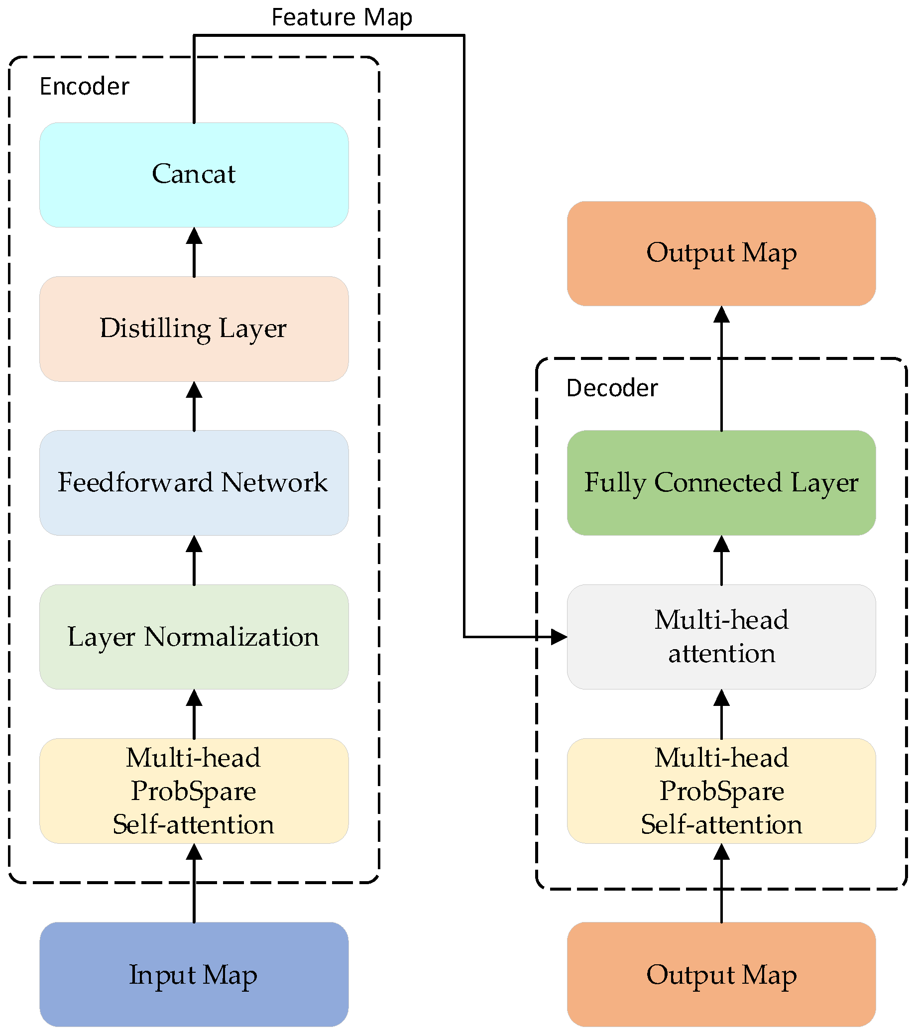
Figure 1. Network structure of the Informer.
Lubricants 11 00389 g001
Figure 2. Network structure of ProSparse Self-Attention.
Lubricants 11 00389 g002
Figure 3. Network structure of the distilling layer.
Lubricants 11 00389 g003
Figure 4. Network structure of BiLSTM.
Lubricants 11 00389 g004
Figure 5. Network structure of LSTM.
Lubricants 11 00389 g005
Figure 6. Network structure of CIEBM.
Lubricants 11 00389 g006
Figure 7. Schematic diagram of the experimental setup.
Lubricants 11 00389 g007
Figure 8. Diagram of different stages of tool wear: (a) light wear; (b) moderate wear; (c) heavy wear.
Lubricants 11 00389 g008
Figure 9. Training loss rate and precision of the CIEBM model.
Lubricants 11 00389 g009
Figure 10. Classification confusion matrix results of the C1 tool wear state.
Lubricants 11 00389 g010
Figure 11. Classification confusion matrix results of the C4 tool wear state.
Lubricants 11 00389 g011
Figure 12. Classification confusion matrix results of the C6 tool wear state.
Lubricants 11 00389 g012
Figure 13. t-SNE visualization results of each network layer of the CIEBM model: (a) Input layer visualization results; (b) CNN layer visualization results; (c) Informer layer visualization results; (d) Linear layer visualization results.
Lubricants 11 00389 g013
Figure 14. (a) CNN model’s loss rate and precision. (b) Loss rate and accuracy of the BiLSTM model.
Lubricants 11 00389 g014
Figure 15. CNN model confusion matrix results of tool wear status classification: (a) C1; (b) C4; (c) C6.
Lubricants 11 00389 g015
Figure 16. BiLSTM model confusion matrix results of tool wear status classification: (a) C1; (b) C4; (c) C6.
Lubricants 11 00389 g016
Figure 17. Attention heat map visualization results of the Informer encoder.
Lubricants 11 00389 g017
Table 1. The CIEBM structural parameters.
LayerOutput Shape
Conv1D(20, 16)
MaxPooling(10, 16)
Informer Encoder(10, 32)
LayerNormalization(10, 32)
Attention(10, 32)
Dropout(10, 32)
Lstm(10, 30)
Dropout(10, 30)
Lstm(10, 15)
Dropout(10, 15)
Lstm(1, 15)
Dropout(1, 15)
Output(1, 3)
Table 2. Experimental test parameters.
ParameterValue
Spindle10,400 (r/min)
Feed rate1555 (mm/min)
Depth of cut (y direction, radial)0.125 (mm)
Depth of cut (z direction, axial)0.2 (mm)
Sampling rate50 (kHz)
Workpiece materialStainless steel (HRC52)
Table 3. Classification standard for tool wear conditions.
Degree of WearLight WearModerate WearHeavy Wear
Wear loss (mm)0–0.120.12–0.170.17–0.30
One-hot coding012
Table 4. Number of different types of samples contained in each state.
Tool NumberCategory
Light WearModerate WearHeavy Wear
C19950146
C49950146
C69950146
Table 5. Hyperparameter settings of the CIEBM model.
ProjectValue
Epoch150
Batch size32
Learning rate0.0001
Dropout0.2
Objective functionCrossEntropy Loss
Objective functionRMSprop
Activation functionReLU
Bilstm Stack number3
Disclaimer/Publisher’s Note: The statements, opinions and data contained in all publications are solely those of the individual author(s) and contributor(s) and not of MDPI and/or the editor(s). MDPI and/or the editor(s) disclaim responsibility for any injury to people or property resulting from any ideas, methods, instructions or products referred to in the content.