Application of Machine Learning Models to the Analysis of Skid Resistance Data

Abstract

This paper evaluates the ability of some state-of-the-art Machine Learning models, namely SVM (support vector machines), DT (decision tree) and MLR (multiple linear regression), to predict pavement skid resistance. The study encompasses both regression and classification tasks. In the regression task, the aim is to predict the coefficient of friction values, while the classification task seeks to identify three classes of skid resistance: good, intermediate and bad. The dataset used in this work was gathered through an extensive test campaign that involved a fifth-wheel device to measure the coefficient of friction at different slip ratios on different road surfaces, vehicle speeds, tire tread depths and water depths. It was found that the RBF-SVM model, due to its ability to capture non-linear relationships between the features and the target for a relatively small dataset, is the most adapted tool compared with, on one side, MLR, linear SVM and DT models for the regression task and, on the other side, linear SVM and DT models for the classification task. The paper also discusses the strengths and weaknesses of the investigated models based on the underlying physical phenomena related to skid resistance.

1. Introduction

Road safety heavily relies on the skid resistance of road surfaces, as it plays a crucial role in vehicle stability and braking performance [1,2,3]. In order to ensure user safety and vehicle dynamic stability, technical solutions commonly referred to as advanced driver assistance systems (ADAS) have emerged in recent years [4,5,6]. Using data from various sensors and advanced algorithms, these systems interpret the vehicle’s surrounding environment to alert the driver or to take control of the vehicle in order to mitigate potential hazards. While ADAS technologies based on object detection (vehicle, pedestrian, traffic signs, and others) have been extensively studied [7,8,9,10], the specific area concerning the interaction between the vehicle and road surface has received less interest. Among the reasons that might explain this observation, the following two points can be highlighted:

• The complexity and variability associated with skid resistance prediction, which involves multiple factors, such as vehicle dynamics, environmental conditions, road surface characteristics, and tire characteristics [11].
• The availability of direct skid resistance sensors, which usually include tire mounted systems [12]. The integration of such devices is unviable for commercial vehicles.

The absence of skid resistance consideration in the development of ADAS makes these technologies incomplete solutions, particularly in degraded conditions (adverse weather, presence of contaminants, etc.). Indeed, skid resistance, which represents the contribution of road surfaces to tire/road friction, allows drivers to control their vehicles. A low skid resistance can induce accidents (lane departure, collisions). Predicting skid resistance may contribute significantly to enhancing road users’ safety and optimize maintenance operations (that would, in turn, mitigate turn environmental impacts).

The literature commonly refers to the following two approaches for modeling pavement skid resistance: (1) analytical models and (2) numerical models [13].

• Analytical models rely on simplified theoretical equations that describe the interaction between the tire and the road surface. One well-known example is the Penn state model, forming the basis of the International Friction Index (IFI), which correlates skid resistance with pavement macro-texture and tire slip speed [14]. Another significant model is the Pacejka “Magic formula” widely used for analyzing the frictional behavior of tire rubber in vehicle engineering [15].
• On the other hand, numerical models [16,17,18] are more sophisticated than analytical techniques. Generally based on finite element solvers, these models can simulate the tire–pavement interaction with great accuracy by considering various factors, such as inflation pressure, tire load, tire tread depth, water depth, slip speed, surface temperature and more.

Although these both approaches are valuable, their practical deployment is still limited due to the difficulty of finding a balance between the consideration of the involved mechanisms and ensuring that the models can operate within a reasonable computational time. A promising alternative to the current methods consists of developing Machine Learning (ML) techniques, in which models are able to learn from data. While research on this topic is still limited, recent studies have demonstrated the potential of ML models to predict skid resistance and its evolution over time [19,20,21,22]. ML involves two main tasks: regression and classification. Previous ML studies on skid resistance have predominantly focused on regression. Nevertheless, a classification approach, such as labeling road surfaces as “good” or “bad,” would be more beneficial for non-expert users, including road authorities and drivers.

The aim of this work is to evaluate the ability of some state-of-the-art ML models to predict pavement skid resistance through regression and classification studies. As shown in Figure 1, the investigated models take as inputs the influencing factors and provide as outputs the tire/road coefficient of friction or classes of skid resistance. In this study, the influencing factors were selected based on their significant effect on skid resistance and available data: the vehicle speed (as part of the vehicle dynamics), the water depth (as part of environmental conditions), the road surface macrotexture (as part of the pavement characteristics) and the tire tread depth (as part of the tire characteristics).

Three models were examined in this study: (1) multiple linear regression, (2) support vector machines and (3) decision trees. The selection of these models was guided by the following criteria:

• Considering the size of the dataset (Section 3), we prioritized simpler models over complex ones (such as neural networks, random forests, etc.). Complex models, characterized by a large set of parameters, tend to be more prone to overfitting [23], especially when dealing with a relatively small dataset.
• Model interpretability: The SVM algorithm, as the following section will illustrate, is based on a solid theoretical foundation. On the other hand, the DT is more easily interpretable for non-experts.
• The necessity to evaluate both non-linear and linear models.

In the next section, the theory of the models studied is presented. A description of the database is also given. The results are then presented and discussed.

2. Algorithm Description

2.1. Multiple Linear Regression

Multiple linear regression (MLR) can be seen as a generalization of a simple linear regression model in order to address problems with multiple independent variables. It assumes that the relationship between the input’s features $X=\left\{X_0,X_1,\dots ,X_p\right\}$ and the predicted value $Y$ can be approximated by a linear equation, as shown by Equation (1).

$$Y={\beta }_0+{\beta }_1.X_1+{\beta }_2.X_2+\dots +{\beta }_p.X_p+\epsilon ,$$

(1)

where

• $\beta =\left\{{\beta }_0, {\beta }_1, \dots , {\beta }_p\right\}$ are unknown constants representing the model parameters;
• $\epsilon$ is the model error;
• ${\beta }_j$ quantifies the association (weights) between the variable $X_j$ and the desired response $Y$. Thus, ${\beta }_j$ can be seen as the average effect on Y of a one-unit increase in $X_j$, holding all other features fixed.

Different methods can be used to estimate the model parameters $\left(\beta \right)$ using a training dataset. The most common approach involves minimizing the least squares criterion, by choosing $\widehat{\beta }=\left\{{\widehat{\beta }}_0, {\widehat{\beta }}_1, \dots , {\widehat{\beta }}_p\right\}$ which minimizes the sum of squared residuals (SSR).

$$SSR={{\displaystyle \sum }}_{i=1}^n{\left(y_i-{\widehat{\beta }}_0-{\widehat{\beta }}_1.x_{i1}-{\widehat{\beta }}_2.x_{i2}-\dots -{\widehat{\beta }}_p.x_{ip}\right)}^2,$$

(2)

where $y_i$ represents the $i^{th}$ target (prediction) data.

This linear regression based on the minimization of the least square criterion is frequently called OLS (ordinary least square) linear regression.

2.2. Support Vector Machine

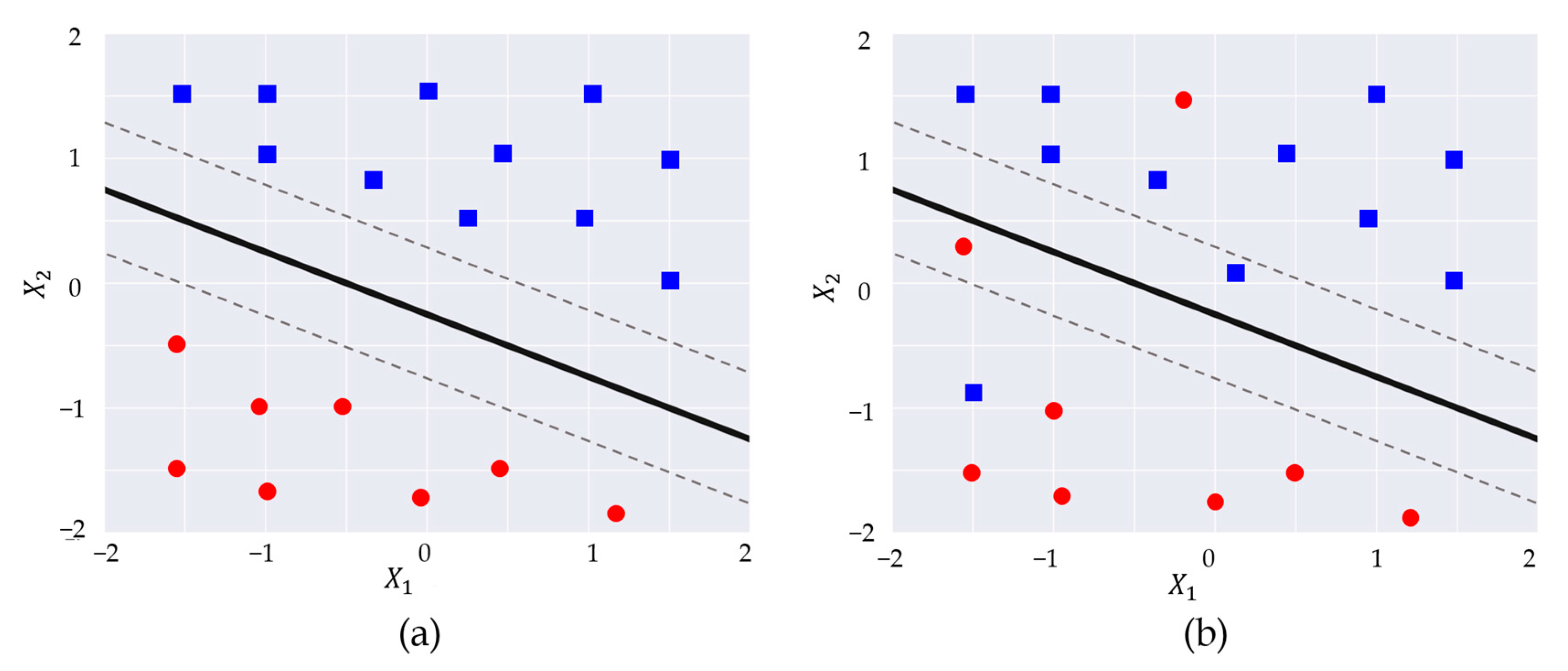
The support vector machine (SVM) algorithm is a method for classification and regression tasks [24]. For classification applications, the algorithm tries to find a hyperplane that separates the training observations according to their class labels with a maximum margin. Figure 2a shows a separating hyperplane corresponding to a “hard-margin” linear SVM (L-SVM) for a two-dimensional data space.

In this example of $n$ training observations split into two classes ($y_1,\dots ,y_n \in \left\{-1, 1\right\}$ where $-1$ represents one class and $1$ the other class), the training process consists of finding the hyperplane (defined by $\beta =\left\{{\beta }_0, {\beta }_1, {\beta }_2\right\}$ such as ${\beta }_0+{\beta }_1.X_1+{\beta }_2.X_2=0$), which is able to separate the training observations perfectly, as shown below.

$$\{\begin{array}{c}{\beta }_0+{\beta }_1.x_{i1}+{\beta }_2.x_{i2}>0 if y_i=1\\ {\beta }_0+{\beta }_1.x_{i1}+{\beta }_2.x_{i2}<0 if y_i=-1\end{array},$$

(3)

which is equivalent to

$$y_i.\left({\beta }_0+{\beta }_1.x_{i1}+{\beta }_2.x_{i2}\right)>0, \forall i=1, \dots , n$$

(4)

A test observation $x^{*}$ is classified based on the sign and the magnitude of $f\left(x^{*}\right)={\beta }_0+{\beta }_1.x_1^{*}+{\beta }_2.x_2^{*}$ as follows:

• If $f\left(x^{*}\right)$ is positive, the test observation is assigned the label $1$;
• If $f\left(x^{*}\right)$ is negative, $x^{*}$ is assigned to class $-1$;
• If $f\left(x^{*}\right)$ is far from zero, this means that $x^{*}$ is located far from the hyperplane. Thus, we can be confident about the class assignment for $x^{*}$;
• If $f\left(x^{*}\right)$ is close to zero, this means that $x^{*}$ is located near to the hyperplane. Thus, we are less certain about the class assignment for $x^{*}$;

Ideally, observations that belong to two classes are perfectly separable by a hyperplane (Figure 2a). In this case, the maximal margin hyperplane is the solution of the constrained optimization problem in Equation (5).

$$\{\begin{array}{c}\begin{array}{c}\mathit{m}\mathit{i}\mathit{n}\mathit{i}\mathit{m}\mathit{i}\mathit{z}\mathit{e}\\ {\mathit{\beta }}_{\mathbf{0}}\mathbf{,} {\mathit{\beta }}_{\mathbf{1}}\mathbf{,} {\mathit{\beta }}_{\mathbf{2}}\end{array} \frac{1}{2}\left({\beta }_1.X_1+{\beta }_2.X_2\right)\\ subject to\\ y_i.\left({\beta }_0+{\beta }_1.x_{i1}+{\beta }_2.x_{i2}\right)\ge 1 \forall i=1, \dots , n \end{array},$$

(5)

However, observations that belong to two classes are not always perfectly separable by a hyperplane (Figure 2b). In such cases, the separate hyperplane should be able to separate most of the training observations, while tolerating some misclassifications. This gives the constrained optimization problem in Equation (6).

$$\{\begin{array}{c}\begin{array}{c}\mathit{m}\mathit{i}\mathit{n}\mathit{i}\mathit{m}\mathit{i}\mathit{z}\mathit{e}\\ {\mathit{\beta }}_{\mathbf{0}}, {\mathit{\beta }}_{\mathbf{1}}\mathbf{,} {\mathit{\beta }}_{\mathbf{2}}\mathbf{,} {\mathit{\xi }}_{\mathbf{1} }\mathbf{,} \dots \mathbf{,}\mathbf{ }{\mathit{\xi }}_{\mathit{n}}\end{array} \frac{1}{2}\left({\beta }_1.X_1+{\beta }_2.X_2\right)+C.{{\displaystyle \sum }}_{i=1}^n{\xi }_i\\ subject to\\ y_i.\left({\beta }_0+{\beta }_1.x_{i1}+{\beta }_2.x_{i2}\right)\ge \left(1-{\xi }_i\right), \forall i=1, \dots , n \\ {\xi }_i\ge 0\end{array},$$

(6)

where

• C is a tuning parameter;
• ${\xi }_i$ are slack variables, allowing individual observations to be on the wrong side of the margin or the hyperplane;

The Radial Basis Function-Support Vector Machine (RBF-SVM) is a variant of the SVM algorithm. Contrary to the linear SVM based on a linear kernel, (i.e., a dot product between the feature vectors of two data points), the RBF-SVM uses a radial basis kernel (also known as a Gaussian kernel) to map the input data into a higher-dimensional feature space, in order to create more complex decision boundaries than can capture non-linear relationships between the features and the output. This gives the constrained optimization problem in Equation (7).

$$\{\begin{array}{c}\begin{array}{c}\mathit{m}\mathit{i}\mathit{n}\mathit{i}\mathit{m}\mathit{i}\mathit{z}\mathit{e}\\ {\mathit{\beta }}_{\mathbf{0}}\mathbf{,} {\mathit{\beta }}_{\mathbf{1}}\mathbf{,} {\mathit{\beta }}_{\mathbf{2}}\mathbf{,} {\mathit{\xi }}_{\mathbf{1} }\mathbf{,} \mathbf{\dots }\mathbf{,} {\mathit{\xi }}_{\mathit{n}}\end{array} \frac{1}{2}\left({\beta }_1^2+{\beta }_2^2\right)+C.{{\displaystyle \sum }}_{i=1}^n{\xi }_i\\ subject to\\ y_i.\left({\beta }_0+{{\displaystyle \sum }}_{j=1}^n{\beta }_j.K\left(x_i, x_j\right)\right)\ge \left(1-{\xi }_i\right), \forall i=1, \dots , n \\ {\xi }_i\ge 0\end{array},$$

(7)

where

• C is a tuning parameter;
• ${\xi }_i$ are slack variables, allowing individual observations to be on the wrong side of the margin or the hyperplane;
• $K\left(x_i, x_j\right)=exp(-\gamma .\Vert x_i-x_j{\Vert }^2$) measures the similarity between the feature vectors $x_i$ and $x_j$;
• $\gamma$ is the kernel parameter that controls the influence of the RBF kernel;

Drucker et al. extend the SVM algorithm in order to process regression tasks [25]. In this case, the algorithm does not intend to find a hyperplane to split the data into distinct classes. Instead, its aim is to identify a hyperplane that is as close as possible to the target values ($y_i)$. For example, the optimization problem in Equation (8) represents the specific case of a linear soft margin regression.

$$\{\begin{array}{c}\begin{array}{c}\mathit{m}\mathit{i}\mathit{n}\mathit{i}\mathit{m}\mathit{i}\mathit{z}\mathit{e}\\ {\mathit{\beta }}_{\mathbf{0}}, {\mathit{\beta }}_{\mathbf{1}}\mathbf{,} {\mathit{\beta }}_{\mathbf{2}}\mathbf{,} {\mathit{\xi }}_{\mathbf{1} }\mathbf{,} \mathbf{\dots }\mathbf{,} {\mathit{\xi }}_{\mathit{n}}\mathbf{,} {\mathit{\xi }}_{\mathbf{1} }^{\mathbf{*}}\mathbf{,} \mathbf{\dots }\mathbf{,} {\mathit{\xi }}_{\mathit{n} }^{\mathbf{*}}\end{array} \frac{1}{2}\left({\beta }_1.X_1+{\beta }_2.X_2\right)+C.{{\displaystyle \sum }}_{i=1}^n\left({\xi }_i+{\xi }_i^{*}\right)\\ subject to\\ y_i-\left({\beta }_0+{\beta }_1.x_{i1}+{\beta }_2.x_{i2}\right)\le \epsilon +{\xi }_i, \forall i=1, \dots , n\\ \left({\beta }_0+{\beta }_1.x_{i1}+{\beta }_2.x_{i2}\right)-y_i\le \epsilon +{\xi }_i^{*}, \forall i=1, \dots , n \\ {\xi }_i\ge 0, {\xi }_i^{*}\ge 0, \forall i=1, \dots , n \end{array}$$

(8)

where

• C is a tuning parameter;
• ${\xi }_i, {\xi }_i^{*}$ are slack variables.

It worth noting that Equation (8) can be generalized to the p dimensional space and process regression using multiple parameters, as shown in Equation (9).

$$\{\begin{array}{c}\begin{array}{c}\mathit{m}\mathit{i}\mathit{n}\mathit{i}\mathit{m}\mathit{i}\mathit{z}\mathit{e}\\ {\mathit{\beta }}_{\mathbf{0}}\mathbf{,} {\mathit{\beta }}_{\mathbf{1}}\mathbf{,}\mathbf{\dots }\mathbf{,} {\mathit{\beta }}_{\mathit{p}}\mathbf{,} {\mathit{\xi }}_{\mathbf{1} }\mathbf{,} \mathbf{\dots }\mathbf{,} {\mathit{\xi }}_{\mathit{n}}\mathbf{,} {\mathit{\xi }}_{\mathbf{1} }^{\mathbf{*}}\mathbf{,} \mathbf{\dots }\mathbf{,} {\mathit{\xi }}_{\mathit{n} }^{\mathbf{*}}\end{array} \frac{1}{2}\left({\beta }_1.X_1+\dots +{\beta }_p.X_p\right)+C.{{\displaystyle \sum }}_{i=1}^n\left({\xi }_i+{\xi }_i^{*}\right)\\ subject to\\ y_i-\left({\beta }_0+{\beta }_1.x_{i1}+\dots +{\beta }_p.x_{ip}\right)\le \epsilon +{\xi }_i, \forall i=1, \dots , n\\ \left({\beta }_0+{\beta }_1.x_{i1}+\dots +{\beta }_p.x_{ip}\right)-y_i\le \epsilon +{\xi }_i^{*}, \forall i=1, \dots , n \\ {\xi }_i\ge 0, {\xi }_i^{*}\ge 0, \forall i=1, \dots , n \end{array}$$

(9)

where

• C is a tuning parameter;
• ${\xi }_i, {\xi }_i^{*}$ are slack variables.

2.3. Decision Tree

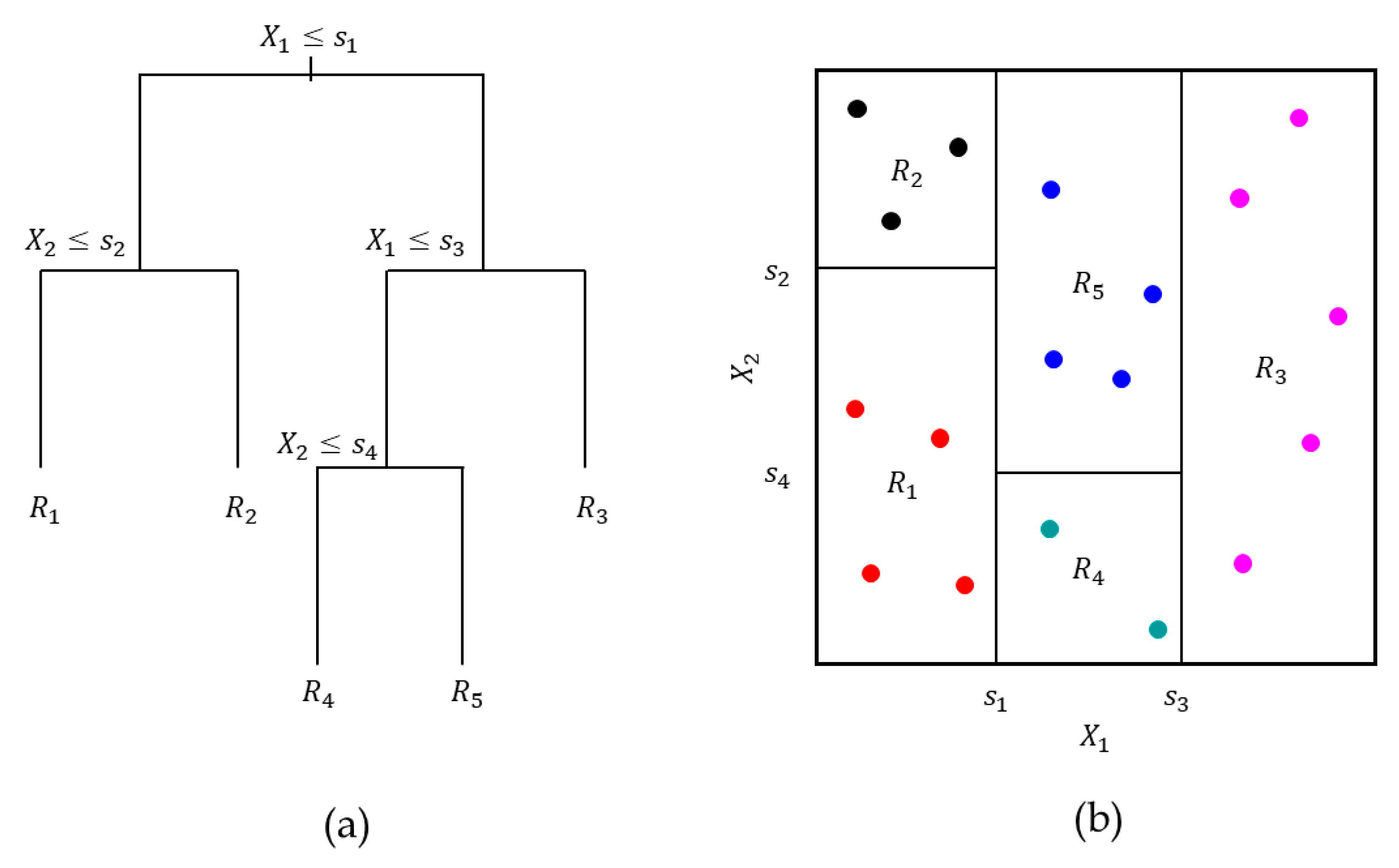
Decision trees can be applied to both regression and classification tasks [26,27]. They consist of a series of splitting rules (Figure 3a), starting at the top of the tree in order to make predictions by subdividing the feature space. As shown in Figure 3b, the aim of the decision tree is to divide the feature space $\left(X\right)$ into $N$ distinct and non-overlapping regions, where $R=\left\{R_{1 },\dots ,R_{N }\right\}$. During the training process, the splitting process is guided by metrics such as Gini index Equation (10) and entropy Equation (11), which measure the impurity or the disorder of a set of samples.

The test observations that fall into a region $\left(R_i\right)$ receive the same prediction, which corresponds to the mean of the target values of the training observations.

$$Gini index=1-{{\displaystyle \sum }}^{}{\left(p_i\right)}^2$$

(10)

$$Entropy=-\left({{\displaystyle \sum }}^{}{p}_i.lo{g}_2\left(p_i\right)\right)$$

(11)

where

• $p_i$ is the proportion of samples belonging to class i.

3. Dataset Description

The data for this study were obtained from an extensive test campaign, carried out within the European VERT project [28]. These tests involved using a fifth-wheel device to measure the coefficient of friction on different road surfaces at different slip ratios, vehicle speeds, tire tread depths and water depths (

Table 1. Experimental conditions investigated.

Parameters	Unity	Values
Speed	km/h	20–40–50–60–80–90
MPD	mm	0.48–0.72
Water depth	mm	1–3–8
Tire tread depth	mm	2–4–8

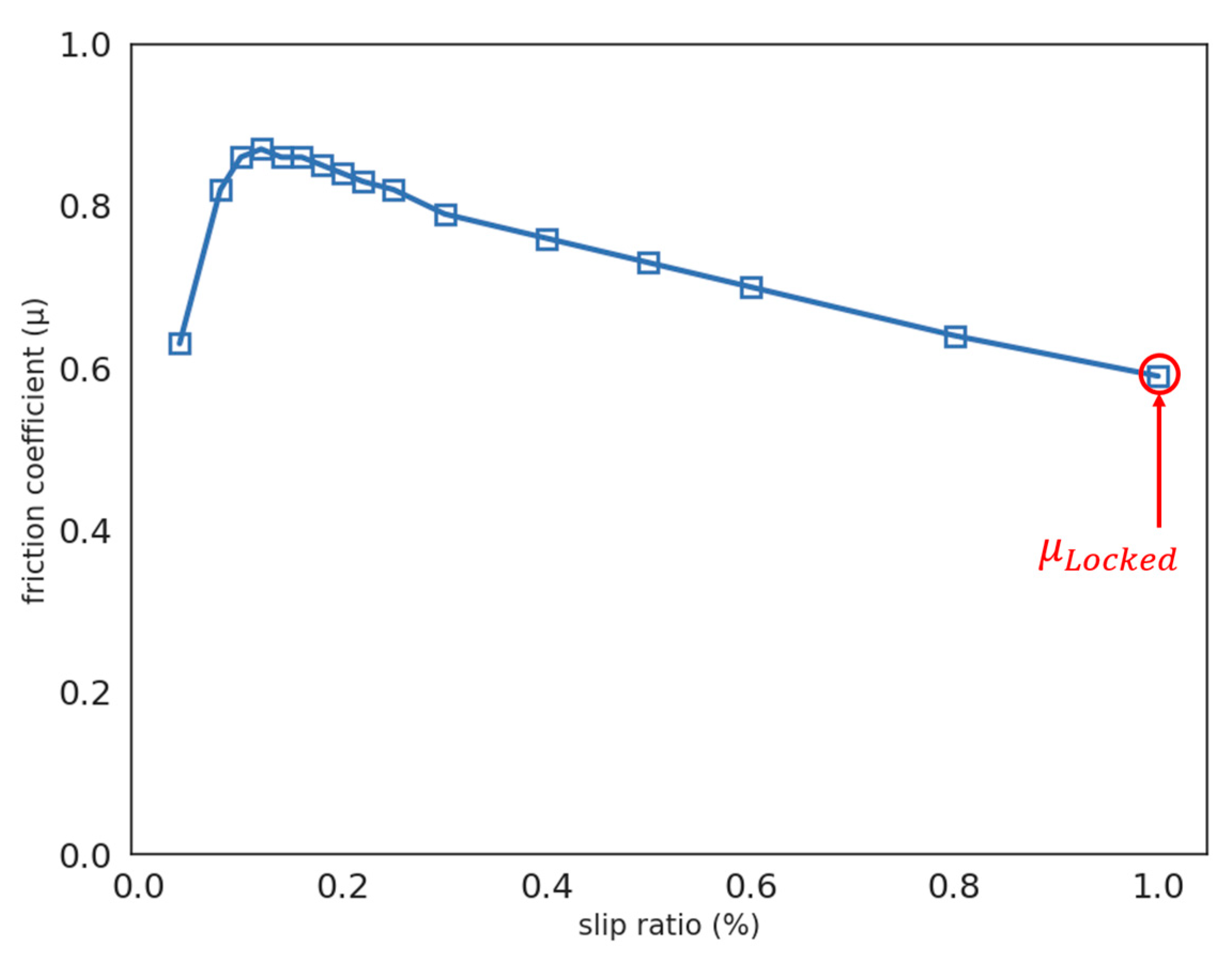
). The test surfaces, named $S_1$ and $S_2$ respectively, are characterized by their macrotexture, expressed in terms of Mean Profile Depth (MPD). $S_1$ is a surface dressing with an MPD of 0.48 mm; $S_2$ is an asphalt concrete with an MPD of 0.72 mm. Pirelli summer tires 195/65 R15, inflated at 0.22 MPa, were used. Ambient temperature was not recorded but all tests were performed within a few days to maintain the same weather conditions. For each experiment, values of the coefficient of friction at 100% of the slip ratio (µ locked, Figure 4) were extracted and formed the target prediction data. The data set containing 102 samples was split into a training set of 71 samples and a validation set of 31 samples.

It should be noted that the analysis of peak coefficients of friction could be more intuitive, considering the fact that vehicles nowadays dispose of ABS systems. However, as the locked-wheel coefficient of friction better highlights the effect of influencing factors, it was thought that locked µ values would be more relevant to compare ML algorithms.

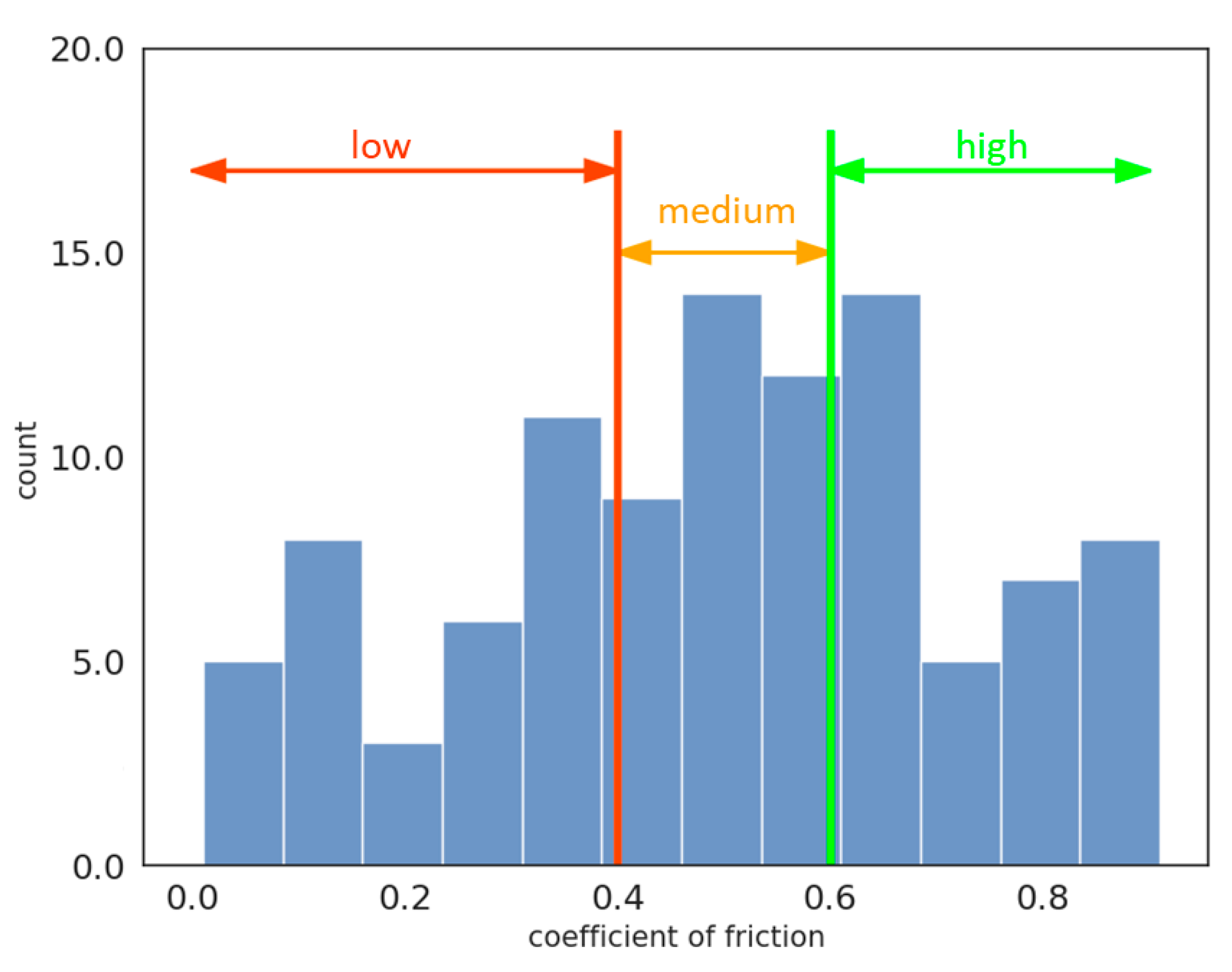
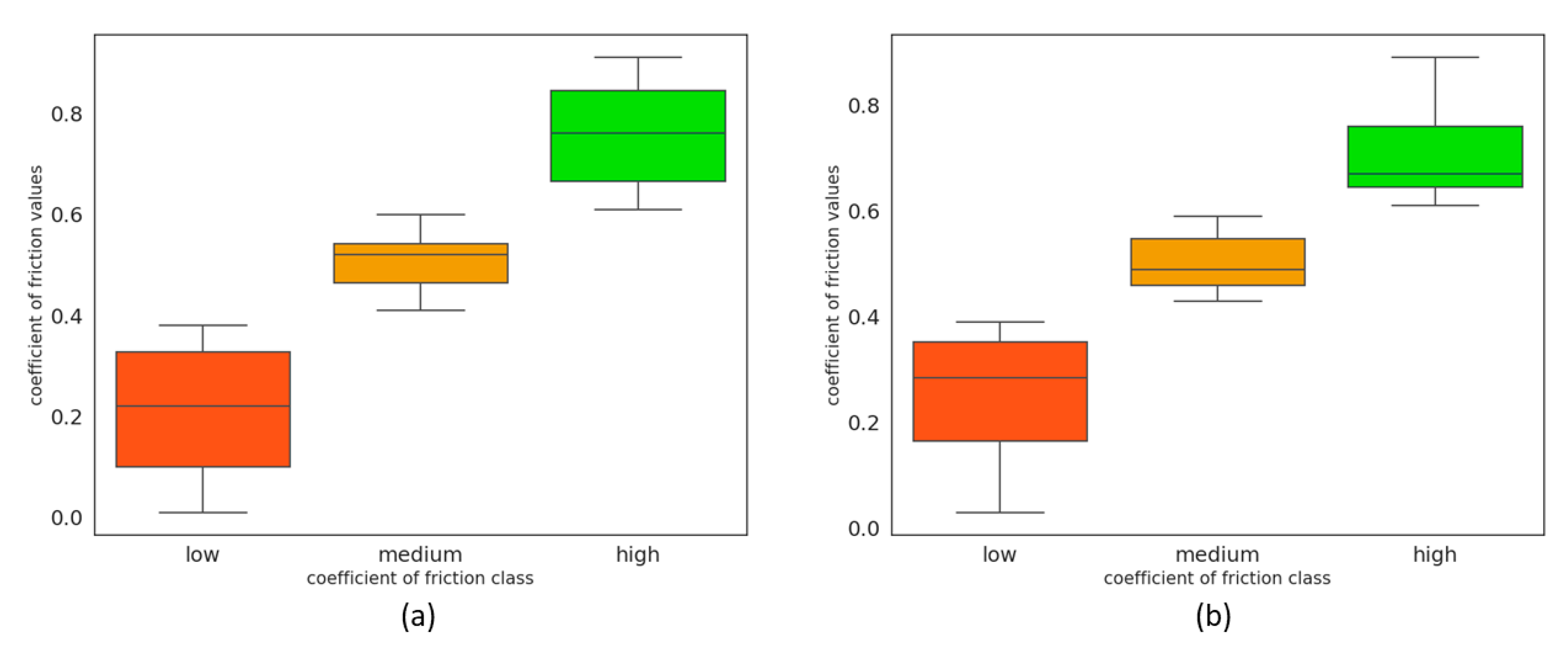
The investigation of skid resistance prediction from a classification perspective involves splitting the target data (friction coefficient values) into three classes (Figure 5), with threshold values chosen based on the literature [29,30,31]:

• The low-skid resistance class corresponding to friction coefficient values below 0.4;
• The medium-skid resistance class corresponding to friction coefficient values between 0.4 and 0.6;
• The high-skid resistance class corresponding to friction coefficient values higher than 0.6.

The distributions of the three classes (low–medium–high) between the training (71 samples) and the testing (31 samples) data set are presented in Figure 6 and summarized in

Table 2. Distribution of skid resistance classes between the training and testing data set.

Class	Low	Medium	High
All data	34	34	34
Training	24	24	23
Testing	10	10	11

.

Certain ML algorithms (SVM, neural networks, etc.) can be sensitive to the scale of data values, which may affect their performance. To address this issue, the dataset was normalized using min–max scaler function Equation (12). This pre-processing stage ensures that all features are appropriately scaled to lie within the range of 0 and 1.

$$X_{scaled}=\frac{X-X_{min}}{X_{max}-X_{min}},$$

(12)

where

• $X$ and $X_{scaled}$ represent the original and transformed feature values, respectively.
• $X_{min}, X_{max}$ represent the minimum and maximum feature values, respectively.

4. Results Analysis

The following calculations were made using the ML toolbox scikit-learn implementation [32]. The paragraphs below present the results of the regression study, divided into linear (MLR, linear SVM) and non-linear (D.T, RBF-SVM) methods.

4.1. Regression Analysis

4.1.1. Linear Methods

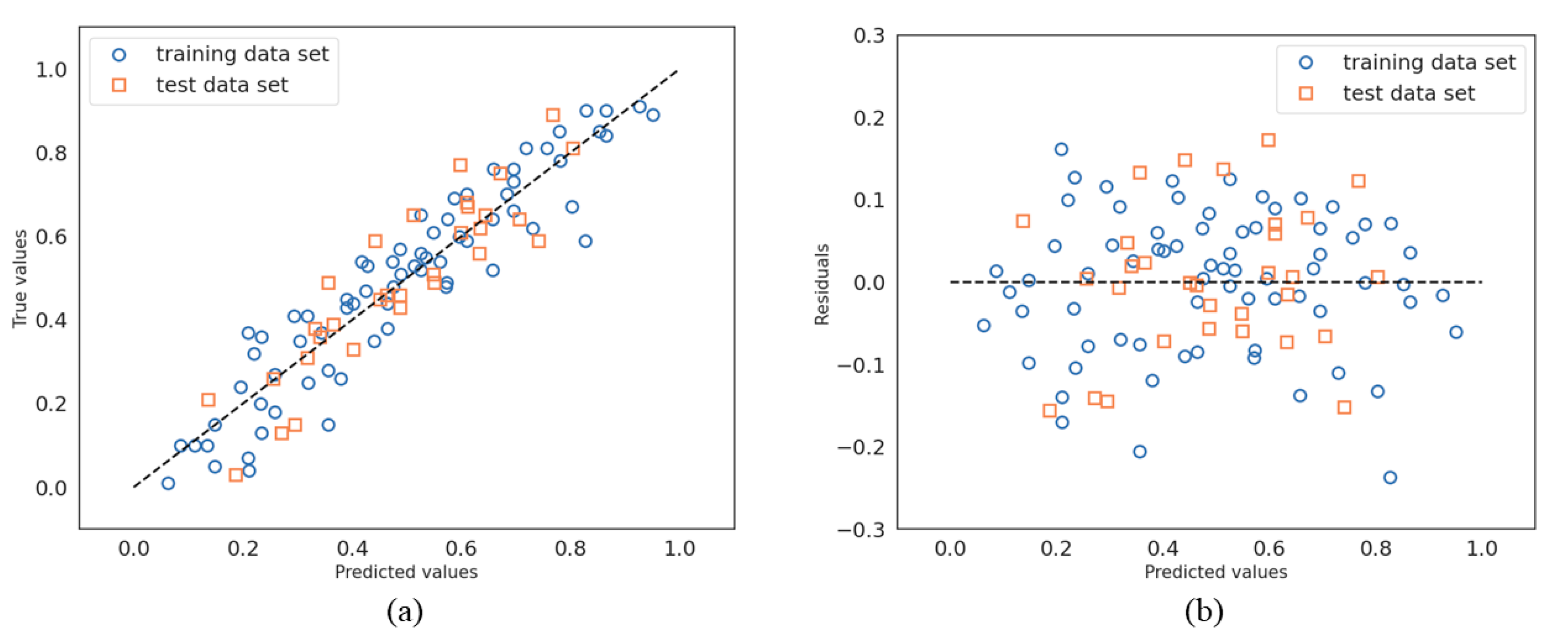
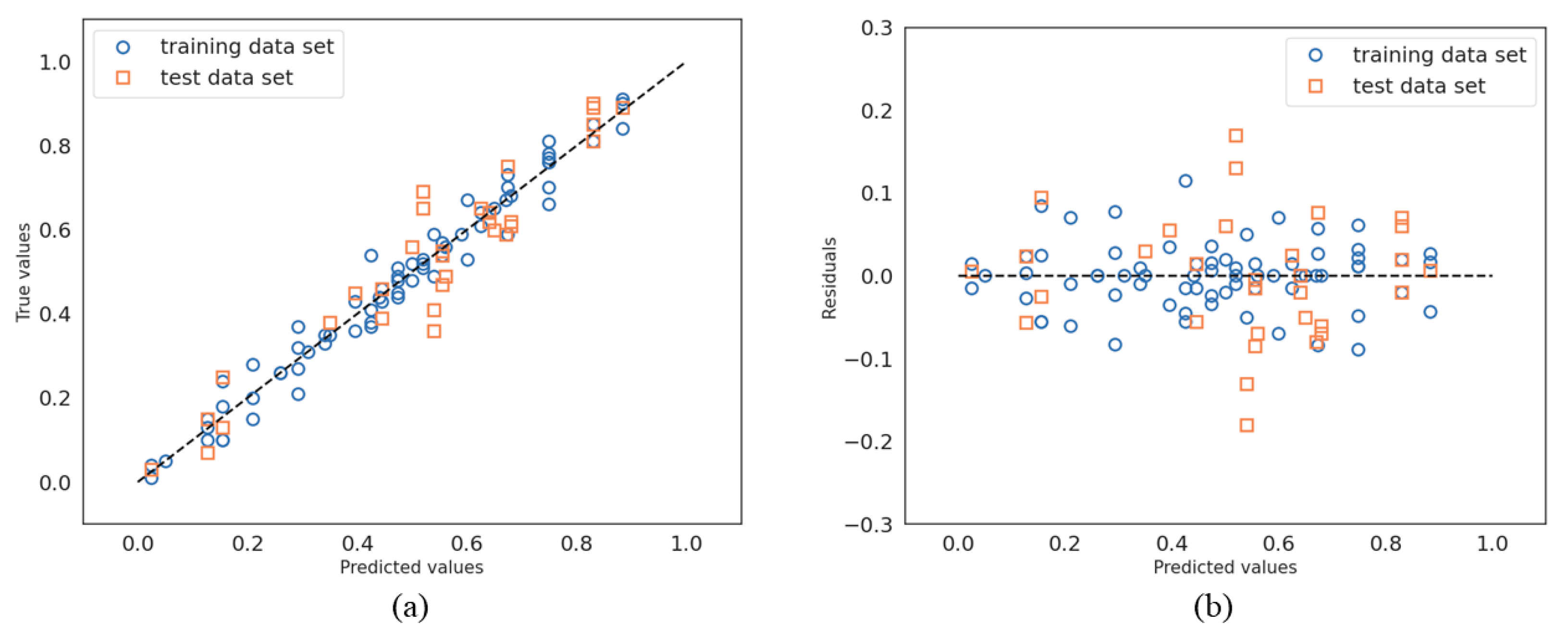
Figure 7 shows the regression (Figure 7a) and the residual (Figure 7b) results for both the training and testing data sets for the multiple linear regression method. In Figure 7a (a plot of true values versus predicted values), we observe that the training and testing values are uniformly distributed along the diagonal line (in dot points). This is synonymous with good regression quality for both training and testing data sets. This impression is confirmed by the residual plot (Figure 7b) in which the majority of the residual values are distributed within the range of −0.2 to 0.2.

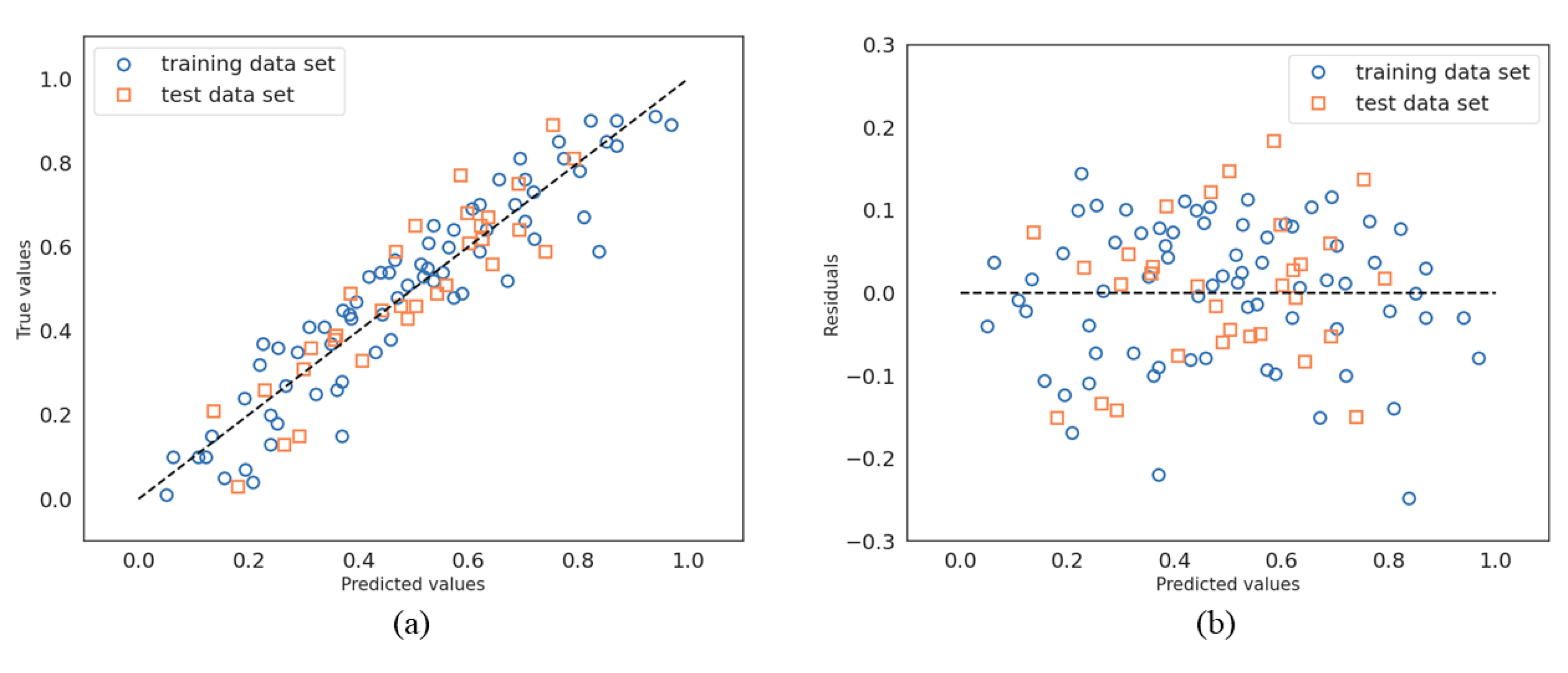
As shown in Figure 8a,b, the regression and residual plots for linear SVMs are quite similar to those from the multiple linear regression method. This observation is confirmed by $R^2$ (coefficient of determination) and $RMSE$ (root mean square error) values (summarized on

Table 3. $R^2$ and $RMSE$ for linear methods.

Algorithms	R2		RMSE
	Train	Test	Train	Test
MLR	0.877	0.818	0.282	0.315
Linear SVM	0.87	0.82	0.29	0.31

), which are very close for both the training and testing data set. This is due to the fact both algorithms assume a linear relationship between the target variable and the features. However, the advantage of the linear SVM over OLS linear regression lies in its ability to minimize overfitting concerns, especially when dealing with noisy data [33].

4.1.2. Non-Linear Methods

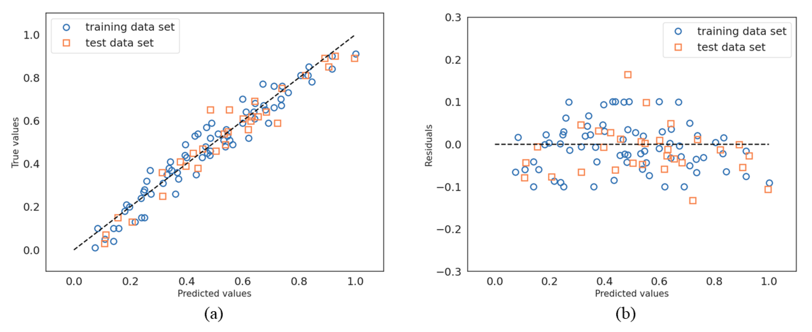
Figure 9 and Figure 10 present the results of regression and residuals for the two non-linear methods investigated. As shown in

Table 4. $R^2$ and $RMSE$ for non-linear methods.

Algorithms	R2		RMSE
	Training	Testing	Training	Testing
RBF SVM	0.94	0.93	0.24	0.24
DT	0.96	0.91	0.2	0.27

, both algorithms provide better results than the linear ones, which is an indication that the relationship between the features and the target is non-linear.

This assumption is confirmed by the residual plots, where most of the points are distributed within the range of −1.2 to 1.2. Three observations can be made:

• Even the $R^2$ and $RMSE$ values are distributed close together for the RBF-SVM and the decision tree and it is obvious that the RBF-SVM provides slightly better regression results than the DT.
• A closer look at the values of the training and testing values of $R^2$ for the RBF-SVM (0.94 and 0.93) and the D.T (0.96 and 0.91) indicates the better generalizing capability of the RBF-SVM compared to the decision tree from small training data sets.
• In Figure 10a, we note that the decision tree algorithm has a distinguish “signature” compared to the other algorithms. The algorithm provides the same predicted value for different instances. This gives the plot (true versus predicted values) a vertically stratified aspect.

4.2. Classification Analysis

In the following paragraphs, the results of three classification algorithms ((1) linear SVM, (2) RBF-SVM and (3) decision tree) are described in terms of visual representation, confusion matrix, and precision–recall–f score metrics.

4.2.1. Visual Representation Analysis

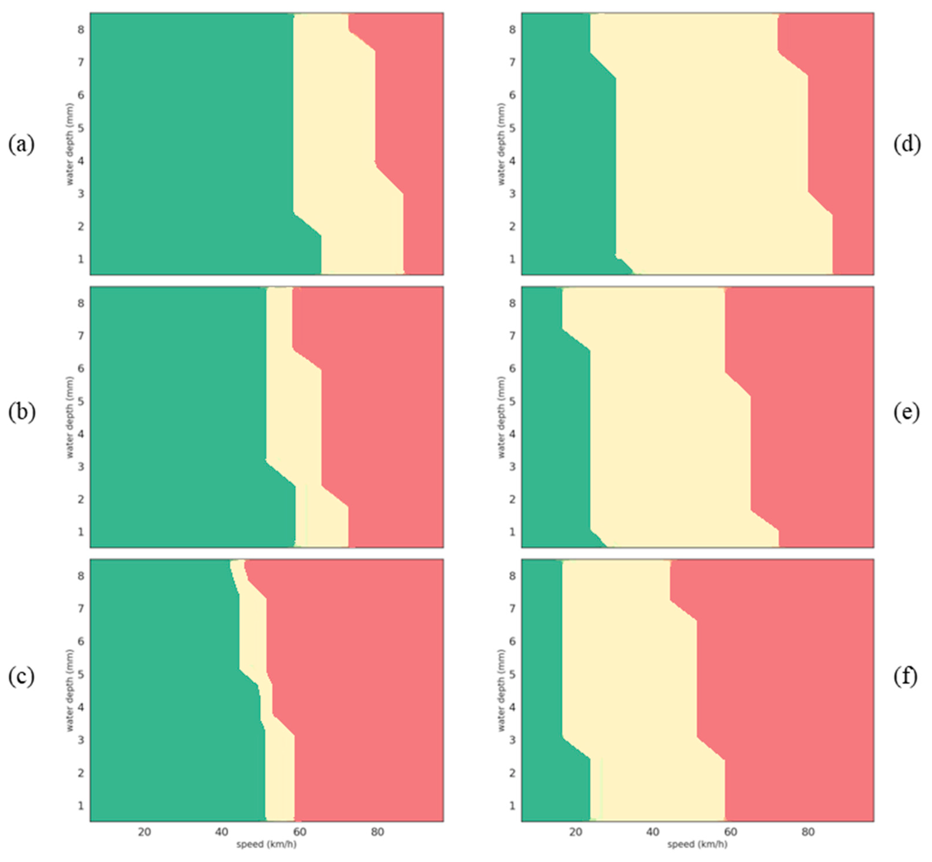
In this section, classification results are presented in the form of a map representing variations in the coefficient of friction due to changes in the water depths and vehicle speeds, for fixed values of macrotexture and tire tread depth. As shown in Figure 11, each map is segmented into three distinct color-coded areas (green, yellow and red), corresponding to the high-, medium- and low-skid resistance classes, respectively.

Figure 12 presents the results of linear SVM classification algorithm in the form of six graphs:

• Figure 12a–c present classification results (in the form of water depth change according to vehicle speed change) for surface $S_1$ (MPD of 0.48 mm) at different tire tread depths (8, 4 and 2 mm, respectively).
• Figure 12d–f present classification results (in the form of water depth change according to vehicle speed change) for surface $S_2$ (MPD of 0.72 mm) at different tire tread depths (8, 4 and 2 mm, respectively).

The main observations are as follows:

• When the vehicle speed increases, for any water depth, the skid resistance class changes from high (green) to medium (yellow) and then low (red). This observation is consistent as it has been well established that the tire/wet road friction decreases when the vehicle speed increases [34].
• The effect of water depth on the distribution of classes is less obvious to interpret but still makes sense. At a given speed, increasing the water depth can have no effect at low speed (for example, at 40 km/h in Figure 12a) or degrades the skid resistance class (for example, in Figure 12a, for a vehicle speed of 80 km/h, the skid resistance class changes from medium to low when the water depth increases).

As explained in [35], at low speeds, a tire tread element crossing the tire–wet road contact area has enough time to descend through the water film and make contact with the road surface; as a result, the coefficient of friction is generally high. On the other hand, as water lubricates the tire/road interface, increasing the water depth has an adverse effect on skid resistance mainly when the vehicle speed is high [36,37]; as a result, the skid resistance class can degrade.

• The effect of the tire tread depth can be seen from the comparison of Figure 12a–c on one side or Figure 12d–f on the other side; new tires help to reduce the extension of the low-skid resistance area (in other words, low-skid resistance can only be reached at high speeds), even if the benefit is lessened when the water depth increases.

Conversely, worn tires not only speed up the deterioration of skid resistance but also make the transition from safe (green area) to unsafe (red area) more abrupt (Figure 12c).

• The effect of the surface macrotexture depends on the test speed. The distribution of low-skid resistance classes is the same (comparison of Figure 12a versus Figure 12d, Figure 12b versus Figure 12e, and Figure 12c versus Figure 12f). The main difference between the two surfaces is the relative fraction of high- and medium-skid resistance classes.

When the test speed increases, the green area is larger than the yellow one for surface $S_1$ and the reverse is true for surface $S_2$. It means that moving on surface $S_1$ is safe at low speed (up to 40 km/h). However, as shown in Figure 12c, due to the narrow width of the medium class (yellow), the skid resistance can significantly decrease when the vehicle speed increases further, mainly when the tires are worn. On surface $S_2$, the skid resistance is most of the time part of the medium class and the transition from medium to low is smoother.

The behavior of the two test surfaces can be explained by their macrotexture, expressed as a Mean Profile Depth, and their microtexture, which was not a variable of the test program. Using a low-speed coefficient of friction, which is a common indirect indicator of road surface microtexture, we obtained 0.69 and 0.48 for surfaces $S_1$ and $S_2$, respectively [38], which means that $S_1$ has a higher microtexture than $S_2$. Surface $S_1$ is, therefore, a high-microtexture (0.69)/low-macrotexture (0.48) surface, whereas $S_2$ is a low-microtexture (0.48)/high-macrotexture surface (0.72).

As mentioned in the work of Hall et al. [39], a high-microtexture surface ($S_1$) has a high-skid resistance at low speeds (until 40 km/h); however, if its macrotexture is low, skid resistance can significantly decrease when the vehicle speed increases further. The lower skid resistance of surface $S_2$ is due to its low microtexture; however, it remains stable with respect to the vehicle speed thanks to its high macrotexture.

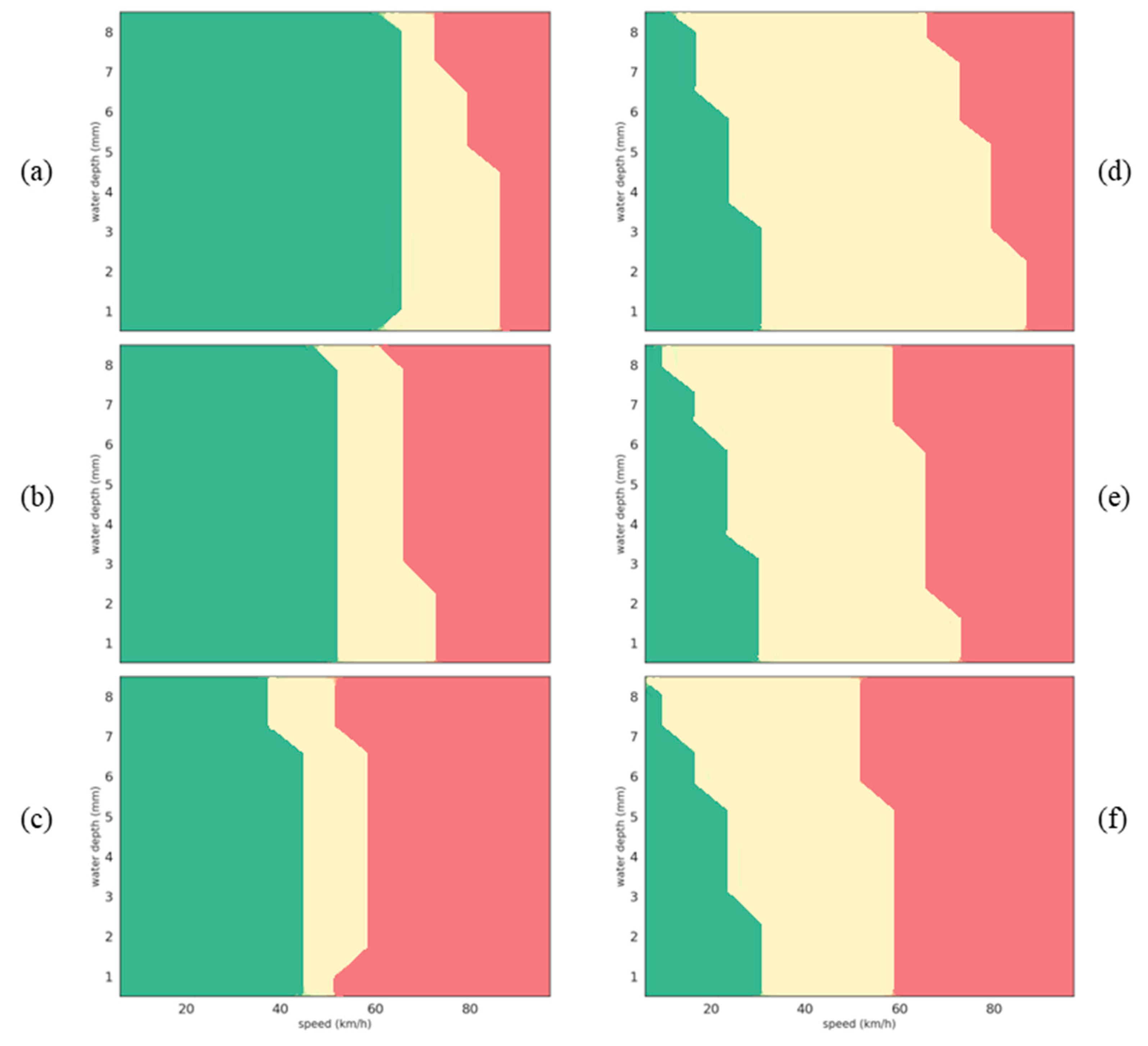
Most of the observations made previously concerning the distribution of skid resistance classes can be applied to the RBF-SVM classification algorithm (Figure 13). The minor differences are as follows:

• The transition from high- to low-skid resistance class is less abrupt for worn tires (Figure 12c versus Figure 13c).
• On surface $S_2$, the effect of water depth is more visible on the extension of the high-skid resistance class (reduction in the green area when the water depth increases) (Figure 13d–f).

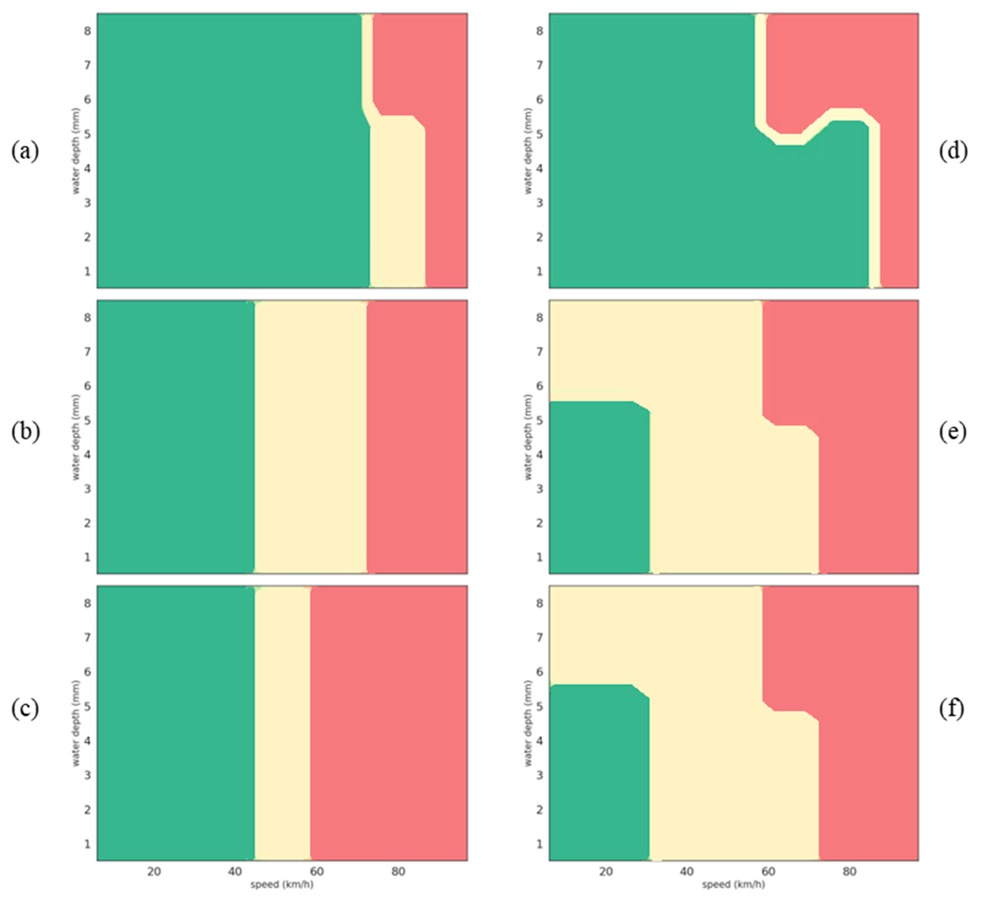
Concerning the decision tree classification algorithm, the results seem less relevant than the two SVM algorithms:

• In fact, when the vehicle speed increases with new tires on surface $S_2$ (Figure 14d), the change in skid resistance classes is unexpected at water depths of around 5–6 mm: based on the lubrication action of water at the tire–road interface, the coefficient of friction cannot increase with the vehicle speed.
• Another point is that Figure 14e,f are identical, which means that the algorithm provides the same prediction for two different driving conditions: (1) tire tread depth = 4 mm, MPD = 0.72 mm and (2) tire tread depth = 2 mm, MPD = 0.72 mm. A similar observation was made in the regression study results (Section 4.1.2, Figure 10a).

This last point can be explained by the limitations inherent to the algorithm structure, i.e., discretization of the feature space. Indeed, the decision trees partition the feature space into distinct regions using thresholds. The predicted value within each region is determined by the majority or average of the training samples falling into that region.

This implies that instances that are similar or present very close features will receive the same predicted value or class. This is particularly relevant when decision trees are trained on limited data or if the training data lack diversity in certain regions of the feature space. In this situation, the tree structure may not have enough information to accurately differentiate between instances with similar feature values, leading to identical predictions for different instances.

4.2.2. Confusion Matrix and Metrics (Precision, Recall, F1 Score) Analysis

Table 5. Confusion matrix for linear SVM.

		Predicted Label
True label	Class	Low	Medium	High
	Low	8	2	0
	Medium	1	7	2
	High	0	2	9

,

Table 6. Confusion matrix for RBF-SVM.

		Predicted Label
True label	Class	Low	Medium	High
	Low	8	2	0
	Medium	1	9	0
	High	0	2	9

and

Table 7. Confusion matrix for decision tree.

		Predicted Label
True label	class	low	medium	high
	low	8	2	0
	medium	1	9	0
	high	0	3	8

present the confusion matrices for linear SVM, RBF-SVM and decision tree algorithms. The results show misclassification errors of 7, 5 and 6 samples for linear SVM, RBF-SVM and decision tree algorithms, respectively. This leads to a mean accuracy of 0.77, 0.84 and 0.81 for linear SVM, RBF-SVM and decision tree algorithms, respectively.

However, the mean accuracy, which gives a global view of the algorithm performances, remains insufficient to properly evaluate the algorithm predictions. Indeed, a misclassification due to an underestimation of the skid resistance level (for example, the algorithm predicts the low class red, while the actual class is medium yellow) is obviously less dangerous than an overestimation. Precision Equation (13), recall Equation (14), and f1-score Equation (15) are the most suitable metrics for the performance evaluation of a classification algorithm.

• Precision measures the proportion of correct predictions among all the predictions. Precision can be seen as an indicator of quality. Indeed, a high value of precision implies a low rate of false positive predictions. This means that the predictions provided by the model are more likely to be correct.
• Recall refers to the ability of the model to find all the expected objects within the dataset. Recall can be seen as an indicator of quantity. Indeed, a high value of recall implies a low rate of false negative predictions. This means that the model is more likely to find all the pertinent items.
• The F1-score or f-measure is defined as the harmonic mean of precision and recall.

$$precision=\frac{TP}{TP + FP},$$

(13)

$$recall = \frac{TP}{TP + FN},$$

(14)

$$f1 score = 2 \times \frac{precision \times recall}{precision + recall},$$

(15)

where

• $TP$, true positives;
• $FN$, false negatives;
• $FP$, false positives.

The precision (

Table 8. Precision values for the algorithms studied.

Class	L-SVM	RBF-SVM	D.T
Low	0.89	0.89	0.89
Medium	0.64	0.69	0.64
High	0.82	1.0	1.0

), recall (

Table 9. Recall values for the algorithms studied.

Class	L-SVM	RBF-SVM	D.T
Low	0.80	0.80	0.80
Medium	0.70	0.90	0.90
High	0.82	0.82	0.73

) and f1-score (

Table 10. f1-score values for the algorithms studied.

Class	L-SVM	RBF-SVM	D.T
Low	0.84	0.84	0.84
Medium	0.67	0.78	0.75
High	0.82	0.90	0.84

) values according to the different classes show that the RBF-SVM algorithm, while performing as well as the DT and L-SVM for low class prediction, outperforms both these algorithms when it comes to predicting medium- and high-skid resistance classes.

5. Discussion

Predicting skid resistance remains a challenging task due to the variety of factors involved. This study conducted under controlled conditions close to the real conditions focused on the evaluation of tire tread depth, water depth, vehicle speed and pavement macrotexture as influencing parameters. Despite the relatively small size of the dataset, both prediction and classification studies provide promising results. It was observed that the RBF-SVM algorithm, due to its ability to map the features into a higher dimension space to deal with the non-linear phenomenon, outperforms OLS linear regression, L-SVM and decision tree algorithms for the regression task and L-SVM and decision tree algorithms for the classification task.

In comparison to the amount of studies referring to Artificial Intelligence methods for the detection of surface distresses (cracking, patching, potholes, surface deformation, and others) [40,41,42], there is a noticeable lack of research works that address skid resistance prediction. Furthermore, the existing studies differ from the present work in terms of investigated inputs (features) and data set size. Consequently, it becomes quite challenging to discuss the results of this study in the context of the available literature. To illustrate this point, we can refer to the following studies:

• Marcelino et al. conducted a study that can be considered as a precursor in this research field [43]. They utilized the Long-Term Pavement Performance (LTPP) database to assess the effectiveness of two Machine Learning models (linear regression and regularized regression with lasso) in predicting the skid resistance through regression analysis. Making a direct comparison between their work and ours is a difficult task due to the significant disparities in the input variables. Indeed, in our study, we focused on the vehicle speed, pavement macro-texture, tire tread depth and water depth, whereas Marcelino et al. utilized variables such as total monthly precipitation, average monthly temperature, international roughness index, accumulated traffic and other variables. However, it should be noted that Marcelino et al. achieved a slightly better result using the regularized regression ($R^2=0.583$) than the linear regression ($R^2=0.574$).
• Zhan et al. undertook a comparative study between conventional Machine Learning methods, such as support vector machines (SVM), k-nearest neighbors (KNN), and Gaussian Naïve Bayes (GNB), random forest (RF), and a modified version of the ResNets [44] architecture called Friction-ResNets, to predict skid resistance [45]. Although the prediction target was friction coefficient values (obtained with a grip tester), the input data consisted of pavement texture measurements. The work of Zhan et al. has shown that Friction-Resnets achieve a higher level of accuracy (91%) compared to SVM (81%), RF (78%), KNN (68%) and GNB (21%). Nevertheless, this outcome should be put into perspective with the size of the dataset used in this study (33,600 pairs of data divided into training (70%), testing (15%), and validation (15%) sets).
• Similarly to the approach taken by Zhan et al., Hu et al. performed a study to evaluate the effectiveness of some various Machine Learning models (LightGBM-light gradient boosting machine, XGBoost-extreme gradient boosting, SVM–support vector machine; RF–random forest) in predicting pavement skid resistance based on 3D surface macrotexture as input data [19]. Through regression analysis, their outcomes indicate that the Bayesian-LightGBM model achieves a higher coefficient of determination (0.93) compared to LightGBM (0.90), XGBoost (0.79), SVM (0.79) and RF (0.75).

The works mentioned above underscore the fact that, in the Machine Learning field, it is difficult to clearly identify a model that consistently excels across all scenarios. Indeed, each ML model is characterized by its strengths and limitations. Consequently, the performance of each model can vary depending on the dataset (quantity/quality), the features (input data), the target (output data), the task (regression/classification), the type of learning (supervised/unsupervised), and other factors.

In summary, the outcomes of a study cannot be straightforwardly applied to other works that utilize different input data and provide different outputs (regression versus classification), as the used data set may differ in quantity, quality, data aggregation methods, and contextual factors.

Recently, Roychowdhury et al. explored the concept of utilizing classification algorithms to predict skid resistance. Using front-camera images, the authors develop a two-stage classifier [46]:

• The first stage classifier consists of an artificial neural network (ANN) for the road surface condition (RSC) classification, which is able to identify four classes of road pavement condition: (1) dry, (2) wet/water, (3) slush, (4) snow/ice.
• The second stage consists of a road surface estimate (RFE) classification model to determine three levels of skid resistance: (1) a low RFE value corresponds to patchy snow and dry surfaces, which can result in slippery road conditions, (2) a medium RFE value signifies a partially patchy road and a high RFE value indicates a well-ploughed road.

Although skid resistance has been estimated indirectly (by assessing the level of contaminants on the road surface), this work demonstrates that a classification approach is as relevant as a regression analysis when it comes to estimating pavement skid resistance. It is worth mentioning the complementary aspect of the approach proposed by Roychowdhury et al. and our study. While Roychowdhury et al.’s work did not evaluate significant factors affecting skid resistance like tire wear or vehicle speed, our study only focused on water as a contaminant. An intelligent fusion of the outputs of both models can lead to a more robust and reliable model.

A critical aspect of this study lies in the relatively small size of the dataset used, consisting of only 102 samples. This limited dataset size introduces the possibility of dataset bias, wherein the training data may not adequately represent all real-world scenarios, resulting in poor generalization of the model. To address this concern effectively, one potential solution is to introduce synthetic data that accurately reflect real-world situations. By combining this synthetic data with the real dataset during training, we can enhance the model’s ability to adapt to diverse situations and improve its overall performance.

The importance of the ratio of synthetic data in the training mix was demonstrated by Jaipuria et al., who found that incorporating 40–60% synthetic data significantly enhances the model’s precision [47]. Adopting a similar approach in our study, using the integrated tire–vehicle–pavement modeling approach developed by Liu et al. [48] could lead to further improvements in the model’s performance.

It is worth noting that the current work has the following two limitations:

• The first limitation is related to the non-inclusion of crucial parameters such as the type of contaminant (water, snow, ice), road properties (slope, tilt, curvature), vehicle type (truck, motorcycle, etc.) and other factors. Incorporating these features can lead to a more complete, reliable and accurate model.
• The second limitation concerns the feasibility of incorporating these models into commercial vehicles. Indeed, specific sensors such as water depth measurement sensors and tire depth sensors are not available in commercial cars. However, the research on these topics shows promising progress. For example, the tire manufacturer Continental is working on the development of a sensor that can measure tire tread depth [49]. Additionally, experimental studies are currently being conducted to evaluate the feasibility of estimating water depths on road surfaces using accelerometric signals [50]. These works open new possibilities for the future of skid resistance estimation.

6. Conclusions

Despite the growing interest in applying Artificial Intelligence-based methods to pavement studies, limited research has been dedicated to skid resistance. Another missing gap is that users (engineers, authorities, etc.) are faced with a wide range of methods and it is challenging to choose the appropriate ones for their application. To address these gaps, this paper aimed to provide a comprehensive comparison of some popular Machine Learning models used to predict wet tire/road friction through regression and classification studies.

In the regression study, the two non-linear methods investigated (RBF-SVM and DT) outperformed the linear methods (linear SVM and MLR). This indicates that the relationship between the skid resistance and the features (vehicle speed, tire tread depth, water depth and pavement macro-texture) is non-linear. Furthermore, the RBF-SVM exhibited superior generalization capability compared to the DT.

The investigation of skid resistance prediction from a classification perspective involved splitting the target data (friction coefficient values) into three classes (low-, medium- and high-skid resistance class). The results demonstrated that the RBF-SVM algorithm performed as well as the DT and linear SVM for low class prediction, but outperformed both algorithms for predicting medium- and high-skid resistance classes. Additionally, this study illustrated a weakness of decision trees, when they were trained on limited data or if the training data lacked diversity in certain regions of the feature space. In such cases, the tree structure may not have enough information to accurately differentiate instances with similar feature values, leading to identical predictions for different instances.

In summary, from a relatively small dataset, this work demonstrated that the RBF-SVM model, with its ability to map the feature space in a high dimension to handle non-linear relationships between variables, is the most adapted tool for both regression tasks or classification tasks. This comparison must continue to include factors like the type of contaminants, traffic or weather conditions in order to build a more robust and reliable model.

This study has clearly established the necessity of incorporating domain expertise into Machine Learning-based approaches. While a Machine Learning model may provide a satisfactory overall performance, some of its individual outcomes can be inconsistent with the underlying physics of the studied phenomenon. This work has illustrated such inconsistencies in the classification task when the decision tree algorithm was used. By taking into account domain expertise, it becomes possible to assess the relevance of a model’s predictions with respect to reality.