Enhancing Quality Control of Chip Seal Construction through Machine Learning-Based Analysis of Surface Macrotexture Metrics

Abstract

Efforts to enhance quality control (QC) practices in chip seal construction have predominantly relied on single surface friction metrics such as mean profile depth (MPD) or friction number. These metrics assess chip seal quality by targeting issues such as aggregate loss or excessive bleeding, which may yield low friction numbers or texture depths. However, aggregate loss, particularly due to snowplow operations, does not always result in slippery conditions and may lead to uneven surfaces. The correlation between higher MPD or friction number and superior chip seal quality is not straightforward. This research introduces an innovative machine learning-based approach to enhance chip seal QC. Using a hybrid DBSCAN-Isolation Forest model, anomaly detection was conducted on a dataset comprising 183,794 20 m MPD measurements from actual chip seal projects across six districts in Indiana. This resulted in typical 20 m segment MPD ranges of [0.9 mm, 1.9 mm], [0.6 mm, 2.1 mm], [0.3 mm, 1.3 mm], [1.0 mm, 1.7 mm], [0.6 mm, 1.9 mm], and [1.0 mm, 2.3 mm] for the respective six districts in Indiana. A two-step QC procedure tailored for chip seal evaluation was proposed. The first step calculated outlier percentages across 1-mile segments, with an established limit of 25% outlier segments per wheel track. The second step assessed unqualified rates across projects, setting a threshold of 50% for unqualified 1-mile wheel track segments. Through validation analysis of four chip seal projects, both field inspection and friction measurements closely aligned with the proposed methodology’s results. The methodology presented establishes a foundational QC standard for chip seal projects, enhancing both acceptance efficiency and safety by using a quantitative method and minimizing the extended presence of practitioners on roadways.

1. Introduction

Chip sealing is a common surface treatment used to preserve and protect existing hot mix asphalt (HMA) pavements [1,2]. Its process involves applying a layer of asphalt emulsion on the pavement, followed by a layer of aggregate chips, which are compacted to create a durable and skid-resistant surface. A fog seal may be applied following chip seal application to help lock aggregate chips and reduce dust [3,4]. Chip seals offer substantial savings in both initial construction and long-term maintenance costs [5]. The application process of chip seals is relatively simple and requires less specialized equipment and labor compared to more extensive treatments like microsurfacing and thin or ultra-thin asphalt overlay. By sealing cracks, improving skid resistance, and protecting the pavement from water damage, chip sealing acts as a preventative maintenance measure that extends the life of existing pavements and reduces or delays the need for costly repairs or reconstruction in the future. Furthermore, chip sealing can be completed relatively quickly, minimizing road closures and disruptions to traffic that further enhance its cost-effectiveness.

The right choice of aggregate and precise application rates for both aggregate and asphalt emulsion are essential for a durable and effective chip seal [4,6,7,8]. This strengthens its resistance to moisture, oxidation, and traffic-related wear. Chip seal construction is also sensitive to weather and environmental conditions. It is crucial to apply chip seal during warm weather when ambient and surface temperatures are above 50 °F (10 °C) to ensure proper adhesion and curing of the asphalt emulsion [9]. Low humidity is preferable, as high humidity can delay curing and affect chip retention. Rain and wet conditions are detrimental to the chip seal process, making it essential to avoid construction during such periods and allow sufficient curing time before rain. Proper road surface cleaning is necessary to prevent debris from affecting bonding. Adequate traffic management is vital to ensure worker safety and prevent disturbances during the curing process.

Excess aggregate loss and bleeding (or flushing) are inherent challenges in chip seal construction that can affect the long-term performance of the treatment [10,11,12]. Excessive aggregate loss in a new chip seal refers to a situation in which the aggregate chips used in the treatment become dislodged from the asphalt surface to an extent that goes beyond the acceptable level. This issue arises due to poor adhesion between the binder and aggregate, too little binder, inadequate rolling during construction, or improper application techniques. Bleeding in a new chip seal occurs when excess asphalt binder rises to the road surface, forming dark patches or streaks. This occurs due to factors such as excessive binder application, temperature, and low binder viscosity. Both excessive aggregate loss and bleeding can lead to an immediate reduction in skid resistance or a rough road surface. The reduction in skid resistance may create a slippery surface, while a rough or uneven road surface may affect ride quality.

For an extended period, North America lacked a quantitative method to evaluate post-seal performance. The situation changed when a study attempted to use both the performance specifications proposed by Transit New Zealand [13] and the prevalent longevity of chip seals to assess the post-application performance of chip seals [14]. In recent years, there has been a growing body of academic research on chip sealing, encompassing material selection, construction and maintenance methods, and the necessary open time after project completion [4,5,6,7,8,15,16,17,18,19,20]. Such studies offer invaluable insight, aiding future researchers in comprehending chip seal performance from diverse perspectives. However, there remains a paucity of literature addressing the quality assurance (QA) and quality control (QC) of chip seals, and a unified standard for QA/QC remains elusive.

Quality assurance (QA) and quality control (QC) play a pivotal role in chip seal construction, ensuring the durability, performance, and longevity of road surfaces. Through systematic processes and rigorous checks, these practices help to maintain the highest standards in material selection, application techniques, and overall construction procedures. As a key step within the QC process, quality acceptance holds profound significance in chip seal construction as it serves as the final assurance that the project meets established standards and specifications. This pivotal stage involves comprehensive evaluation and/or testing to validate the integrity and performance of the completed chip seal surface. A successful quality acceptance phase not only confirms the successful execution of the construction process but also provides the public with confidence that the road will withstand the rigors of traffic, weather, and time. Ultimately, quality acceptance represents the final step in delivering a chip seal construction project that fulfills its intended purpose and contributes to the longevity and functionality of the roadway.

The Indiana Department of Transportation (INDOT) primarily assesses the quality of new chip seals through Mainline Seal Coat Quality Assurance Evaluation (MSQA). MSQA involves visually inspecting aggregate loss, bleeding, markings, and application width. Subsequently, scores are assigned on a scale ranging from 0 to 100. Recognizing the potential drawbacks of visual inspection, such as subjectivity, time-consuming limited detection, and human error, a texture-based method is currently utilized to complement MSQA [21]. This texture-based method consists of conducting continuous texture testing after the first winter, typically six months or more after construction. It involves computing the mean profile depth (MPD) of the surface macrotexture. The MPD value exhibits a positive correlation with the MSQA score, measuring the quality of new chip seal. The greater the MPD, the higher the quality of the chip seal. However, this method has a critical flaw, as it assumes that aggregate loss always leads to a smaller MPD (i.e., a slippery surface). Aggregate loss, particularly due to snowplow operations, can lead to uneven road surfaces rather than slippery conditions. A rough and uneven surface elevates the coefficient of friction, subsequently diminishing the ride quality experienced by road users. Consequently, a greater MPD does not necessarily indicate higher quality chip seal, an aspect that has previously been overlooked.

Situated at the intersection of computer science, statistics, and various other disciplines, machine learning offers significant advantages. These encompass the automation of complex decision-making mechanisms, the generation of data-driven predictions from extensive datasets, and the dynamic adaptation to emerging data [22,23]. Nevertheless, it comes with challenges, including potential overfitting, transparency issues, and data dependencies [24,25]. Nonetheless, the transformative impact and potential of its advantages often overshadow the limitations [26]. Recent studies highlight the increasing adoption of machine learning techniques in areas pertinent to chip seal. For example, artificial neural networks (ANNs) have been employed for forecasting chip seal performance, targeting metrics like chip seal embedment depth progression and deterioration rates of pavements treated with chip seals [27,28], and the K-means algorithm has been utilized in optimizing binder application rates to enhance chip seal performance [29]. However, based on the authors’ comprehensive review, no current studies have ventured into the realm of applying machine learning to chip seal quality assurance processes.

This paper aims to improve the quality control process in chip seal construction through the application of machine learning, specifically by analyzing surface friction metrics. By developing a robust predictive model, the current paper seeks to enhance the accuracy of quality assessment and establish data-driven correlations between quality acceptance and surface friction metrics, particularly macrotexture depth. This not only enables better data-driven decisions but also contributes to the advancement of quality control practices in chip seal construction, ultimately improving road safety and the longevity of chip seal projects. Building on these advancements, this study aims to address gaps in the existing methodology and tackle previously overlooked challenges within chip seal quality control.

2. Literature Review

2.1. Surface Friction Metrics

Skid resistance and texture depth are the typical metrics for evaluating pavement friction performance by state departments of transportation (DOTs) in the United States [30,31]. Particularly, these two metrics are commonly used to assess the quality of chip seal construction and performance of final chip seal products [1,9]. Skid resistance can be measured using the locked-wheel skid tester (LWST), which produces a skid number (SN) [32]; the British pendulum tester (BPT), yielding the British Pendulum Number (BPN) [33]; and dynamic friction tester (DFT), resulting in dynamic friction values under different speeds [34]. Notably, the LWST method is the most used field test method by state DOTs. This test method involves dragging the locked test wheel over a wet pavement under constant load and speed, providing a direct measure of the friction force, namely SN. Notice that SN is often used interchangeably with the term “friction number” (FN). The measurements vary significantly with the test speed and tire [35,36] and do not directly provide insight into the actual texture properties [37]. Errors may be also involved in measurements at horizontal and vertical curves. Further, the LWST requires applying water during testing.

While there are two standard test methods for measuring surface texture, including the volumetric technique [38] and circular track meter (CTM) [39], test methods using laser-based texture profilers are being used more and more. These methods involve mounting laser profilers on a vehicle and capturing data as the vehicle moves along the road surface [21]. They can provide continuous measurements, allowing for rapid data acquisition at highway speeds, in-depth data analysis, and frequent assessments. Most importantly, the measurements fully represent the actual geometric characteristics of pavement surface texture profiles and are independent of the influencing factors commonly associated with the LWST test. Indeed, the absence of water application in scanning also distinguishes laser-based testing methods from the LWST method.

2.2. Chip Seal Quality Acceptance

New Zealand has been a pioneer in chip seal technology on the global stage. To ensure the excellence of chip sealing, Transit New Zealand has developed a performance-based specification aimed at delineating the precise requirements for chip sealing [13]. This specification covers the use of single chip seals, wherein the chip size is Grade 4 (with an average least dimension (ALD) of 5.5–8.0 mm) or higher, as well as multilayer chip seals, wherein the larger chip is also Grade 4 or higher. The final quality acceptance is determined by achieving the required texture depth with minimal chip loss. This assessment is conducted at the end of the 12-month maintenance period. The minimum texture depth is defined as follows:

$${TD}_1=0.07\times ALDlog{Y}_d+0.9$$

(1)

where ${TD}_1$ = texture depth after one year, in mm; $ALD$ = average least dimension; and $Y_d$ = design life in years. While Transit New Zealand was at the forefront of introducing specifications to quantify chip seal quality, Equation (1) suggests potential issues due to the nature of logarithmic functions. Specifically, for roads with low traffic volume, an increased design life might result in a projection of higher texture depths. However, it is essential to recognize that the texture depth of a chip seal surface is not solely influenced by traffic volume, as factors such as snowplowing can significantly impact the surface. Consequently, there is a risk that the model might misestimate the texture depth in such scenarios.

Zhao et al. undertook an exploration of the use of texture metrics for the QC/QA of new chip seals, focusing on quality acceptance [21]. They conducted extensive field testing to examine the setup of texture testing using laser-based high-speed profilers and developed a field test protocol for assessing the quality of chip seal. They recommended the use of two-point lasers, one for each wheel path, to acquire the necessary information for evaluating the characteristics of texture profiles. The quality acceptance test is conducted after the first snow season. MPD values are correlated with $MSQA$ scores as follows:

$$MSQA=67.523+19.098\times MPD$$

(2)

$$MSQA=78.023+13.602\times MPD-0.011\times Truck-0.1716\times Length$$

(3)

where $Truck$ = number of trucks in the average annual daily traffic (AADT); and $Length$ = length of chip seal, in miles. This method significantly enhances the efficiency and safety of engineering acceptance for chip seal. A positive correlation between $MPD$ and $MSQA$ is evident from Equations (2) and (3), suggesting that an increased $MPD$ will result in a higher $MSQA$. However, the study overlooks the fact that a larger $MPD$, leading to elevated friction, can adversely affect the ride quality for road users. This aspect should be highlighted and mitigated during quality control processes.

Adams et al. investigated the construction quality acceptance performance-related specifications for chip seals [40]. The focus of this study was to determine the so-called acceptance quality characteristics (AQCs), including emulsion–aggregate adhesive strength, aggregate gradation, emulsion application rate (EAR), and aggregate application rate (AAR), and their relationships with critical chip seal performance measures, basically aggregate loss, bleeding, or a combination of both. For example, the relationship between aggregate loss and the performance uniformity coefficient (PUC) is expressed as follows:

$$\%AggLoss={\%AggLoss}_{\mu }{\left(1+{\left(\frac{PUC}{a}\right)}^{\left(log2/b\right)}\right)}^{-b/log2}$$

(4)

where %AggLoss_μ = asymptotic value that the aggregate loss approaches at high $PUC$ values; $a$ = allocation parameter; and $b$ = shape parameter. However, a careful review of this paper also reveals several shortcomings, with the two most significant ones being the excessive complexity of the method and lack of precision in the chosen indicators. Since they identified aggregate loss and bleeding as the only performance measures, it is only natural to use texture metrics as a direct measure of aggregate loss and bleeding.

In summary, the optimal practices for QA/QC in chip seal construction are based on evaluating the performance of the final chip seal product through texture depth measurements. Texture depth represents the severities of bleeding and aggregate loss in chip seal surfaces. Nevertheless, the requirement of minimum texture depth focuses only on the possible concern of skid resistance and ignores the potential effects of aggregate loss due to snowplow. Aggregate loss in chip seal surfaces due to snowplowing is a common concern in regions with cold climates and snowfall. Quality acceptance that considers aggregate loss resulting from snowplowing is crucial to ensure road surface longevity, as well as to maintain positive public perception and satisfaction.

3. Data Collection and Preparation

3.1. Chip Seal Projects

This study selected a total of 92 chip seal projects completed in 2021 and 2022. INDOT is divided into six districts for the purpose of organizing and managing highway construction, maintenance, traffic, development, and testing. Considering local climate conditions and the availability of materials, different districts may use varying materials.

Table 1. Materials used for chip seals by district.

District	No. of Projects	Total Length (km)	Asphalt Emulsion	Aggregate
				Type	Class	Grade
Crawfordsville	23	186	AE-90S	Crushed gravel	A or B	SC16
Fort Wayne	16	186	RS-2	Crushed stone	A or B	SC11
Greenfield	10	110	AE-90S	Crushed stone	A or B	SC11
LaPorte	8	89	AE-90S	Crushed stone	A or B	SC16
Seymour	14	206	CRS-2P	Crushed stone	A or B	SC11
Vincennes	21	212	AE-90S	Crushed stone	A or B	SC11

presents information about the chip projects in each district, including the number of projects, total length, type of asphalt emulsion, and type of aggregate used for chip seal construction. Most districts used AE-90, an anionic, medium-setting, high-float asphalt emulsion. Two districts, Fort Wayne and Seymour, used rapid-setting RS-2 and CRS-2P asphalt emulsions, respectively. The former is an anionic, rapid-setting asphalt emulsion, while the latter is a polymer-modified, cationic, water-based asphalt emulsion. Incorporation of the polymer induces improved aggregate retention, heightened elasticity, diminished temperature susceptibility, and enhanced durability in the final chip seal product.

All districts, except for Crawfordsville, used crushed stone of Class A or B, while Crawfordsville utilized crushed gravel. Crushed gravel and stone for chip seals by INDOT may have differences in terms of their material composition and particle shape [41]. However, both provide equivalent polishing resistance with a BPN of around 30 after 10 h of polishing [42]. Class A and B aggregates have the same characteristics except for the content of deleterious chert. The former has a maximum content of 3.0%, while the latter has a maximum content of 5.0%. Both classes require a minimum content of 20% particles with two crushed faces. Determination of crushed particles is obtained from the mass weight of material retained on a No. 4 sieve (4.75 mm). INDOT has three different grades of aggregate for chip seal construction, including SC 11, SC 12, and SC 16.

Table 2. Sizes of aggregate for chip seals by INDOT.

Grade	Percent Passing
	12.5 mm	9.5 mm	4.75 mm	2.36 mm	1.18 mm	0.6 mm	75 μm
SC 11	100	75–95	10–30	0–10	-	-	0–1.5
SC 12	100	95–100	50–80	0–35	-	0–4	0–1.5
SC 16	100	94–100	15–45	-	0–4	-	0–1.5

illustrates the gradation of the three types of aggregates. All three grades have the same maximum size of 12.5 mm. The maximum flakiness index is 25% for all three grades. Based on rough estimates, the ALD of these three types of aggregate may not exceed 6.0 mm, making their sizes potentially smaller than those utilized in New Zealand.

3.2. Data Collection

Both friction and texture testing were conducted in this study. Texture testing was carried out 6 to 11 months after construction, following the first snow season, for all 92 chip seal projects. Texture depths were measured using a vehicle-based texture test system developed elsewhere [43]. This system consists of two high-speed 100 kHz point lasers for simultaneously measuring macrotexture profiles in the right and left wheel tracks, respectively. The texture depth values were calculated in accordance with ASTM E1845 [44]. For each chip seal project, the measured texture profile is first divided into 100 mm long segments and the corresponding mean segment depth (MSD) is calculated for each 100 mm long segment. The average MSD value for all 100 mm long segments is calculated as the MPD for the entire texture profile. For a chip seal project on a 2-lane road, there will be a total of four texture profiles, namely two in each direction. Currently, the two MPD values in each direction are further averaged to represent the texture depth in that direction for quality acceptance of the chip seal. Friction tests were carried out to validate a total of four chip seal projects. In this study, measurements were taken for the left wheel track of straight driving lanes using the LWST equipped with a standard smooth tire. Tests were conducted at a frequency of four times per one-mile length, at a speed of 40 mph (64 km/h) in ambient conditions at approximately 27 °C. More details about the friction testing performed by INDOT are available elsewhere [36,43].

Notice that an actual chip seal project can be up to several tens of kilometers long. An acceptance test typically produces around 20,000 MSD values in each direction, totaling 40,000 MSD values for a 1.0 km long chip seal. Figure 1 displays the MSD values measured along an actual 1.0 km long chip seal with an MPD of 1.131 mm and standard deviation of 0.337 mm. Evidently, a single MPD may fail to capture the full range of texture variations within the surface and detect localized variations that affect chip seal performance. However, by leveraging machine learning techniques, it becomes feasible to address inconsistencies or outliers present in the data, extract pertinent features from the data that hold significant implications for chip seal performance, and establish a well-defined threshold for the purpose of anomaly detection.

3.3. Data Preparation and Processing

To establish a rigorous quality control procedure for chip seal construction, four distinct datasets were developed: the MSD dataset, the MPD dataset, the one-mile wheel track outlier percentage dataset, and the unqualified one-mile wheel track percentage dataset. The MPD and one-mile wheel track outlier percentage datasets were derived from the foundational MSD dataset. The unqualified one-mile wheel track percentage dataset was derived from the one-mile wheel track outlier percentage dataset. The MSD and MPD datasets were generated prior to data analysis, whereas the other two datasets were formulated during the analysis because they relied on results from previous analyses. Each dataset contained several columns to record various details, but only one numeric column in each dataset was utilized as input for the models. All datasets were constructed using Python 3.9.

3.3.1. MSD Dataset

The MSD dataset was constructed based on macrotexture profiles measured at 100 mm intervals. These profiles were acquired using the vehicle-based texture test system with two high-speed 100 kHz point lasers, which operated simultaneously to capture macrotexture profiles in both the right and left wheel tracks, as mentioned earlier. For each chip seal project, macrotexture profiles were collected from both wheel tracks of each lane. Thus, a bidirectional roadway yielded four distinct macrotexture profiles, whereas a dual carriageway with two directions generated eight. As such, the MSD dataset captured macrotexture profile data from every wheel track across all lanes and directions. These data were consolidated into a single column in the dataset, with each value corresponding to specific wheel track and direction information. In addition to the macrotexture data, the MSD dataset also included additional relevant project details, such as road name, year of construction, and district. Each district had millions of data entries captured within the MSD dataset.

3.3.2. MPD Dataset

While the MSD dataset provided an exhaustive view of the macrotexture of the chip seal surface, its size was vast, with millions of MSD data entries for each district, as shown in

Table 3. Quantities of MSD and MPD data entries by district.

District	MSD Quantity	MPD20 Quantity
Crawfordsville	6,274,362	37,259
Fort Wayne	6,750,670	33,752
Greenfield	3,838,720	19,186
LaPorte	3,407,900	17,040
Seymour	7,950,646	39,754
Vincennes	7,359,219	36,803

. Although machine learning is inherently data-intensive, the sheer volume of this dataset could challenge even high-capacity computer hardware. Therefore, this study undertook further data refinement based on the MSD dataset. In Indiana, friction numbers are measured using the LWST typically at a standard test speed of 40 mph, approximately equivalent to 20 m/s. Consequently, this research chose a 20 m interval for MPD calculation. Within a 20 m segment, 200 sequential MSD values were observed. For every wheel track, in each lane and direction, the average of these 200 consecutive MSD values within a 20 m segment was calculated to derive a single MPD value, which is referred to as MPD₂₀ hereafter. The MPD dataset subsequently compiled these MPD₂₀ values, along with relevant details such as wheel track, direction, road name, chip seal project completion year, and district information. After this preprocessing, the sizable MSD dataset was reduced to tens of thousands of entries for each district, as delineated in Table 3. The MPD dataset was then used as input for the anomaly detection model. For consistency, all data points in the MPD dataset underwent a standardization procedure, ensuring the values were normalized to a consistent scale.

3.3.3. One-Mile Wheel Track Outlier Percentage Dataset

Utilizing the MPD dataset, the anomaly detection model enabled the generation of a distinct range of normal values for each district. This range facilitated a preliminary assessment of the quality of chip seal projects by discerning between typical values and outliers within the vast MSD dataset. However, a straightforward calculation of the outlier percentage for an entire district or an individual chip seal project was overly generalized. Hence, this research emphasized the significance of more granular evaluations and chose to calculate outlier percentages over one-mile stretches using the MSD dataset. Over a segment of one mile, an estimated 16,093 MSD values were recorded. With the predefined range of normal values in hand, these data could be systematically categorized into either ‘normal’ or ‘anomaly’ groups. This categorization then aided in the precise computation of the outlier percentage. Marrying these outlier percentages with supplemental details, such as wheel track, direction, road number, chip seal project completion year, and district data, culminated in the formation of the ‘one-mile wheel track outlier percentage dataset’. This particular dataset served as a cornerstone for the initial phase of chip seal project quality acceptance.

3.3.4. Unqualified One-Mile Wheel Track Percentage Dataset

While assessing the quality of a single one-mile wheel track provided valuable insight, it did not necessarily reflect the overall quality of the entire chip seal project. As a result, the unqualified one-mile wheel track percentage dataset was established. This dataset was derived by computing the unqualified rate for each one-mile wheel track across every lane and direction within a specific chip seal project. Given that a chip seal project usually covers several one-mile segments on each wheel track, it is crucial that a sufficient number of these segments meet the predefined quality acceptance standard outlined in this study. In addition to the percentages of unqualified one-mile wheel track, this dataset also included details like wheel track, direction, road name, year of chip seal construction, and district.

4. Methodology

4.1. DBSCAN-Isolation Forest Model

4.1.1. Density-Based Spatial Clustering of Applications with Noise

The Density-Based Spatial Clustering of Applications with Noise (DBSCAN) algorithm is recognized as a prominent density-driven clustering technique, acclaimed for its ability to detect clusters of diverse geometric configurations within a dataset [45,46]. It is typically utilized in the transportation sector to interpret traffic patterns, identify congested regions, and predict potential traffic incident zones. The application of DBSCAN was recently extended to the determination of pavement friction performance ratings alongside other clustering techniques [47]. Beyond its clustering capabilities, DBSCAN is also adept at anomaly detection. Its ability to differentiate regions of typical data behavior from points that deviate from these patterns makes it particularly efficient in detecting and isolating anomalous data points. Unlike other clustering methods, DBSCAN does not necessitate a predefined number of clusters, enhancing its proficiency in detecting noise across diverse datasets.

Two critical hyperparameters, epsilon (ε) and the minimum number of points (minPts), are essential in determining the efficacy of the DBSCAN algorithm for noise detection. The epsilon (ε) parameter defines the neighborhood radius of a given data point, while minPts specifies the minimum number of data points required within this radius (ε) for the designated point to be characterized as a core point. Data points that do not reside within the ε radius of a core point and do not satisfy the minPts criterion are typically classified as outliers. To evaluate the performance of the DBSCAN model, the silhouette score can be employed. This metric can also be used to select optimum hyperparameters for the DBSCAN model. Equation (5) shows the formula of the silhouette score.

$$s=\frac{b-a}{\max \left(a,b\right)}$$

(5)

where $s$ = silhouette score; $a$ = mean distance between an item and all other items in its cluster; and $b$ = mean distance between an item and all other items in the next nearest cluster. The value of the silhouette score ranges between −1 and 1. A score closer to −1 indicates inadequate clustering separation, implying that the clusters are not distinct. On the other hand, a score nearer to 1 suggests that the data points are well-clustered and there is strong cohesion within clusters. A score hovering around 0 indicates ambiguous clustering, meaning that data points might be close to the boundaries of their clusters [45,46].

4.1.2. Isolation Forest Algorithm

The Isolation Forest algorithm is primarily employed for anomaly detection and operates as an unsupervised machine learning algorithm [48]. It functions on the principle of ‘isolation’, aiming to isolate specific instances rather than group conventional data points. At its core, the algorithm involves creating individual isolation trees, which together form an ensemble known as the Isolation Forest. The construction of trees hinges on decisions influenced by the structure of the dataset. In every iteration of the iterative process, a feature is chosen at random. A split criterion is then determined by selecting a random value between the minimum and maximum values of that specific attribute. This inherent randomness ensures variability within the trees, thereby aiding in distinguishing anomalies from normal data points. As the process of random feature selection and splitting continues, new tree nodes emerge with each division. The recursion terminates in two cases:

• when a node contains only a single data instance, rendering further splits redundant;
• when the tree reaches a predetermined maximum height, a measure employed to prevent overfitting.

Once constructed, these individual trees are combined to form an Isolation Forest, enhancing the accuracy of anomaly detection and ensuring a more comprehensive scope of application.

In determining the potential anomaly of a specific data point instance, it is paramount to compute the path length that is essential for isolating the sample. The path length is defined as the number of edges a sample traverses within the hierarchical tree, starting from the root node and ending at its terminal counterpart. Typically, anomalies are associated with shorter path lengths in the tree, whereas normal data points tend to have longer paths. To evaluate the distinctiveness of an instance compared to others based on their respective path lengths, the computation of an anomaly score becomes indispensable. Mathematically, the anomaly score can be formulated as follows:

$$s\left(x,n\right)=2^{-\frac{E\left(h\left(x\right)\right)}{c\left(n\right)}}$$

(6)

where $s\left(x,n\right)$ = anomaly score; n = size of the dataset; $E\left(h\left(x\right)\right)$ = average path length of instance x over a collection of trees; and $c\left(n\right)$ = average path length of unsuccessful search in a binary search tree given n samples, defined as:

$$c\left(n\right)=2H\left(n-1\right)-\frac{2\left(n-1\right)}{n}$$

(7)

where $H\left(n-1\right)$ = harmonic number and can be approximated by $ln\left(n-1\right)$ + 0.5772156649 (Euler’s constant). The value of the anomaly score ranges between 0 and 1. A score close to 1 indicates an anomaly, scores below 0.5 point to normality, and scores nearing 0.5 imply that the dataset might not have clear anomalies [48].

4.1.3. DBSCAN-Isolation Forest Model

Both the DBSCAN and Isolation Forest algorithms are powerful tools for outlier detection, yet each comes with its unique set of challenges. For example, the results of DBSCAN might not always align with domain-specific criteria, as points accessible from multiple clusters could belong to any one of those clusters. On the other hand, the Isolation Forest tends to be sensitive to certain hyperparameters, such as the number of trees. Recognizing the strengths and limitations of both, integrating DBSCAN and Isolation Forest yields a harmonized model that fuses density-based clustering with random forest-based anomaly detection. Termed ‘DBSCAN-Isolation Forest’ in this context, this hybrid approach is especially adept at handling datasets marked by density variations and a spectrum of anomalies. Given the unique traits of the MPD dataset, particularly its density fluctuations and anomaly features, this study employed the DBSCAN-Isolation Forest hybrid model for identifying irregularities in macrotexture profiles.

In implementing the DBSCAN-Isolation Forest model on the MPD dataset, the process started with an initial clustering stage using DBSCAN. This step leveraged the density-centric capability of DBSCAN to outline regions of high data concentration, identifying both points of interest and potential zones containing noise or outliers. Points flagged by DBSCAN as potential outliers were subsequently fine-tuned using Isolation Forest. In this process, the anomaly scores served to quantify the extent of data deviation. The hybrid model enhanced the identification process by examining data points initially marked as potential outliers by DBSCAN and further refining their status with Isolation Forest.

The DBSCAN-Isolation Forest model was instantiated using Python 3.9 and employed the scikit-learn library [46]. Refinement of the DBSCAN model was achieved by assessing the silhouette coefficient. The hyperparameter associated with a silhouette coefficient approaching 1 was chosen. When implementing the Isolation Forest model using the scikit-learn library, two essential hyperparameters must be specified: “contamination” and the number of trees. The term “contamination” specifies the proportion of outliers in the dataset. It sets a threshold for designating observations as outliers. For example, when contamination is set to 0.1, the algorithm assumes that 10% of the data consists of outliers. While this hyperparameter did not exist in the original model, its introduction aimed to enhance user-friendliness and practicality. Given that Isolation Forest is based on an ensemble of randomized decision trees, the number of trees is another pivotal hyperparameter. In this study, the optimum Isolation Forest hyperparameters were identified by computing the cumulative anomaly score. The dataset was split into two subsets, a training set and validation set, for hyperparameter fine-tuning. Different from the inherent design of the Isolation Forest model, the implementation within the scikit-learn library exhibits a characteristic: instances with higher scores are deemed more “typical”, whereas those with lower scores are perceived as more “anomalous”. The parameter configuration that produced the highest overall anomaly score for the validation set was regarded as optimal and selected for anomaly detection.

4.2. Statistical Methods for Quality Control

4.2.1. Analysis of Variance

The macrotexture profiles for both the right and left wheel tracks were obtained using the two high-speed 100 kHz point lasers. As a result, all datasets sourced from these initial profiles incorporated information gathered simultaneously from both tracks. One-way analysis of variance (ANOVA) was employed to ascertain if there were significant disparities in outlier percentages between one-mile road segments of the right wheel track and its counterpart on the left. If no significant differences emerged between the tracks, the outlier percentages were combined and used as input for subsequent analyses.

In one-way ANOVA, the null hypothesis (H₀) posits that there is no significant difference between the means of the groups under comparison. Conversely, the alternative hypothesis (H₁) asserts that a significant difference exists between the means of at least two of the groups. The F-test, used in ANOVA, contrasts the ratio of variation between groups to the variation within groups [49]. Equations (8)–(12) illustrate the procedures employed to calculate the F-statistic for ANOVA.

$$SSR=\sum n_i(\overline{Y_i}-\overline{Y}{)}^2$$

(8)

$$SSE=\sum \sum (Y-\overline{Y_i}{)}^2$$

(9)

$${df}_1=k-1$$

(10)

$${df}_2=N-k$$

(11)

$$F=\frac{SSR/{df}_1}{SSE/{df}_2}$$

(12)

where $n_i$ = sample size in the ith group; ($\overline{Y_i}$) = sample mean in the ith group; $\overline{Y}$ = overall mean; $Y$ = observed data; $k$ = number of independent groups; $N$ = total number of observations in the analysis; $SSR$ = regression sum of squares; and $SSE$ = sum of squares of errors. The F-statistic can be used to calculate the associated p-value, which is then compared to the predetermined significance level, typically set at 0.05. If the p-value obtained from the test is less than this significance level (e.g., p < 0.05), the null hypothesis is rejected in favor of the alternative hypothesis, suggesting a statistically significant difference between the group means. Conversely, if the p-value exceeds this critical threshold, the null hypothesis is retained, signifying no significant differences between the groups under examination [49].

4.2.2. Proportion Control Chart

The proportion control chart (P-chart) is a statistical tool utilized for monitoring the proportion of nonconforming items (e.g., defects or failures) within a predefined sample [50]. In this study, the P-chart framework was harnessed to establish the threshold criteria that demarcated the quantification status of a chip seal project.

In the implementation of the P-chart method, the initial step involved ascertaining the proportion of defects. In this study, this was represented as the percentage of anomalies over a one-mile long wheel track or the unqualified one-mile wheel track rate in a chip seal project. The proportion was determined using the following formula:

$$p=\frac{Numberofoutlier}{Totalsamplenumber}$$

(13)

where $p$ = proportion of anomalies. Throughout the analytical process, the calculated p values were employed to derive the center line ($CL$), upper control limit ($UCL$), and lower control limit ($LCL$) for the chart, as shown in Equations (14)–(16).

$$CL=\overline{p}$$

(14)

$$UCL=\overline{p}+3\sqrt{\frac{\overline{p}\left(1-\overline{p}\right)}{n}}$$

(15)

$$LCL=\overline{p}-3\sqrt{\frac{\overline{p}\left(1-\overline{p}\right)}{n}}$$

(16)

where $n$ = sample size, which is the aggregate count of outlier percentages in the dataset; and $\overline{p}$ = average value of $p$ [50].

5. Results and Analysis

5.1. Anomaly Detection

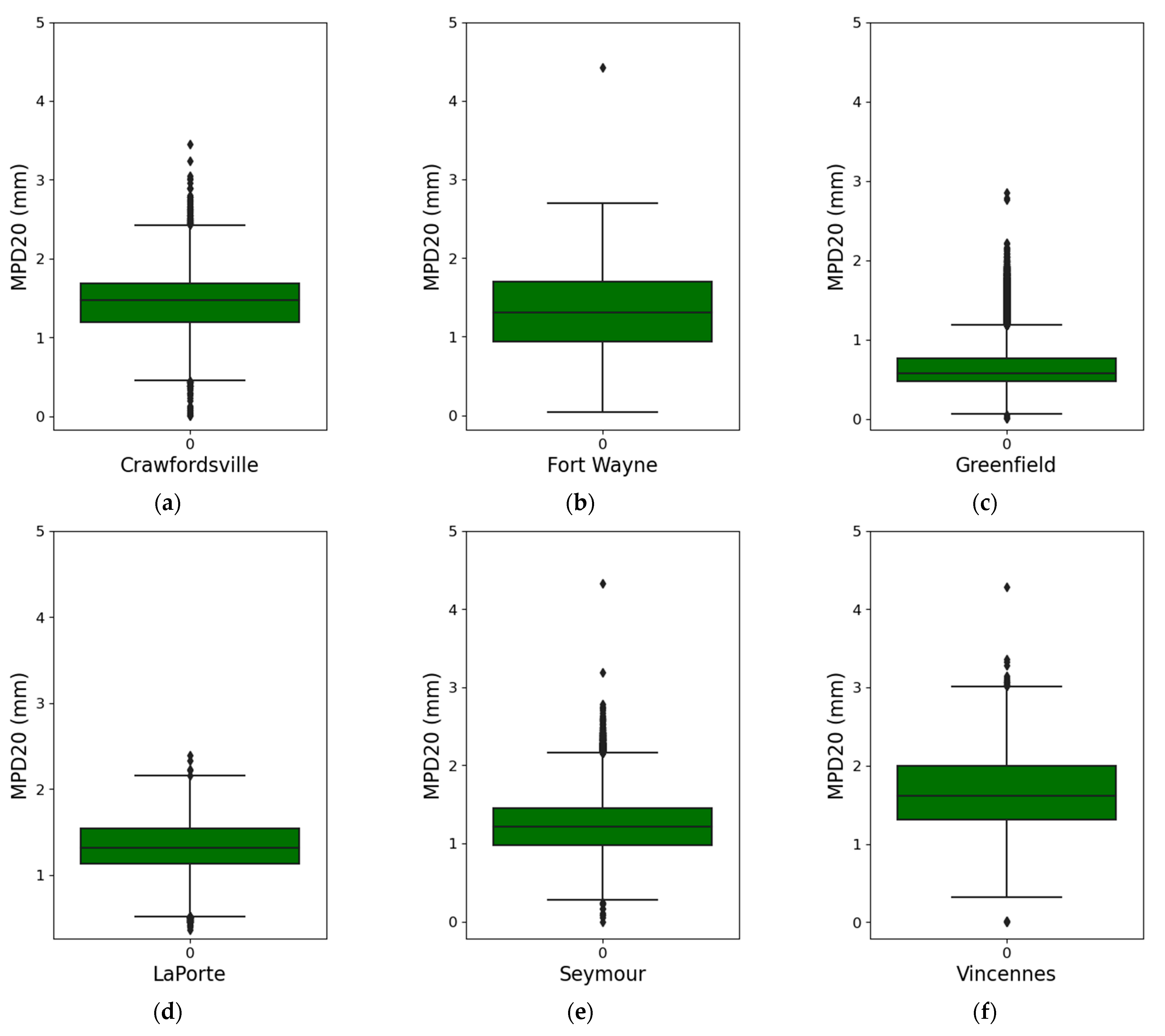
Due to regional variations in the utilization of aggregates and asphalt emulsions, the distributions of MPD₂₀ values across these regions exhibited disparities. Figure 2 presents box and whisker plots delineating the MPD₂₀ values of the six districts. A box and whisker plot is a conventional method of visually representing data distribution based on a five-number summary: the minimum, first quartile, median, third quartile, and maximum values. As shown in Figure 2, barring Greenfield and Vincennes, the quartiles at 25th, 50th, and 75th percentiles for the MPD₂₀ values across the other four districts predominantly converged around values of 1, 1.3, and 1.5 mm, respectively. Despite Greenfield and Vincennes utilizing identical asphalt emulsion and aggregate types, AE-90S and SC 11, respectively, there was a marked discrepancy in the MPD of chip seals between these two regions. Greenfield exhibited a reduced range with its 75th percentile of MPD₂₀ values being less than 0.76 mm, while Vincennes presented relatively elevated MPD₂₀ values, wherein 97.5% exceeded 0.77 mm. Differences in MPD₂₀ distributions between Vincennes and Greenfield could be attributed to multiple factors. First, the SC 11 specification allows 75–95% aggregate passage through the 9.5 mm sieve, indicating potential size variations. For instance, a higher proportion of the aggregate applied in Vincennes might be closer to 9.5 mm in size, while that in Greenfield might lean towards smaller particles, impacting the resultant MPD. Second, AE-90S, being a medium-setting emulsion, requires appropriate application and setting time. Premature traffic exposure can hinder aggregate embedding, influencing the MPD. Third, the quantity of binder, as well as the construction process and technology, can also influence the surface texture of chip seal. Finally, early and heavy traffic can further stress the aggregate, potentially affecting the MPD. The observed variability in MPD₂₀ distributions across districts underscored the imperative to conduct distinct anomaly detection tailored to each region.

In the construction of the DBSCAN-Isolation Forest model tailored for the six specific districts—Crawfordsville, Fort Wayne, Greenfield, Laporte, Seymour, and Vincennes—the hyperparameters ε and minPts within the DBSCAN component were fine-tuned. The resultant parameters for each district were as follows: Crawfordsville (0.1, 5), Fort Wayne (0.1, 2), Greenfield (0.3, 2), Laporte (0.3, 2), Seymour (0.1, 10), and Vincennes (0.3, 2), respectively. For the Isolation Forests across all districts, the parameters for ‘contamination’ and ‘number of trees’ were set to: Crawfordsville (0.1, 150), Fort Wayne (0.15, 150), Greenfield (0.1, 100), Laporte (0.15, 150), Seymour (0.1, 100), and Vincennes (0.15, 150), respectively. Figure 3 portrays the distributions of both normal data and outliers of each district. The horizontal axis represents MPD₂₀ values. The vertical axis delineates the frequency, signifying the recurrence of specific intervals of MPD₂₀ values within the given dataset. MPD₂₀ values within the normal range are delineated in blue, while those identified as outliers are highlighted in green. This visualization underscored the capability of the utilized algorithm to discern extremely high or low MPD₂₀ values as outliers, contingent on each district’s unique data characteristics. In practice, excessively high or low MPD₂₀ values can either influence ride quality or result in decreased friction. The typical MPD₂₀ values for each district, rounded to one decimal place, are showcased in

Table 4. The span of acceptable MPD₂₀ values of each district.

District	Min. MPD20 Value (mm)	Max. MPD20 Value (mm)
Crawfordsville	0.9	1.9
Fort Wayne	0.6	2.1
Greenfield	0.3	1.3
LaPorte	1.0	1.7
Seymour	0.6	1.9
Vincennes	1.0	2.3

. An MPD₂₀ or MSD value that deviated from its district’s typical range suggested that it was an outlier.

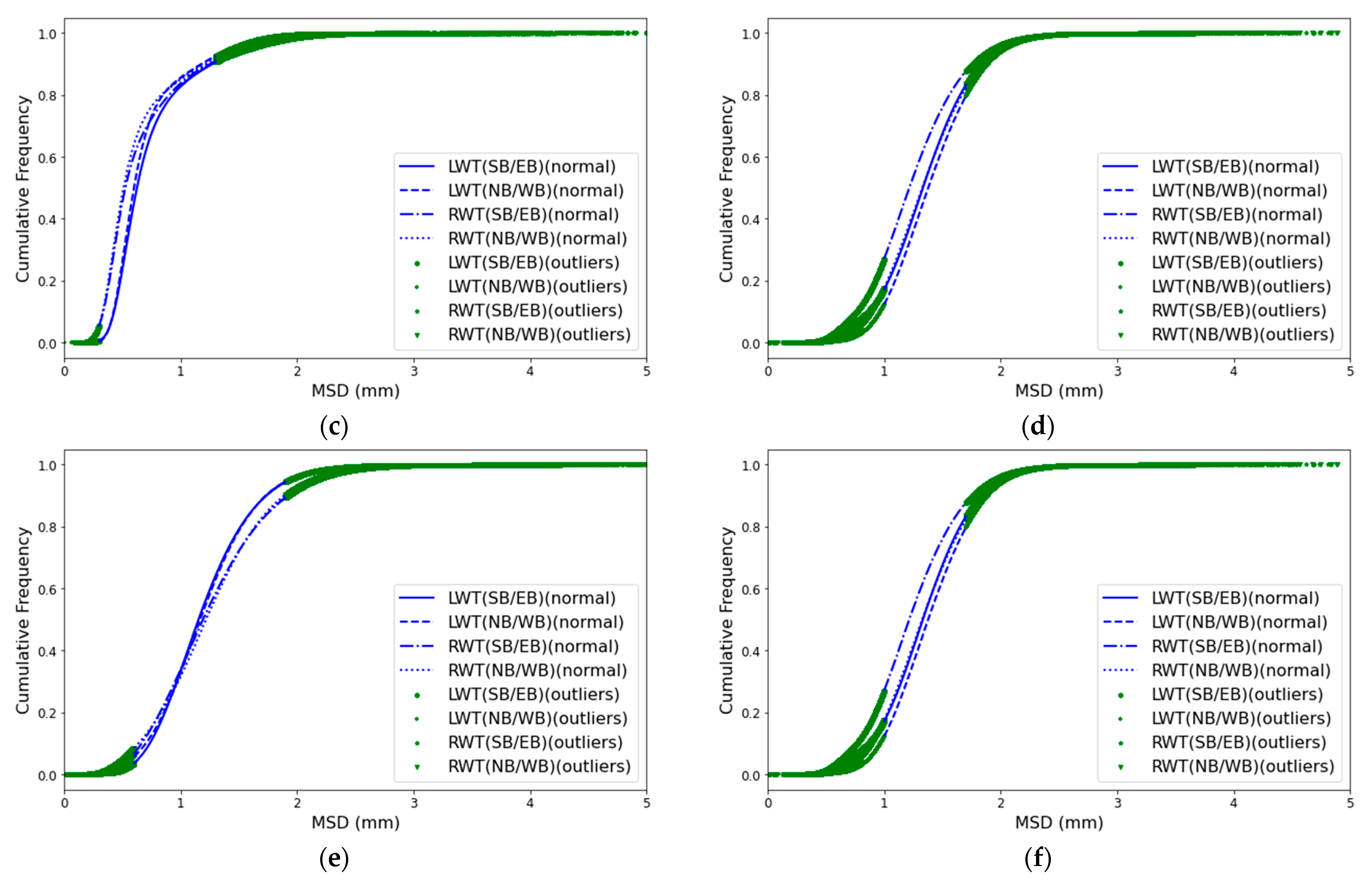
In Figure 4, the cumulative frequency distribution (CFD) is depicted, showcasing both the normal and outlier values of each district. This distribution was further stratified by wheel track and direction. The CFD provides a cumulative frequency for each category within a dataset. This approach offered a simplified visualization for the large texture datasets, making it easier to identify subtle variations in the texture measurement distribution. In this study, CFDs were utilized to analyze variations between MSD values in the right and left wheel paths in both directions. On the CFD graph, the horizontal axis denotes MSD (mm), while the vertical axis showcases the cumulative frequency. A shift to the right on this graph indicated an increase in texture depth. Post anomaly detection, the CFDs of each region revealed data retention between 60% and 90%. Excluding the Crawfordsville, Fort Wayne, and LaPorte districts, the CFDs from other regions demonstrated consistent patterns between the left wheel tracks in both directions and the right wheel tracks in both directions. However, a slight divergence was observed between the CFDs of the left and right wheel tracks. In the case of the Crawfordsville and LaPorte districts, a distinct disparity was noted in the CFDs of the right wheel tracks in both directions. For Fort Wayne, a disparity was observed in the CFDs of the left wheel tracks in both directions. Notably, the CFDs of different wheel tracks largely overlapped in the same district across varying directions, suggesting analogous patterns in data distribution. As a result, subsequent analyses in this study separately addressed the quality control of the chip seal projects from the perspective of the left and right wheel tracks.

5.2. Quality Control

The quality control process consisted of two steps. First, the outlier percentage threshold for each one-mile road segment per wheel track was established. Second, the maximum acceptable proportion of unqualified one-mile wheel track segments within the overall scope of the chip seal project’s quality acceptance was determined.

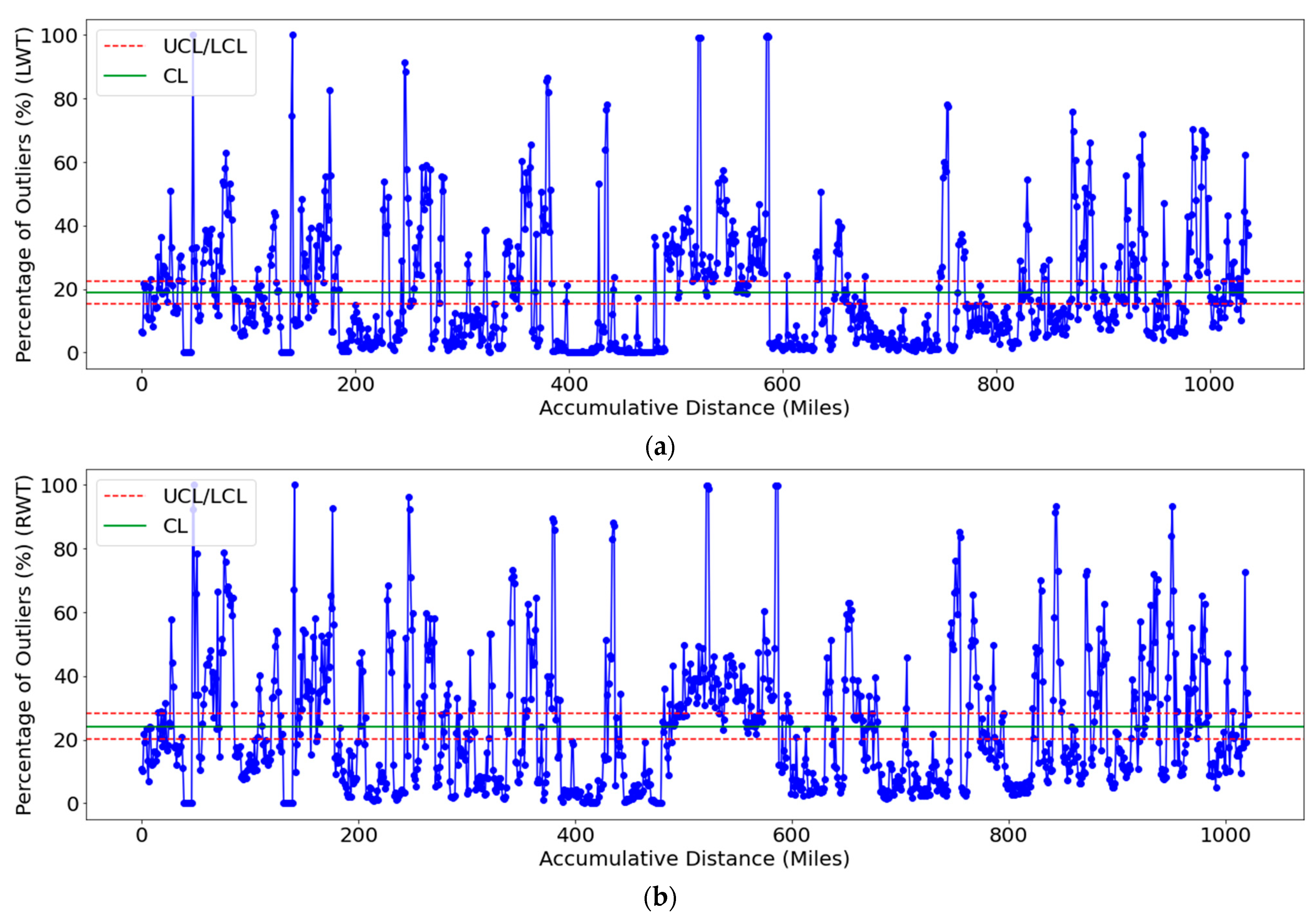
For the first stage of quality control, a dataset detailing the outlier percentage of each one-mile segment was constructed from the anomaly detection results. The dataset comprised 2059 data entries, with 1037 representing outlier percentages for the left wheel tracks and 1022 for the right wheel tracks. According to the previous analysis, one-way ANOVA was employed to determine whether there existed a significant difference between the left and right wheel track data. If the analysis yielded no statistically significant differentiation between the two datasets, they would be consolidated for subsequent evaluation; otherwise, they remained segregated. At a significance level of 0.05 for the ANOVA test, the resulting p-value was 3.27 × 10⁻⁹, which was considerably below the stipulated threshold. This underscored a pronounced difference between the outlier percentages of the right and left wheel tracks. This could be attributed to inherent variability in construction procedures. Disproportionate rolling during the construction phase and suboptimal application techniques may contribute to the observed disparities. As such, combining the two groups of data was inadvisable. Each of the two data groups was analyzed separately in the preliminary quality control procedure. Figure 5 depicts the P-charts for both the left and right wheel tracks. The horizontal axis denotes the cumulative distance, derived from the aggregated distances of individual projects. The vertical axis signifies the percentage of outliers. In Figure 5a,b, three distinct lines are present. The red dashed lines represent the upper and lower control limits. These demarcations aided in assessing the process variability. Data points lying beyond these boundaries indicated potential deviations from the expected process control. The solid green line delineates the center line, signifying the mean value of the entire dataset under examination. Despite the ANOVA results indicating significant differences between the outlier percentages of the left and right wheel tracks, Figure 5a,b revealed that the upper control limit was approximately 25%, while the lower control limit was around 18%. The results were interpreted as follows: for the one-mile segments of both the left and right wheel tracks, an outlier percentage below 18% represented exceptional chip seal performance on the designated road section. A value between 18% and 25% signified that chip seal quality on the segment was within acceptable limits. However, an outlier percentage that exceeded 25% pointed to subpar chip seal quality for that specific road segment. Therefore, the threshold for the outlier percentage of the one-mile wheel track was established at 25%.

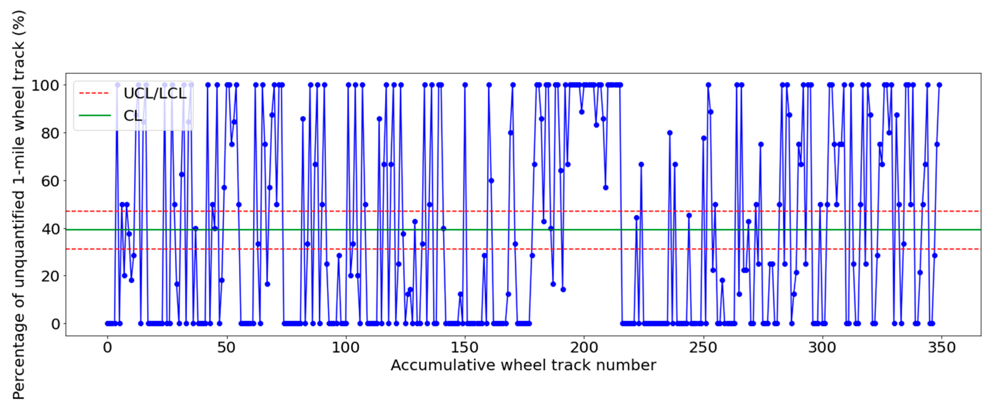
The subsequent stage in the quality control process was determining the acceptable upper limit for the unqualified one-mile wheel track rate within a chip seal project. This dataset was formed by calculating the unqualified rate for one-mile wheel tracks across all lanes and directions within a chip seal project. A “qualified” wheel track was one with a one-mile outlier percentage below 25%. In total, 350 sets of data were collected. This dataset encompassed the percentages of unqualified one-mile wheel tracks, derived from the one-mile outlier percentages for wheel tracks in both directions. Additional data points included the road name, year of chip seal project completion, and district. Figure 6 presents the P-chart employed to ascertain the threshold of the unqualified one-mile wheel track rate, serving as a metric to judge the quality of chip seal projects. The lower control limit was set as approximately 30%, indicating that projects below this line had fewer than 30% of their one-mile wheel tracks deemed unqualified. Conversely, the upper control limit, established at 50%, signified that projects exceeding this benchmark had more than 50% of their one-mile wheel tracks deemed unqualified. In evaluating the quality acceptance of a project, the performance of each wheel track must be considered. From the results, it could be deduced that a project in which fewer than 30% of its one-mile wheel tracks were deemed unqualified was of good quality. Projects with an unqualified rate between 30% and 50% for their wheel tracks were deemed acceptable, with the upper threshold of acceptability set at 50%. Any project with an unqualified one-mile wheel track rate exceeding this limit was categorized as unsatisfactory, necessitating additional assessment and scrutiny.

5.3. Validation

To validate the efficacy of the proposed anomaly detection and quality control methodology, four chip seal sections (see

Table 5. Percentages of outliers and corresponding friction numbers of designated roadways.

District	Validation Section	% of MSD < the Min. MPD20 Threshold	% of MSD > the Max. MPD20 Threshold	Overall MPD (mm)	Friction Number *
Fort Wayne	Section 1	0.4%	41.3%	2.14	59.0/61.0
Fort Wayne	Section 2	25.4%	0.3%	0.57	12.3/19.1
Seymour	Section 3	41.8%	0.1%	0.66	12.8/11.0
Vincennes	Section 4	1.4%	46.3%	2.25	60.3/58.4

* Northbound/Southbound.

) from three different districts were selected for field inspection and friction testing. These chip seal sections were identified as problematic in the preceding section. Examination of each wheel track’s characteristics in the projects revealed the following:

• In Section 1, a predominant portion of MSD outliers exceeded Fort Wayne’s 2.1 mm threshold. Notably, 97.5% of outliers in the northbound lane surpassed this limit across all wheel tracks. In the southbound lane, approximately 97.5% of outliers in the left wheel track and 95% in the right wheel track exceeded the 2.1 mm threshold. The above suggested that the surface texture may be very rough.
• In Section 2, over 95% of MSD outliers fell below the 0.6 mm threshold, encompassing all directions and tracks, which indicated a possible slippery surface.
• In Section 3, the 97.5th percentile of outliers for each wheel track fell below Seymour’s 0.6 mm mark, implying a potentially slippery surface.
• In Section 4, the 2.5th percentile of MSD outliers for each wheel track exceeded 2.3 mm, indicating a surface with a rough texture.

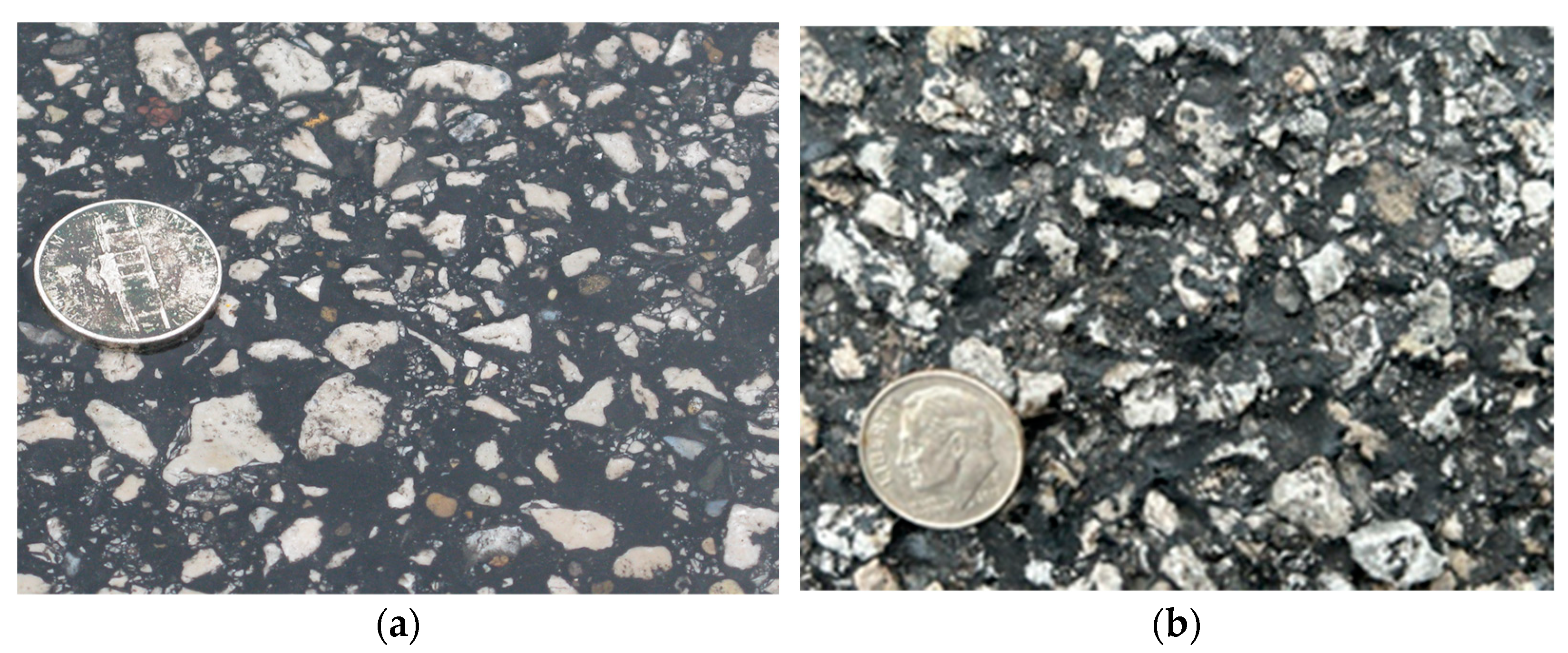
Despite unique outlier distributions across different chip seal projects, the wheel tracks in the same direction within a single project exhibited uniform characteristics. Subsequent analyses combined outliers from all four wheel tracks, focusing on the associated road section’s friction. This process aimed to further validate the proposed quality control methodology’s efficacy. Table 5 displays the percentages of outliers (larger than the maximum threshold values and lower than the minimum threshold values of a specific district) and friction measurements of the four sections. Based on the table, sections 1, 3, and 4 exhibited substantial outlier proportions, predominantly over 40%. Among them, sections 1 and 4 notably surpassed the upper 20 m MPD threshold of the corresponding districts. On the other hand, sections 2 and 3 exhibited a pronounced percentage of outliers below the minimum 20 m MPD threshold of their districts. Table 5 also presents the overall MPD values for each section, calculated as the average of all recorded MSD values within the respective section. These overall MPD values tended to approach the threshold distinguishing normal and abnormal data. However, the friction numbers measured by the LWST resonated more with the outcomes of the quality control procedure introduced in this study than with the overall MPD values. As shown in Table 5, the chip seals in sections 1 and 4 demonstrated remarkably high friction. In contrast, the chip seals in sections 2 and 3 experienced very low friction. These observations underscored the comprehensive superiority of the proposed method over previous research [13,21,40]. Further field visual inspection revealed chip seal surfaces with both very low and very high friction, as depicted in Figure 7. Evidently, both field inspections and friction measurements aligned closely with the results generated by the proposed methodology.

6. Conclusions

Excess aggregate loss and bleeding in chip seal construction can undermine its durability and functional performance, leading to potential slipperiness or compromised ride quality. The quality control of chip seals is integral to maintaining the durability, performance, and longevity of road surfaces. Regrettably, the extant literature offers limited insight into the quantification of quality control processes in chip seal construction. This research presents a streamlined quantitative approach for chip seal quality control by using both a hybrid machine learning model and the proportion control chart method. Millions of MSD data were collected using the vehicle-based texture test system, equipped with two high-speed 100 kHz point lasers, across six districts in Indiana. These data were then utilized to derive the MPD and one-mile wheel track outlier percentage datasets.

A DBSCAN-Isolation Forest model was first established to identify anomalous MPD₂₀ values for each district utilizing the MPD dataset. The normal MPD₂₀ ranges of the six districts were delineated as follows: Crawfordsville [0.9 mm, 1.9 mm], Fort Wayne [0.6 mm, 2.1 mm], Greenfield [0.3 mm, 1.3 mm], LaPorte [1.0 mm, 1.7 mm], Seymour [0.6 mm, 1.9 mm], and Vincennes [1.0 mm, 2.3 mm]. This model efficiently identified MPD₂₀ values deviating from the anticipated range, providing invaluable insight in an unsupervised context.

A two-step quality control procedure tailored for chip seal evaluation was subsequently proposed using the proportion control chart approach. Initially, the one-mile wheel track outlier percentage dataset was utilized to determine the acceptance value of one-mile wheel track outlier percentages. This investigation concluded that within a one-mile stretch, the outlier percentage for any wheel track should not surpass the 25% threshold. In the subsequent stage, the quality of each project was gauged using the unqualified one-mile wheel track percentage dataset. By harnessing the proportion control chart technique once more, a decisive threshold of 50% was derived. This signified that for any wheel track segment, the unqualified one-mile wheel track rate should not breach the 50% threshold. Surpassing this delineated boundary called for an intensified, detailed assessment.

To evaluate the robustness of the introduced methodology, four chip seal sections were selected. Friction numbers for these sections were measured using the LWST. Upon comprehensive examination encompassing outlier distribution, overall MPD, and field inspection, it was determined that the friction properties exhibited greater alignment with the findings of the quality control procedure delineated in the research than with the overall MPD values. Pertinently, the in situ observations consistently affirmed the conclusions derived from the advocated methodology.

Anchored to macrotexture characteristics, this research provides a preliminary evaluation standard of chip seal quality control for pavement construction practitioners. While the findings are promising, further research and validation are required. Firstly, only four chip seal sections were employed to validate the proposed method. In the future, the friction numbers of more chip seal sections will be collected and analyzed to demonstrate the effectiveness of this method. Additionally, while this research focused on macrotexture profiles captured on left and right wheel tracks, future endeavors will aim to obtain more detailed macrotexture information across entire roadways. Two potential methods are under consideration: the addition of more laser scanners to the vehicle-based texture test system and the exploration of efficient techniques for extracting comprehensive macrotexture information from continuous video data captured on roadway surfaces. As the field continues to evolve, methods such as the one introduced in this study will be paramount in ensuring both the efficiency of construction projects and the safety of those involved.

References

1. Shuler, S.; Lord, A.; Epps-Martin, A.; Hoyt, D. Manual for Emulsion-Based Chip Seals for Pavement Preservation. In NCHRP Report 680; Transportation Research Board: Washington, DC, USA, 2011. [Google Scholar] [CrossRef]
2. Wasiuddin, N.; Marshall, A.; Saltibus, N.; Saber, A.; Abadie, C.; Mohammad, L. Use of Sweep Test for Emulsion and Hot Asphalt Chip Seals: Laboratory and Field Evaluation. J. Test. Eval. 2013, 41, 289–298. Available online: https://www.astm.org/jte20120051.html (accessed on 5 September 2023). [CrossRef]
3. INDOT. Chip Sealing; Indiana Department of Transportation: Indianapolis, IN, USA. Available online: https://www.in.gov/indot/maintenance-operations/ (accessed on 9 August 2023).
4. Im, J.K.; Kim, Y.R. Performance Evaluation of Fog Seals on Chip Seals and Verification of Fog Seal Field Tests. Can. J. Civ. Eng. 2015, 42, 872–880. [Google Scholar] [CrossRef]
5. Gransberg, D.; Musharraf, Z. Analysis of Emulsion and Hot Asphalt Cement Chip Seal Performance. J. Transp. Eng. 2005, 131, 229–238. [Google Scholar] [CrossRef]
6. Buss, A.; Guirguis, M.; Gransberg, D. Chip Seal Aggregate Evaluation and Successful Roads Preservation. Constr. Build. Mater. 2018, 180, 394–404. [Google Scholar] [CrossRef]
7. Lawson, W.D.; Senadheera, S. Chip Seal Maintenance: Solutions for Bleeding and Flushed Pavement Surfaces. Transp. Res. Rec. J. Transp. Res. Board 2009, 2108, 61–68. [Google Scholar] [CrossRef]
8. Khattack, M.J.; Bhuyan, M.R. Performance Evaluation of Chip Seal Treatment on Flexible Pavements. Int. J. Pavement Res. Technol. 2023. [Google Scholar] [CrossRef]
9. Gransberg, D.; James, D. Chip Seal Best Practices. In NCHRP Synthesis 342; Transportation Research Board: Washington, DC, USA, 2005. [Google Scholar] [CrossRef]
10. Chipsealing in New Zealand; Transit New Zealand: Wellington, New Zealand, 2005.
11. Pavement Preservation Checklist Series 2: Chip Seal; Publication No. FHWA-HIF-19-02; Federal Highway Administration: Washington, DC, USA, 2019.
12. Li, S.; Shields, T.; Noureldin, S.; Jiang, Y. Field Evaluation of Surface Friction Performance of Chip Seals in Indiana. Transp. Res. Rec. 2012, 2295, 11–18. [Google Scholar] [CrossRef]
13. Notes for the Specification of Bituminous Reseal, TNZ P17; Transit New Zealand: Wellington, New Zealand, 2002.
14. Gransberg, D. Using a New Zealand Performance Specification to Evaluate U.S. Chip Seal Performance. J. Transp. Eng. 2007, 133, 688–695. [Google Scholar] [CrossRef]
15. Montoya, M.A.; Haddock, J.E.; Weiss, W.J. Quality Control Tool for Asphalt Emulsion-Based Chip Seal Curing Times. In Bearing Capacity of Roads, Railways and Airfields; CRC Press: Boca Raton, FL, USA, 2017; pp. 603–608. [Google Scholar]
16. Guirguis, M.; Buss, A. Chip Sealing Macro Texture Performance Evaluation Using Split-plot Repeated Measures. Road Mater. Pavement Des. 2021, 22, 185–199. [Google Scholar] [CrossRef]
17. Vijaykumar, A.; Martin, A.; Arambula, E. Revision and Further Validation of Surface Performance-Graded Specification for Chip Seal Binders. Transp. Res. Rec. J. Transp. Res. Board 2013, 2370, 44–52. [Google Scholar] [CrossRef]
18. Gransberg, D.D. Correlating Chip Seal Performance and Construction Methods. Transp. Res. Rec. J. Transp. Res. Board 2006, 1958, 54–58. [Google Scholar] [CrossRef]
19. Rahman, M.D.; Sarkar, M.T.A.; Elseifi, M.A.; Mayeux, G.; Cooper, S.B., III; Free, K. Short-Term Field Performance and Cost-Effectiveness of Crumb-Rubber Modified Asphalt Emulsion in Chip Seal Applications. Transp. Res. Rec. 2021, 2675, 1049–1062. [Google Scholar] [CrossRef]
20. Mamlouk, M.S.; Dosa, M. Verification of Effectiveness of Chip Seal as a Pavement Preventive Maintenance Treatment Using LTPP Data. Int. J. Pavement Eng. 2014, 15, 879–888. [Google Scholar] [CrossRef]
21. Zhao, G.; Li, S.; Jiang, Y.; Lee, J. Quality Assurance Procedures for Chip Seal Operations Using Macrotexture Metrics (Joint Transportation Research Program Publication No. FHWA/IN/JTRP2018/12); Purdue University: West Lafayette, IN, USA, 2018. [Google Scholar] [CrossRef]
22. Jordan, M.I.; Mitchell, T.M. Machine Learning: Trends, Perspectives, and Prospects. Science 2015, 349, 255–260. [Google Scholar] [CrossRef]
23. LeCun, Y.; Bengio, Y.; Hinton, G. Deep Learning. Nature 2015, 521, 436–444. Available online: https://www.nature.com/articles/nature14539 (accessed on 5 September 2023). [CrossRef] [PubMed]
24. Bishop, C.M. Pattern Recognition and Machine Learning; Springer: New York, NY, USA, 2006. [Google Scholar]
25. Doshi-Velez, F.; Kim, B. Towards a Rigorous Science of Interpretable Machine Learning. arXiv 2017, arXiv:1702.08608. [Google Scholar]
26. Goodfellow, I.; Bengio, Y.; Courville, A. Deep Learning; MIT Press: Cambridge, MA, USA, 2016. [Google Scholar]
27. Seitllari, A.; Kutay, M.E. Soft Computing Tools to Predict Progression of Percent Embedment of Aggregates in Chip Seals. Transp. Res. Rec. 2018, 2672, 32–39. [Google Scholar] [CrossRef]
28. Amarasiri, S.; Muhunthan, B. Evaluating Cracking Deterioration of Prevent Maintenance-Treated Pavements Using Machine Learning. J. Transp. Eng. Part B Pavements 2022, 148, 04022014. [Google Scholar] [CrossRef]
29. Gurganus, C.F.; Chang, S.; Ravipati, D.; Goehl, D.; Gharaibeh, N.G. Improving Chip Seal Construction Using Laser Intensity Data. J. Transp. Eng. Part B Pavements 2020, 146, 04020044. [Google Scholar] [CrossRef]
30. Henry, J.J. Evaluation of Pavement Friction Characteristics. In NCHRP Synthesis 291; Transportation Research Board: Washington, DC, USA, 2000. [Google Scholar]
31. Tobias, P.; de León Izeppi, E.; Flintsch, G.; Katicha, S.; McCarthy, R. Pavement Friction for Road Safety: Primer on Friction Measurement and Management Methods; FHWA-SA-23-007; Federal Highway Administration, Office of Safety: Washington, DC, USA, 2023. [Google Scholar]
32. ASTM E274/E274M-15; Standard Test Method for Skid Resistance of Paved Surfaces Using a Full-Scale Tire. ASTM: West Conshohocken, PA, USA, 2020.
33. ASTM E303; Standard Test Method for Measuring Surface Frictional Properties Using the British Pendulum Tester. ASTM: West Conshohocken, PA, USA, 2022.
34. ASTM E1911; Standard Test Method for Measuring Surface Frictional Properties Using the Dynamic Friction Tester. ASTM: West Conshohocken, PA, USA, 2019.
35. Kummer, H.W.; Meyer, W.E. Tentative Skid-resistance Requirements for Main Rural Highways. In NCHRP Report 37; Highway Research Board: Washington, DC, USA, 1967. [Google Scholar]
36. Li, S.; Zhu, K.Q.; Noureldin, S.; Kim, D. Pavement surface friction test using standard smooth tire: The Indiana experience. In Transportation Research Board 83rd Annual Meeting Compendium of Papers (CD-ROM); Transportation Research Board: Washington, DC, USA, 2004. [Google Scholar]
37. Li, S.; Noureldin, S.; Zhu, K.Q. Characterization of Microtexture on Typical Pavement Surfaces: A Pilot Study. In Proceedings of the Presented at 90th Annual Meeting of the Transportation Research Board, Washington, DC, USA, 23–27 January 2011. [Google Scholar]
38. ASTM E965-15; Standard Test Method for Measuring Pavement Macrotexture Depth Using a Volumetric Technique. ASTM: West Conshohocken, PA, USA, 2019.
39. ASTM E2157-15; Standard Test Method for Measuring Pavement Macrotexture Properties Using the Circular Track Meter. ASTM: West Conshohocken, PA, USA, 2019.
40. Adams, J.; Castorena, C.; Kim, Y.R. Construction quality acceptance performance-related specifications for chip seals. J. Traffic Transp. Eng. 2019, 6, 337–348. [Google Scholar] [CrossRef]
41. INDOT. Standard Specifications; Indiana Department of Transportation: Indianapolis, IN, USA, 2020.
42. Li, S.; Zhu, K.; Noureldin, S. Evaluation of friction performance of coarse aggregates and hot-mix asphalt pavements. J. Test. Eval. 2007, 35, 571–577. [Google Scholar] [CrossRef]
43. Li, S.; Noureldin, S.; Zhu, Z. Upgrading the INDOT Pavement Friction Testing Program; Publication FHWA/IN/JTRP-2003/23; Joint Transportation Research Program, Indiana Department of Transportation and Purdue University: West Lafayette, IN, USA, 2004. [Google Scholar] [CrossRef]
44. ASTM E1845-01; Standard Practice for Calculating Pavement Macrotexture Mean Profile Depth. ASTM: West Conshohocken, PA, USA, 2017.
45. Ester, M.; Kriegel, H.P.; Sander, J.; Xu, X. A density-based algorithm for discovering clusters in large spatial databases with noise. In Proceedings of the 2nd International Conference on Knowledge Discovery and Data Mining, Portland, OR, USA, 2–4 August 1996; Volume 96, pp. 226–231. [Google Scholar]
46. Pedregosa, F.; Varoquaux, G.; Gramfort, A.; Michel, V.; Thirion, B.; Grisel, O.; Blondel, M.; Prettenhofer, P.; Weiss, R.; Dubourg, V.; et al. Scikit-learn: Machine learning on Python. J. Mach. Learn. Res. 2011, 12, 2825–2830. [Google Scholar]
47. Bao, J.; Jiang, J.; Li, S. Determination of Safety-Oriented Pavement-Friction Performance Ratings at Network Level Using a Hybrid Clustering Algorithm. Lubricants 2023, 11, 275. [Google Scholar] [CrossRef]
48. Liu, F.T.; Ting, K.M.; Zhou, Z.H. Isolation Forest. In Proceedings of the 2008 Eighth IEEE International Conference on Data Mining, Pisa, Italy, 15–19 December 2008. [Google Scholar] [CrossRef]
49. Kutner, M.H.; Nachtsheim, C.J.; Neter, J.; Li, W. Applied Linear Statistical Models, 5th ed.; McGraw Hill Education Private Limited: New York, NY, USA, 2013. [Google Scholar]
50. Montgomery, D.C. Introduction to Statistical Quality Control, 6th ed.; John Wiley & Sons: Hoboken, NJ, USA, 2009. [Google Scholar]
Figure 1. Mean segment depth (MSD) measurements on an actual chip seal.
Lubricants 11 00409 g001
Figure 2. Box and whisker plots of MPD20 values. (a) MPD20 distribution of Crawfordsville; (b) MPD20 distribution of Fort Wayne; (c) MPD20 distribution of Greenfield; (d) MPD20 distribution of LaPorte; (e) MPD20 distribution of Seymour; (f) MPD20 distribution of Vincennes.
Lubricants 11 00409 g002
Figure 3. Distributions of both normal data and outliers of each district. (a) Distribution of both normal data and outliers of Crawfordsville; (b) Distribution of both normal data and outliers of Fort Wayne; (c) Distribution of both normal data and outliers of Greenfield; (d) Distribution of both normal data and outliers of LaPorte; (e) Distribution of both normal data and outliers of Seymour; (f) Distribution of both normal data and outliers of Vincennes.
Lubricants 11 00409 g003
Figure 4. CFDs of each district. (a) CFDs of Crawfordsville; (b) CFDs of Fort Wayne; (c) CFDs of Greenfield; (d) CFDs of LaPorte; (e) CFD of Seymour; (f) CFD of Vincennes. Note: LWT represents left wheel track; RWT represents right wheel track; SB denotes southbound; NB denotes northbound; EB denotes eastbound; WB denotes westbound.
Lubricants 11 00409 g004aLubricants 11 00409 g004b
Figure 5. P-charts for one-mile outlier percentage threshold determination. (a) P-chart for left wheel track outlier percentage determination; (b) P-chart for right wheel track outlier percentage determination. Note: LWT denotes left wheel track; RWT denotes right wheel track; UCL is the upper control limit; CL is the center line; LCL is the lower control limit.
Lubricants 11 00409 g005
Figure 6. P-charts for unqualified project threshold determination.
Lubricants 11 00409 g006
Figure 7. Close-up views of chip seal surfaces. (a) Slippery surface; (b) Rough surface.
Lubricants 11 00409 g007