Study on the Influence of Environmental Conditions on Road Friction Characteristics

Abstract

This study focuses on changes in the friction characteristics of paved roads under various conditions from the viewpoint of traffic safety. In general, the braking characteristics of road vehicles are examined using the μ–s characteristics of the tires. Therefore, in our research, we used three types of limited datasets and identified them using the Magic Formula proposed by Prof. Pacejka. Based on various experiments, it was shown that changes in the road surface environment, such as dry and wet conditions, significantly affect the μ–s characteristics, and this influence varies significantly depending on the pavement conditions. In this study, as the first stage of the analysis of these influences, it was clarified that the difference in the friction characteristics of wet and dry road surfaces varies significantly depending on the pavement surface, which is based on experimental results obtained using actual roads. As this variation is closely related to the safety of actual road traffic, we used a brush model, which is a dynamic model of the road surface and tires, to clarify the differences in this characteristic.

1. Introduction

1.1. Background

In road traffic, the longitudinal and lateral motions of road vehicles are significantly affected by road friction, which is closely related to vehicle safety. For example, obstacle avoidance, which significantly affects road traffic safety, can be categorized into two types: steering and braking. These two avoidance actions differ in the direction of the force generated between the tire and road surfaces; the former exerts side forces and the latter exerts braking forces. Although these two forces act in different directions, they are both dependent on the friction between the tire and road surfaces, and thus interfere with each other. An important result of the literature survey related to safety is as follows: In a report published by Pisano et al. on US highway crashes that occurred under adverse road weather conditions, as a result of traffic accident research by the US Department of Transformation Federal Highway Administration, 24% of the causes of traffic accidents on roads, including highways, were weather related. These accidents have been reported to be associated with ice, snow, wet road surfaces, and weather conditions, such as rain, sleet, fog, and snow [1]. Under such circumstances, accidents may be related to the driver’s field of vision and variations in the frictional characteristics of the road surface. Similarly, Andrey et al. conducted a study on collision accidents before and after a period of rainfall and confirmed that the collision rate increased by 70% on wet paved roads [2]. Moreover, according to a survey conducted by Motomatsu et al., the traffic accident rate has decreased to approximately one-fourth with the widespread use of high-performance pavements (permeable pavements) on expressways in Japan [3]. The effects of permeable pavements include securing stable road friction during rainy weather and improving driver visibility.

These results suggest that road traffic safety is strongly related to weather and that road surface conditions are expected to significantly affect the stability of vehicle motion. In particular, it has been shown that the road friction coefficient on an actual road changes greatly depending on the pavement material used, road surface condition, pavement structure, and tire structure [4,5,6,7].

As described above, the road surface friction changes significantly owing to changes in the environment. As a result, the lateral and longitudinal forces described above are strongly affected, and deceleration, such as in the case of emergency avoidance actions performed by drivers, has a large impact on deceleration and stopping-distance predictions. It will also have a significant impact on road safety management, such as the advanced safety of next-generation road traffic, including advanced driver assistance systems (ADAS) or autonomous driving vehicles (AD). Therefore, it is necessary to systematically measure road friction coefficients on actual roads, create a database, and construct a road friction estimation system as the next stage. Several studies on road friction estimation have been conducted, which can be categorized into direct methods using tire models and indirect methods using environmental information. Therefore, in the next section, we summarize road surface friction estimation methods.

1.2. Road Friction Estimation Method

As described above, road friction coefficient estimation methods are categorized into two types: one for directly measuring the tire force and the other for measuring indirect information, such as environmental information. The estimation is performed based on these results [8].

In case of the “indirect method”, a large amount of surface characteristic data of the road surface is accumulated using related sensing (road cameras, laser scanners, optical sensors, acoustic sensors, etc.), which is highly correlated with the friction force between the tire and road surface. However, as a single source of information cannot ensure sufficient estimation reliability, multiple sensors were used for the estimation. Therefore, regression model construction, machine learning, and deep learning are used based on the obtained data [9,10,11]. This type of indirect methods utilize the database described in the previous section, which we will construct after this research; however, we have conducted such research on a trial basis in the past. In this study, we propose a road surface friction coefficient estimation system based on analytical image results obtained using optical sensors, on-board cameras, and a laser radar sensor. The measurements obtained using an optical sensor are based on the principle that each road surface condition has a specific value because the main contributing component for incident light is lower than the amount of the diffuse reflection component in the reflectance on the road surface (hereafter called the albedo value). As a specific method, the main sensor is a laser radar that measures the road in front of the vehicle with high resolution, and the road surface image processing result and albedo value are compensated [9]. Furthermore, in addition to the road-surface image processing results and albedo values, measurements were also obtained using a temperature sensor. The road surface friction coefficient was estimated via inference using fuzzy logic based on the road surface measurement results, and sensor fusion was performed to compensate for each sensor’s shortcomings. It has been shown that a continuous road friction coefficient can be satisfactorily estimated [10]. Alonso et al. proposed a road condition classification system based on the real-time acoustic analysis of tires and road surfaces. As the acoustic footprint of the tire generated by the interaction between the tire and road surface varies depending on the surface conditions (such as dry, wet, frozen, and snowy) on the same road surface, the collected data are classified and output by the vector machine. Using the constructed algorithm, it was determined that dry–wet classification can be performed with a reliability of 88% or greater [11].

Direct methods for measurement are based on the data of the physical characteristics related to the friction of the tire and road surface using sensors such as load cells, piezoelectric sensors, wheel speeds, accelerometers, potentiometers, gyroscope sensors, and temperature sensors. For example, there is a method for estimating the permissible state of a road surface using the fluctuation state of the side-force characteristic with respect to the sideslip angle and the μ–s characteristics during braking. For example, Ise built a new friction measurement sensor as part of a doctoral dissertation and installed it inside a tire to measure friction [12]. Consequently, the proposed biaxial load sensor was installed on an actual tire, and it was confirmed that it is possible to measure the friction coefficient of the target surface with which the tire was in contact. This type of direct measurement method can lead to high measurement accuracy and has the potential to be reflected in control. Morinaga et al. proposed a system in which an acceleration sensor was attached to the inner surface of a tire, and the pattern of the road surface condition (road surface friction coefficient) was discriminated from the vibration waveform of the tire. Furthermore, time series data of the tire vibration in a predetermined frequency band were calculated using a band-pass filter based on the acquired original signal. The vibration level in the predetermined frequency band was calculated using a fast Fourier transform, and the road surface condition was calculated based on the vibration level. A running test was conducted on an actual roadway, and dry, wet, compacted snow, and frozen roads were classified according to their patterns with high accuracy. However, the pattern-matching computational load is high, and real-time measurements have not been realized to date. Additionally, the load applied to the tire cannot be measured directly, and the measurement results have not been applied to vehicle motion control [13,14]. Ari installed a wireless optical position sensor inside a tire (tread) to estimate the lateral deflection profile of a carcass and friction. The friction was estimated based on the principle that tread deformation is caused by the total force acting on the tire. A light-emitting diode (LED) was attached to the inner liner of the tire, an optical sensor and a magnetic pickup for reference position detection were attached to the rim, and the position-detection sensor measured the position (deflection) of the LED with respect to the rim. Furthermore, a timing pick-up sensor was used to detect the magnet attached to the suspension. The carcass and tread characteristics were modeled using springs and dampers. By comparing the friction force obtained using the algorithm with that obtained using the test machine, it was confirmed that the friction force can be accurately estimated within the normal operating range. However, the change in the frictional force owing to the relationship between the tire temperature and tire pressure was not considered [15].

This direct method has the potential to provide highly accurate friction characteristics and is easy to use for control purposes. However, there exists a problem that it is impossible to presume sudden changes in frictional characteristics such as partial freezing. Moreover, when this method is used, a model that accurately expresses tire characteristics is required.

1.3. Tire Characteristic Models

In this study, the modeling of tire characteristics was used to identify and analyze the μ–s characteristics that express the relationship between the road friction coefficient (μ) and slip ratio (s). Therefore, a model survey was conducted for this study.

According to Pacejika, tire models are classified into four stages, from empirical to theoretical models, such as those based on experimental data only and those comprising the use of the similarity method, simple physical models, and complex physical models [16].

A Carpet Plot is a representative experiment-based model. This model interpolates points obtained via experiments using spline functions and was sed before 1980 [17]. Nonlinear regions can be easily represented based on test data; however, it is necessary to narrow the interpolation width to improve the accuracy [18].

The special function model expresses the tire characteristics using polynomials and trigonometric functions. Although it does not dynamically express the tire behavior as in the case of the experimental data model, it is easy to use for simulations. A representative special function model is the Magic Formula (MF) proposed by Pacejka. This model is expressed by a function group consisting of trigonometric functions and polynomials, and its parameters are input information from the road surface and are obtained by identifying the functional group in the experimental data. This model can handle changes in tire stress in a nonlinear manner, as opposed to the conventional tire model that treats changes in stress with respect to the amount of tire deformation in a nonlinear manner. Furthermore, given that it is expressed using relatively simple formulas, it is widely used for vehicle motion state and tire friction estimation, such as computer-aided engineering analysis, owing to its ease of use and practicality [19,20,21]. It was also used in our identification because of its ease of use and high expressive power for tire characteristics.

Theoretical models generally represent the relationship between the tire force or moment characteristics, such as slip rate and slip angle, using mechanical models, and are used in various studies of friction forces in a longitudinal and lateral manner, such as the Fiala and brush models. The force, moment, and slip ratio generated by the tire were calculated and compared with those obtained using different tire models. Parameter tuning was performed to calculate the model parameters and friction coefficients. Typical theoretical models include the Fiala, brush, and string models. The Fiala model considers the part corresponding to rim of the tire as a rigid body, replaces the elastically deformable tube and sidewall with several equivalent springs, and comprises numerous independent tread rubbers in the circumferential direction of the tire. Given that the tire is treated as an elastic body, the model can express the stiffness during the bending of the tire and deformation when a bending moment is applied. It is assumed that the tire is diametrically uniform and that the lateral stiffness and deformation are not considered, which simplifies the calculations [22]. Additionally, the aforementioned model becomes very complicated if, in addition to the lateral forces, longitudinal forces, such as driving and braking forces, are simultaneously considered. Therefore, a “brush model” with a limited elastically deformable portion of the tread rubber attached to the ring is used. This model assumes that the tire carcass and belt are rigid bodies and that the tread portion within the contact patch consists of countless elastic bodies on the brushes. The force, longitudinal force, tire friction coefficient, and aligning moment were analytically obtained. It is possible to express tire behavior during braking and driving, and it is intuitively easy to handle; however, its nonlinear characteristics are difficult to express [23]. In 2003, Jacob et al. conducted a study based on the research trend of using a brush model. Based on preliminary studies, Jacob et al. found that the fit of the brush model is low in the low-slip region. Good agreement with the MF was realized in [24]. In 2021, Alexander et al. constructed a model that expressed the discrete friction coefficient μ by replacing it with the actual friction characteristics that depend on the tread temperature and sliding speed. By combining the above model and a thermal model as a substitute for the experimental temperature data, they obtained results that agreed with the MF, realized with measurements obtained using the test machine [25].

In a theoretical model, the extension of the formulation improved the accuracy of the simulation but also increased the complexity of the model. This increases the computational load and may be unsuitable for real-time simulations. Therefore, a simple model with few parameters that is highly consistent with the actual phenomena is desirable.

1.4. Road Friction Characteristics Measurement

In the previous section, we surveyed the characteristics and modelling of tire–road interfaces. Therefore, in this section, we survey the road surface friction measurements.

Civil engineers have long used a friction coefficient estimation method involving the use of a stationary British pendulum (BP) tester. The device measures low-speed friction and has a rubber slider attached to its pendulum tip. When the slider moves on the pavement surface, the frictional force reduces the kinetic energy of the pendulum. The dynamic friction (DF) of the tester can be estimated from the difference in pendulum height before and after the slider crosses the paved surface. Although it can be easily measured, it requires skill and is limited to lock μ estimation [26,27]. As this BP device is limited to low-speed friction characteristics, a DF tester was proposed by Abe to measure the friction characteristics according to speed [28]. These testers were developed to measure DF and were built to measure the frictional characteristics of the road surface on which they were installed; however, they were unsuitable for mobile measurements. This is due to the fact that until the 1990s, automobiles were not equipped with ABS, and sliding friction was an important piece of information, because tires can eventually lock when emergency braking is applied. Conversely, as many countries now mandate the use of ABS, it is common to use the peak μ of the μ–s diagram during emergency braking. Therefore, μ–s diagram measurements on actual road surfaces are now being performed. The friction coefficient estimation method comprises the use of a portable grip tester for movement measurement. One measurement tire of this device was connected to a sprocket and chain, and the speed of the measurement tire was always reduced at a constant rate with respect to the two main tires, such that braking was always applied, and the wheel rotation speed difference was measured. The friction coefficient was obtained by measuring the tire braking torque. Although it is possible to obtain continuous measurements while driving, it is only possible to measure one slip ratio condition. Therefore, it is used for measurements on road surfaces with stable friction characteristics, such as runways at airports. The problem with this method is that the peak μ cannot be directly measured when it is applied to ordinary roads. Zaid et al. measured the same road surface in Malaysia using a BP tester and grip tester, and they investigated their correlation to determine the application range of the BP tester, in which measurements can be made easily. As a result of the survey, a correlation of approximately 0.43 was obtained between the two measurement results in the Selangor state, but the measurement result in the Melaka state had an inverse correlation of −0.34. This result suggests that a DF index, such as the BP number (BPN), is not always as effective as information used in road vehicles [29]. Additionally, although the grip tester was fabricated to measure the braking force, commercial measurement instruments intended specifically for lateral force measurements with a fixed slip angle were also available. Moreover, bus- and trailer-type measurement instruments that can measure a wide range of lateral and longitudinal force characteristics are used in research institutes; however, they are very expensive and are used only for research purposes. Nevertheless, they are unsuitable for use in ordinary road vehicles.

In this study, to construct a road surface friction database and road surface friction estimation system in the future, we conducted research to construct a measurement system that meets these objectives [30,31,32,33].

Finally, we summarize the characteristics of the measurement system and define the braking force characteristics of road vehicles, as shown in Figure 1. In the figure, the peak μ and lock μ that we discussed so far are described.

Table 1. Features of the measurement system [31].

	Peak μ	Lock μ	μ–s Characteristics	Continuity	Velocity Dependence
Trailer tester Bus tester	〇	〇	〇	×	〇
Grip tester	△	×	×	〇	〇
BP tester	×	〇	×	×	×
DF tester	×	〇	×	×	〇

〇: measurable, △: partial measurement possible, ×: unmeasurable.

lists the characteristics that can be measured using the various road characteristic measurement systems discussed above. As can be observed from this table, no measuring system can be used to measure all the characteristics. In particular, from the viewpoint of vehicle safety, it is important to realize the continuous measurement of peak μ on ordinary roads. This method has been detailed in previous papers [30,31].

1.5. Purpose of Research

The final goal of this study is to systematically measure road friction coefficients and create a comprehensive database of environmental information and road friction. Previous studies have not adequately considered this type of investigation, and we believe that this study is worth conducting. To achieve this objective, our research group previously developed a trailer-type device capable of measuring three sets of μ–s characteristics. Using the MF, it was possible to identify the peak and locked values on the road surface under measurement. The aims of this study are as follows:

(1)

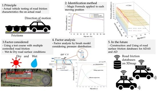
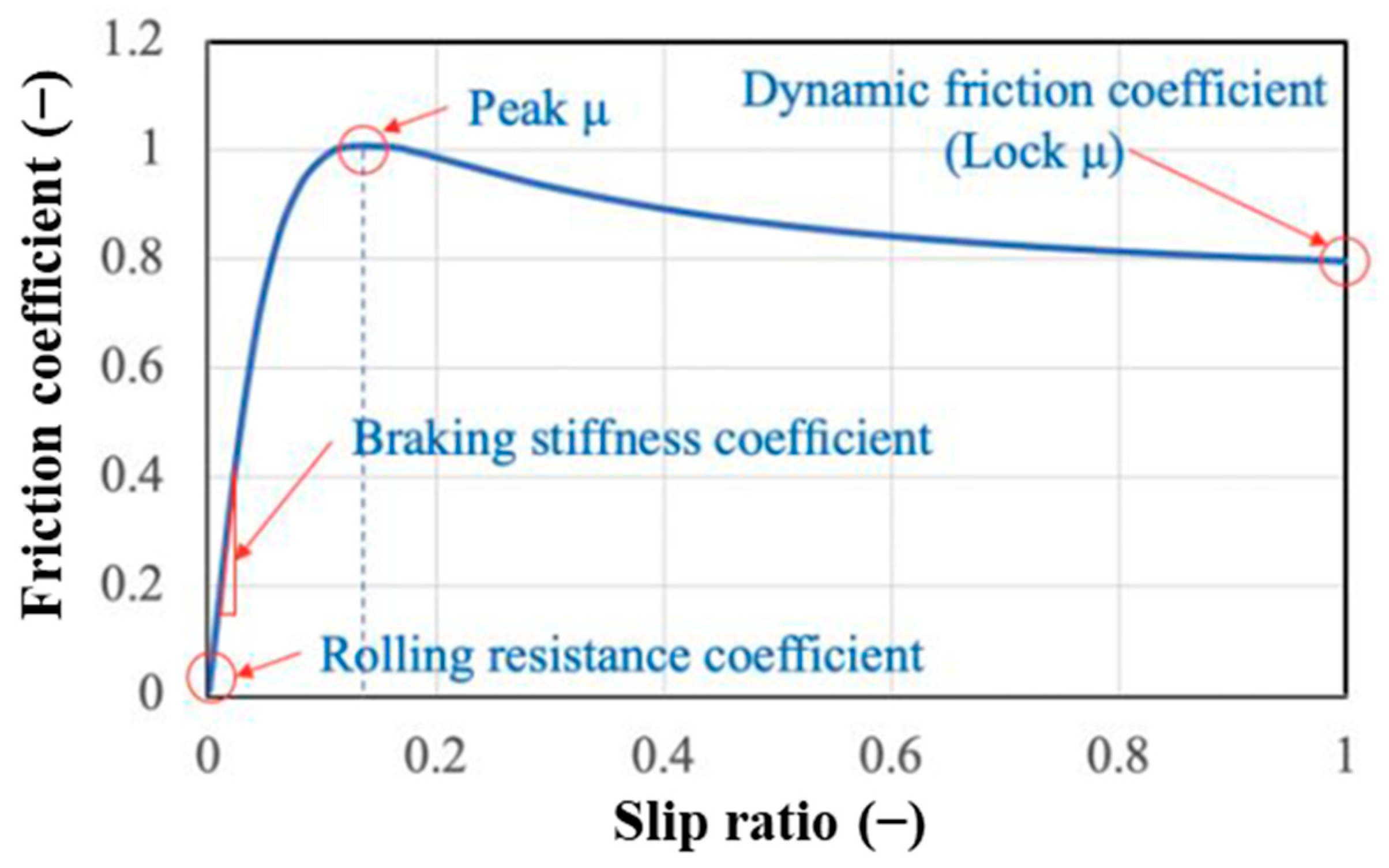
To evaluate the results of the measurements quantitatively and qualitatively on a test course, wherein the coefficient of friction on a wet surface is presented, and to better define the differences between the dry and wet surface characteristics.

(2)

To investigate and characterize the relationship between the variation of the peak μ analyzed using the brush model and the maximum static friction, DF, and tire tread stiffness.

In the following section, we present the construction of a road surface friction measurement system in line with the research objectives.

2. Constructed Measurement System

2.1. Preface

This section describes the characteristics of the measurement system used in this study. As shown in Figure 1, peak μ and shape are important for the tire characteristics during braking. However, as described above, it is necessary to identify these from the limited μ–s characteristics; such identification using a function that can express the μ–s characteristics is necessary. In addition, as shown in Table 1, the following two requirements must be met in addition to the problems to be solved:

(1)

Ability to measure friction force dependent on the running position;

(2)

Ensure continuity of data during measurement.

Figure 2 shows an example of the road friction characteristics measured during a test course. A radial tire (215/45R17) was used as the trailer-type property measuring device, and the load reaction force and internal pressure were 4 kN and 230 kPa, respectively. This is an example of a measurement performed on a wet road surface by sprinkling water from the front of a tire while it was running on a test course. In the experiment, the braking torque was gradually increased during straight running and the braking torque was released just before the tires were locked to avoid damage to the tires. On this road surface, the maximum friction coefficient was 1.156 when the slip rate was 11%, and the measurement was performed until just before the tire was locked. The friction coefficient was 0.679 when the final slip rate was 93%. Thus, rubber friction is distinct from general Coulomb friction. It is widely understood that friction characteristics vary based on the contact area, and the coefficient of friction increases as surface pressure decreases in terms of physical properties. Moreover, when modeled as Coulomb friction, the coefficient of friction can significantly exceed 1. The surface of a tire, being made of rubber, has a low Young′s modulus, which allows it to deform in accordance with the surface profile of the road. Therefore, the shearing force of the deformed rubber contributes to the braking force during braking. When rubber contacts a smooth surface, it adheres to it due to a phenomenon known as adhesion. Additionally, rubber exhibits hysteresis characteristics, which also influence friction, as documented in various tire-related technical literature [34].

Although it is necessary to express such μ–s characteristics, in this research, it is necessary to use a limited μ–s dataset for discrimination to continuously measure the road direction. Therefore, the functions used for the identification and the identification results are first presented.

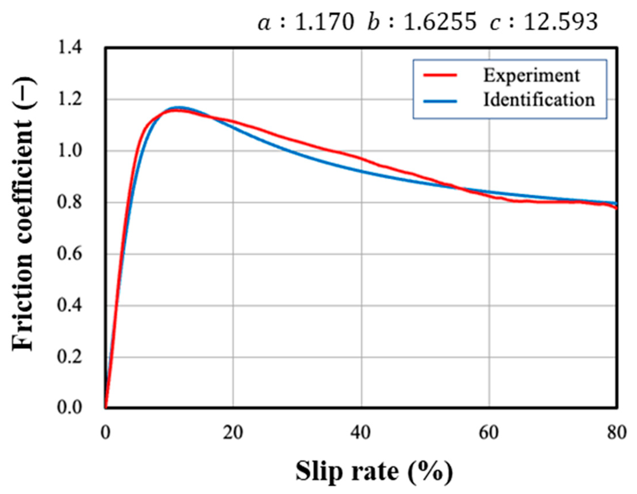
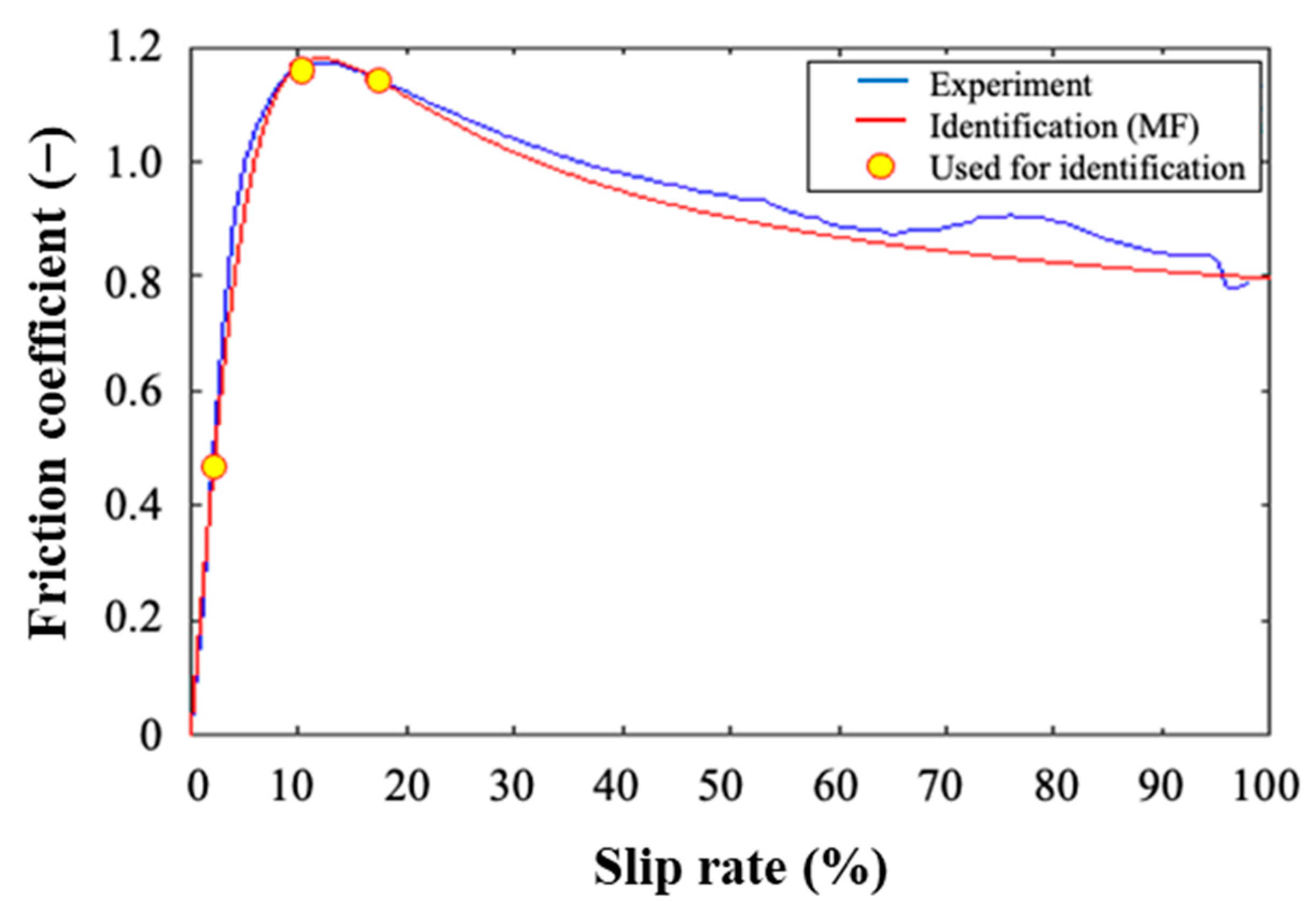
2.2. Functions and Algorithms Used for Identification

For identification, it is necessary to use a function capable of expressing the figure of μ–s characteristic. The aforementioned MF is effective for this purpose. Originally, for the MF, various subfunctions were prepared by examining methods for expressing changes, such as tire pressure fluctuation, sideslip angle, and load fluctuation. However, given that the purpose of this research was to identify the μ–s characteristics from the obtained experimental results, the use of a simple MF is considered sufficient. Therefore, the slip ratio was defined as an independent variable for this function. The slip ratio during braking is expressed as shown in Equation (1).

$$s=\frac{v-\omega r}{v}$$

(1)

Here, $s$ represents the slip ratio, $v$ represents the vehicle speed, $\omega$ represents the rotational angular velocity of the tire, and $r$ represents the tire radius. The slip ratio is nondimensional and has a value of 0 to 1 during braking, with 1 indicating a locked tire state. The slip rate is expressed as a percentage of the slip ratio, and Figure 2 shows the slip rate. Equation (2) expresses the road friction coefficient by using a simple MF.

$$\mu =asin\left\{b{tan}^{-1}\left(cs\right)\right\}+d$$

(2)

where $a$, $b$, and $c$ denote the coefficients representing the shape of the μ–s characteristics, and $d$ is the offset, which represents the rolling resistance on a horizontal road. By differentiating this function with respect to $s$, treating the differentiation result as 0, and substituting the solution for s into Equation (2), the peak $\mu$ is obtained as shown in Equation (3). However, $d$ is ignored because the rolling resistance is small.

$${\mu }_{max}=asin\left\{b{tan}^{-1}(\frac{\pi }{2b})\right\}$$

(3)

Figure 3 presents the results of identifying Figure 2 using MF. We found that this identification was sufficient.

From this result, the μ–s characteristics can be sufficiently expressed by identification performed using the MF. In the identification results presented in Figure 3, the identification was performed using the results of multipoint experiments; however, in the continuous measurement of road friction, it is necessary to estimate the μ–s characteristics by measuring the minimum set of $\mu$ and $s$. Based on this result, it is necessary to perform identification when three sets of $\mu$ and $s$ are obtained. Figure 4 presents the experimental and identification results obtained with the three-point set measurement of $\mu$ and $s$. From this result, we observe that the identification result obtained using the three points with the MF sufficiently expresses the μ–s characteristics. The measurement vehicles used for the three sets of $\mu$ and $s$ values are shown.

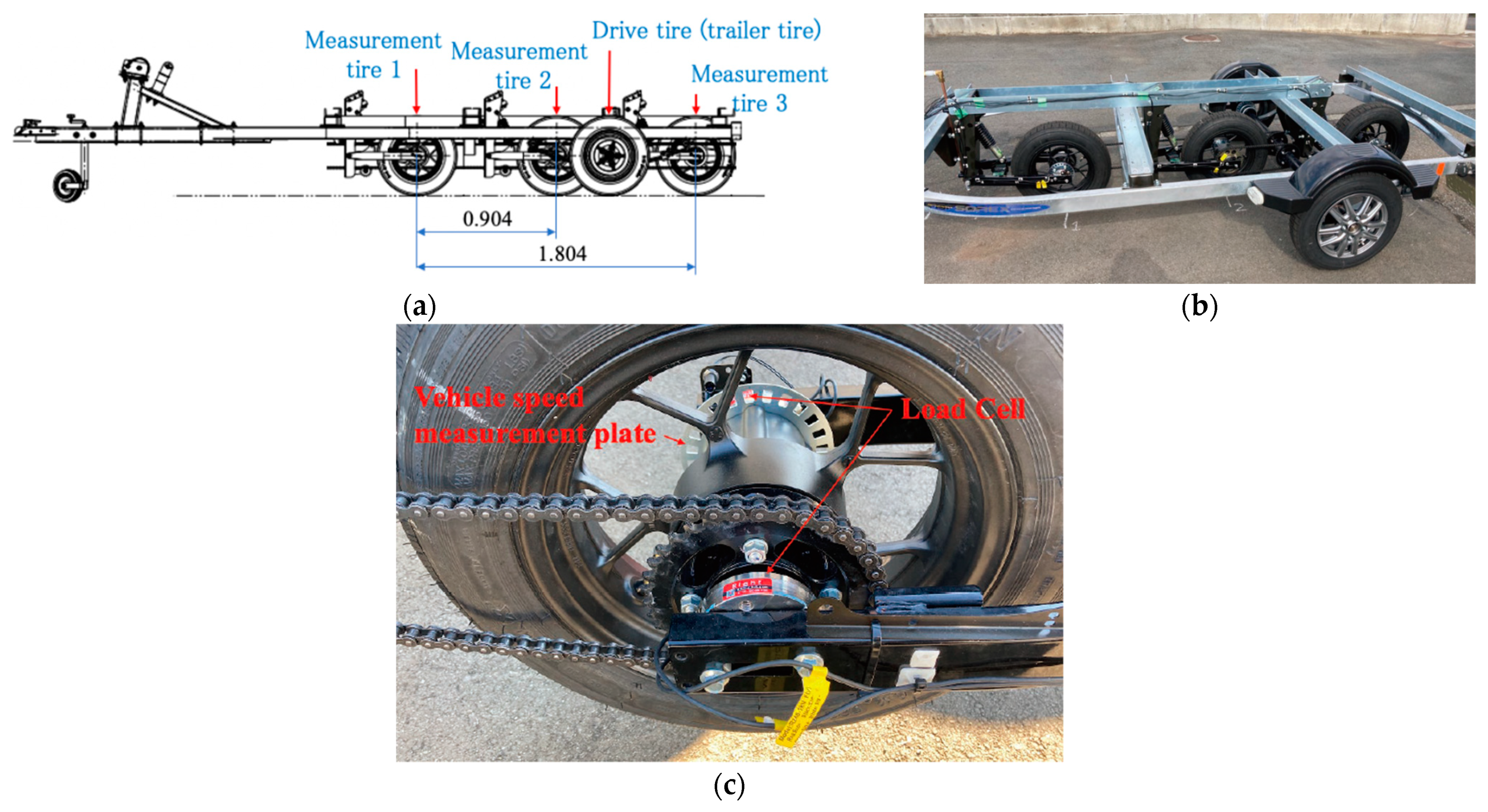
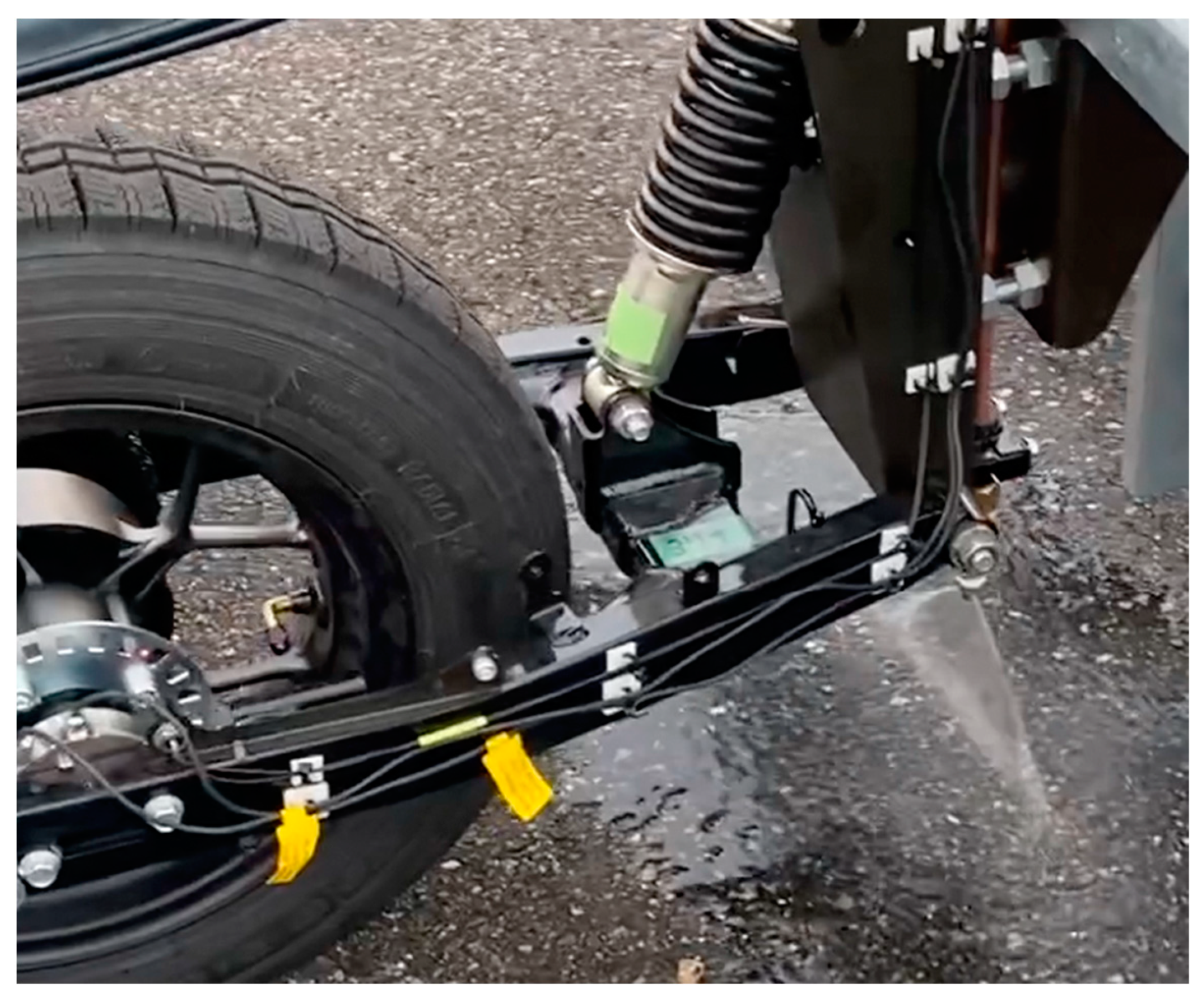
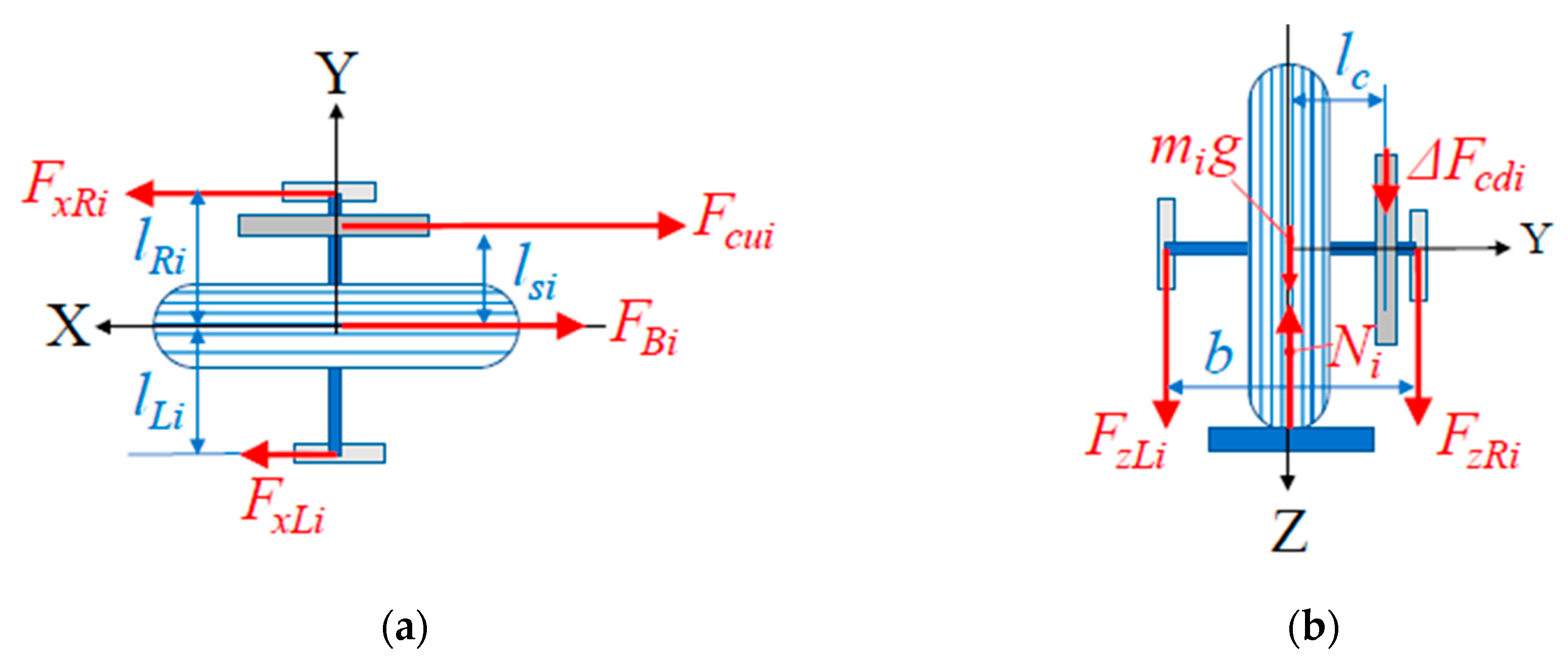
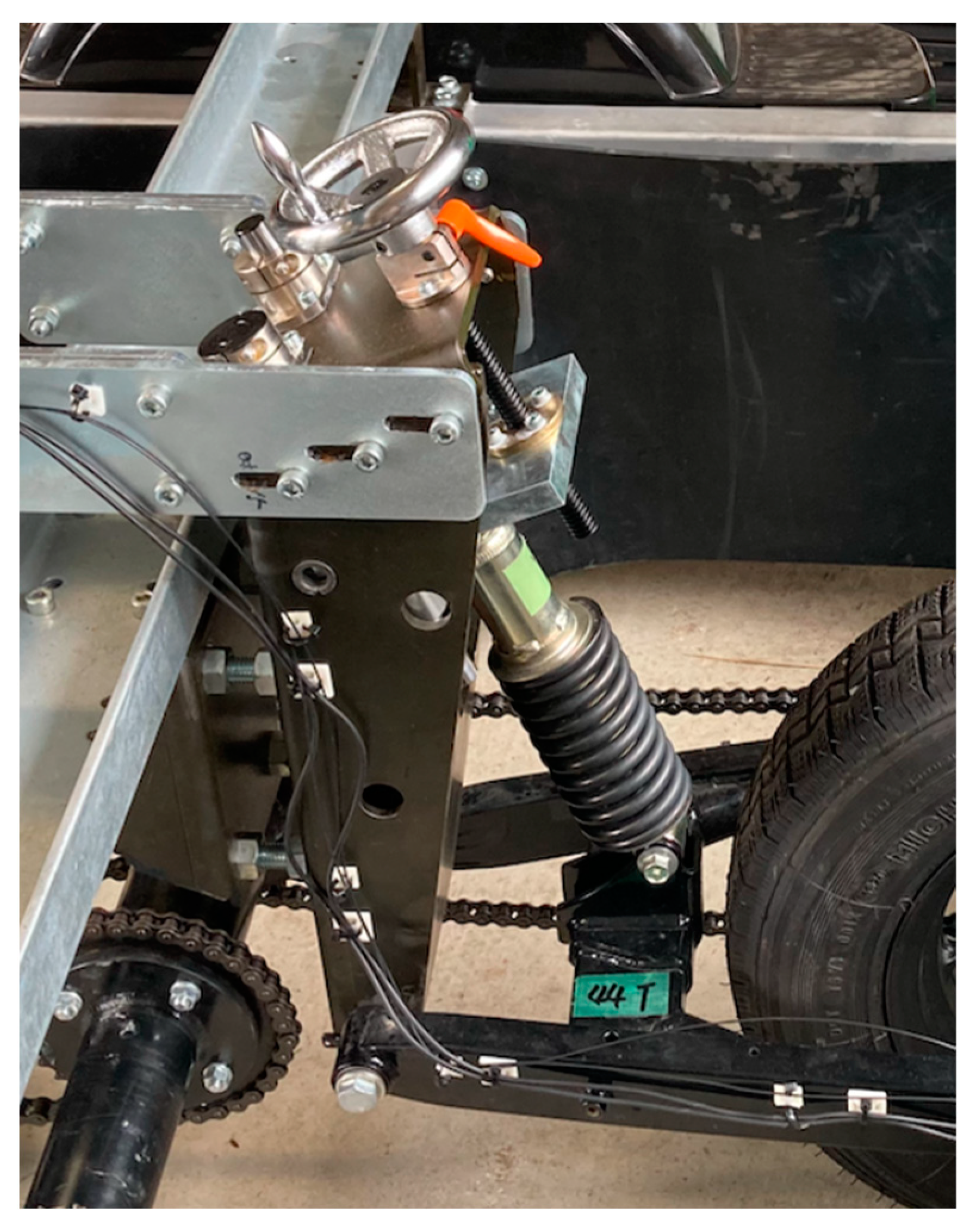
2.3. Mechanisms for Measuring Road Friction Characteristics

As shown in Figure 5, the basic structure comprises sprockets with different numbers of teeth to reduce the rotation of the driving tire (trailer main tire) and rotate the measurement tire. Consequently, the measurement tire could be operated at a constant slip ratio. In practice, three sets of tires to be measured were prepared, and three different slip ratios were obtained using sprockets with different numbers of teeth. The main tire had a negative slip ratio (driven by the measurement tires) with respect to vehicle speed, and the measurement tires had positive slip ratios. During this operation, load cells for measuring the force in two orthogonal axial directions were arranged on both sides of the axle of each tire to measure the braking force and vertical load. Each tire was equipped with a rotational pulse sensor to measure its angular velocity. From these measurement results, the slip ratios and friction coefficients of the three sets of tires were obtained.

Considering the chain length, the measurement tires were arranged with two wheels in front of the main tire and one wheel behind the main tire; to avoid chain interference, the sprocket of the second wheel was opposite to that of the other tires. Figure 6a–c presents an overview of the measurement tire arrangement of this trailer system, its photograph, and the arrangement of the load cells and speed pulse detection system, respectively. In addition, this friction characteristic measurement should comprise measurements made under dry and wet conditions. Figure 7 presents a photograph of a sprinkler installed in front of the tire to be measured.

Next, the braking and acting forces considering the chain tension are presented. Figure 8 shows the relationship between the forces acting on each tire. Here, $i$, $F_{Bi}$, and $F_{cui}$ represent the i-th set of tires, braking force, and chain tension, respectively. The force and moment balance equations for each axis are as follows:

The x-axis forces are as follows:

$$F_{xLi}+F_{xRi}=F_{Bi}+(F_{cui}+F_{cdi})cos∆{\theta }_i$$

(4)

where $∆{\theta }_i$ indicates the angle of the chain tension from the horizontal axis. The symbols for each force in the equation are presented in Figure 8.

The z-axis forces are as follows:

$$F_{zLi}+F_{zRi}+\left(F_{cui}-F_{cdi}\right)sin∆{\theta }_i+m_{i}g=N_i$$

(5)

The moment around the x-axis is as follows:

$${-l_{Li}F}_{zLi}+l_{Ri}{F}_{zRi}+l_{si}\left(F_{cui}-F_{cdi}\right)sin∆{\theta }_i=0$$

(6)

The moment around the z-axis is as follows:

$$({-l_{Li}F}_{xLi}-l_{Ri}{F}_{zRi})+l_c\left(F_{cui}+F_{cdi}\right)cos∆{\theta }_i=0$$

(7)

Using Equations (4)–(7), the braking and reaction forces were derived, as shown in Equations (8) and (9), respectively.

The braking force is as follows:

$$\begin{array}{cc}\hfill F_{Bi}=F_{xLi}+& F_{xRi}+\frac{l_{Li}{F}_{xLi}-l_{Ri}{F}_{xRi}}{l_{si}}\hfill \\ & =\left(1+\frac{l_{Li}}{l_{si}}\right)F_{xLi}+\left(1-\frac{l_{Ri}}{l_{si}}\right)F_{xRi}\hfill \end{array}$$

(8)

The reaction force is as follows:

$$N_i=\left(1+\frac{l_{Li}}{l_{si}}\right)F_{zLi}+\left(1-\frac{l_{Ri}}{l_{si}}\right)F_{zRi}+m_{i}g$$

(9)

Here, $m_{i}g$ in Equation (9) denotes the weight of the load cell at the contact point of each tire. Therefore, the friction coefficient is expressed in Equation (10) using Equations (8) and (9).

$${\mu }_i=\frac{F_{Bi}}{N_i}$$

(10)

Although the chain mounting position and chain tension direction are different between the second and third tires, the coefficient of friction for each tire was obtained using the same process.

2.4. Settings for Measurement Conditions

In the measurement of road friction characteristics, it is important to determine the type of tire to be measured and set the tire load and internal pressure that affect the tire characteristics. In particular, when measuring on ordinary roads in Japan, it is necessary to design the trailer according to the standards for lightweight trailers for towing passenger cars and to keep the total weight at less than 7.35 kN. Because the trailer has five tires, including three tires for measurement, the load on each tire should be small. In general, the friction coefficient of rubber depends on the load, and the smaller this value, the larger the friction coefficient. Considering these balances, the device was set based on the μ–s characteristics measured using a bench tire characteristic tester. A bench tester was used to conduct an internal pressure change experiment, and the peak μ was investigated. Consequently, the load for each wheel was determined to be 500 N, and the internal pressure was set to 150 kPa to set the conditions for the experiment. The set load for each measurement wheel was realized using the load adjustment mechanism installed for each measurement wheel, as shown in Figure 9. The mounting position of the suspension spring in the device is adjusted using a steering wheel.

3. Experiments on Proving Ground

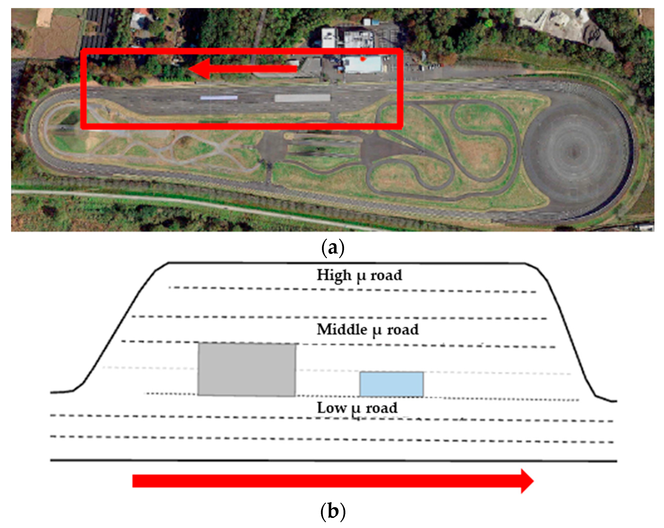
3.1. Outline of Measurement Course

The measurements were obtained at a proving ground in the Tochigi Prefecture, as shown in Figure 10a, where the friction coefficient under wet conditions is presented. To make it easier to understand the outline of the course used in the experiment, Figure 10b presents diagrams with different aspect ratios. The friction coefficients under wet conditions are as follows: high-friction coefficient road (wet friction coefficient of approximately 1.0: high-μ road), medium-friction coefficient road (wet friction coefficient of approximately 0.9: middle-μ road), and low-friction coefficient road (wet friction coefficient of approximately 0.75: low-μ road). The vehicle travels in the direction indicated by the arrows in the figure. In addition, positioning plates were placed during the course and positioning between the data points was performed using the plates.

3.2. Experimental Data

Figure 11 presents an example of the analysis results based on the data obtained via measurements. Using the road friction measuring device described in Section 2, the trailer was driven at a speed of 40 km/h on a wet surface with a relatively flat paved surface. Based on a 10 s constant-vehicle-speed section, the coefficient of friction of each tire is shown with respect to the running position. The average speed during this period was 12.3 m/s, and the travel distance was approximately 120 m. The coefficient of friction fluctuated with respect to the running position, even on the proving ground, and it appeared to be almost flat and uniform.

Next, as shown in Figure 6a, the mounting positions of the three measured tires were shifted in the fore and aft directions; hence, when performing the identification at each position, it was necessary to verify the difference in mounting positions.

This problem could be solved by interpolating the coefficient of friction for each tire distance. The measurement frequency was 100 Hz, the measurement data number was approximated to an integer using the number attached to each measurement point, and the same point was treated as the friction coefficient when passing through it. If the measurement number of the first tire is n at a vehicle speed of 40 km/h, then those of the second and third tires data record number are n + 7 and n + 15, respectively. To obtain these values, the MF approximation was used to determine the μ–s characteristics. Figure 12 presents the results of comparing the peak obtained μ and lock obtained μ values for the running position obtained from the obtained μ–s characteristics before and after the correction. The effect of the changing peak μ is almost negligible; however, if the change in the friction properties is large, the effect on lock μ can be observed. Based on this compensation method, we considered the influence of friction characteristic variation with position.

3.3. Measurement Results

For the experimental conditions, the measurement target speeds were set at 4 levels: 5, 20, 40, and 65 km/h. The peak μ and lock μ were obtained from the load cell output of each tire from the section wherein the speed became constant on using the identification method with the MF. As described in the previous section, the greatest feature of this road surface friction measurement system is its ability to continuously measure the peak μ variation with respect to positional changes. In this report, as an example, the results of a continuous measurement on a high-μ road and low-μ road when running at a speed of 65 km/h are shown. Figure 13 shows the results for dry and wet road surfaces while driving on a high-μ road. From this result, it is found that the value of the peak μ is approximately 0.4 to 0.45 lower on the wet road surface than on the dry road surface. In addition, the decrease in the friction coefficient near the running position of 45 m on the horizontal axis and the increase in the friction coefficient immediately after that exhibited the same trend, despite the difference in wet and dry conditions. In addition, the value of the peak μ of the wet condition on this road surface is approximately 1.0, but it was found that the peak μ fluctuated around 1.0, even in the results obtained using this device, and the value of the wet condition was quantitatively measured.

Figure 14 shows the measurement results for the dry and wet conditions while driving on a low-μ road. On the horizontal axis, “0” represents the beginning of the low-μ road, and the section from there to approximately 270 m is the low-μ section. In addition, from the relationship of the pavement continuity, it can be observed that the low-μ state is reached after a variable section of approximately 30 m. This result clearly appears in the wet condition. Before and after this low-μ section, the friction characteristics are almost the same as those of the high-μ road in the wet condition. When observing this low-μ section on a dry road surface, it was found that there was not much variation compared to the sections before and after this section. Therefore, even in this low-μ section, a relatively high road surface friction coefficient is secured under dry conditions; however, under wet conditions, the friction coefficient decreases rapidly, with a maximum reduction of approximately 0.6. Although there was little difference in appearance between the two road surfaces, the degree of decrease in the coefficient of friction differed significantly when the road surface became wet. It was also found that a decrease of approximately 40–50% occurred, and such a road surface database is important from the viewpoint of road traffic safety.

4. Braking Force Analysis Using Brush Model

4.1. Brush Model

In the brush model, it was assumed that the tread rubber was fixed to the tread base and that there was no interference between individual brushes. Furthermore, the contact between the brush and road surface is affected by the static friction and DF, and the ground and brush are fixed in the static friction area, which is called the adhesion region. Moreover, in DF, slippage occurs between the brush and road surface, and this area is called the sliding region.

As shown in Figure 15a, during braking ($s$ > 0), the ground displacement is greater than that of the tread base. Figure 15b shows the relationship between the time and the amount of movement. Additionally, it was assumed that there was no slippage on the contact surface.

Based on Figure 15b, the relative displacement between the road surface and the tread base is given by Equation (11).

$$∆x=\frac{(v-\omega r)}{v}x$$

(11)

Here, the first term on the right side is defined as the slip ratio $s$. Furthermore, if $k_x$ is the longitudinal rigidity of the brush at position $x$, and $b$ is the tread width, the force generated in this brush is expressed by Equation (12).

$$f_x=k_x\cdot b\cdot \Delta x\cdot dx$$

(12)

Therefore, the force generated by the brush on the entire contact surface (contact length = $l$) is given by Equation (13):

$$F_x=\int f_x={\int }_0^l{k}_{x}b\Delta xdx=k_{x}bs{\int }_0^{l}xdx=\frac{1}{2}{k}_{x}b{l}^{2}s$$

(13)

From this equation, if no slip occurs between the road surface and brush, these forces are proportional to the slip ratio, and the braking coefficient $K_B$ is given by Equation (14).

$$K_B=\frac{1}{2}{k}_{x}b{l}^2$$

(14)

From this equation, it was found that the braking force in the adhesion region is determined only by the tire conditions, such as the longitudinal rigidity of the brush, tire width, and contact length.

When examining the actual tire characteristics using a brush model, it is necessary to consider the sliding region. In order to determine this sliding region, it is necessary to consider the state at which the maximum static friction is reached according to the magnitude of the vertical load and the relative displacement $\Delta x$. For this purpose, it is necessary to assume the pressure distribution in the tire contact patch. Therefore, Equation (15), proposed by Sakai, was adopted, where $p$ is the contact pressure, $l$ is the contact length, $w$ is the contact width, $F_Z$ is the contact load, and $n$ is the shape.

$$p=\frac{n+1}{n}\frac{2^n{F}_Z}{l^{n+1}w}\left\{{\left(\frac{1}{2}\right)}^n-{\left(x-\frac{1}{2}\right)}^n\right\}$$

(15)

Figure 16 shows the shape when the value of n is changed. Furthermore, according to Sakai, $n$ = 4 is appropriate for the contact pressure distribution of radial tires; therefore, this value was adopted [34]. The ground length in this figure was standardized to 1, width to 0.4, and standardization of $F_Z$ to 1. Multiplying the surface pressure of each part by the minute area, $wdx$, provides the load that the brush bears.

$$f_{xmax}={\mu }_{i}pwdx$$

(16)

Here, ${\mu }_i$ is the maximum friction coefficient, $i$ = s is the maximum static friction ${\mu }_s$, and $i$ = D is the DF ${\mu }_D$. If the maximum displacement of the brush is ${∆x}_{max}$, from Equations (12) and (16), it is obtained using Equation (17):

$${\mu }_{i}pwdx={∆x}_{max}kwdx$$

(17)

Therefore, the maximum displacement of each brush is given by Equation (18):

$${∆x}_{max}={\mu }_i\frac{p}{k}$$

(18)

Furthermore, the displacement of the brush in the contact patch is given by Equations (19) and (11), although it varies depending on the slip ratio.

$$∆x=sx$$

(19)

Equation (20) is obtained by determining the intersection point $x_c$ of Equations (18) and (19).

$$x_c=\left(\frac{f_1}{{30\mu }_s}-\frac{{5\mu }_s}{3f_1}+\frac{2}{3}\right)l$$

(20)

Here, $f_1$ in the equation is given by Equation (21).

$$f_i=\sqrt[3]{\left(-1350abcs\right)+150\sqrt{3}\sqrt{27a^2{b}^2{c}^2{s}^2-50{\mu }_{s}abcs+25{{\mu }_s}^2}+1250{\mu }_s){{\mu }_s}^2}$$

(21)

Here, a, b, and c represent the parameters obtained by approximating the μ–s diagram using the MF. Here ${\mu }_i$ is ${\mu }_s$. Next, by multiplying Equation (19) by the spring constant and integrating it, the braking force component owing to static friction is calculated, and Equation (22) is obtained.

$$F_s=\frac{kws{x_c}^2}{2}$$

(22)

Similarly, the force generated by DF is the braking component due to DF, which is integrated from this cross-point $x_c$ to l based on the result of ${\mu }_i$ in Equation (18) being ${\mu }_D$. Subsequently, we obtain Equation (23):

$$F_D={\int }_{x_c}^l{\Delta x}_{max}kwdx=k_{x}w{f}_2$$

(23)

Here, $f_2$ in the equation is described by Equation (24)

$$f_2=\frac{{\mu }_D}{abc}\left\{-\frac{2\left(l^5-{x_c}^5\right)}{l^3}+\frac{5\left(l^4-{x_c}^4\right)}{l^2}-\frac{5\left(l^3-{x_c}^3\right)}{l}+\frac{5\left(l^2-{x_c}^2\right)}{2}\right\}$$

(24)

Therefore, the braking force for this slip ratio can be obtained by adding (23) and (24). The braking force characteristics can be calculated by changing s in the equations.

As an example, Figure 17 presents a conceptual diagram of the calculation results obtained with a contact width of 0.2 m, contact length of 0.25 m, $F_Z$ of 2.5 kN, and brush fore and aft rigidity of 8 × 106 N/m². The brush displacement with a constant slip ratio, shown in Figure 13b, is superimposed in this figure. Assuming that the slip ratio is constant and the relative speed between the road surface and tread base is constant, it increases linearly; however, when it reaches ${∆x}_{max}$, which is described as the maximum static friction, no further frictional force can be obtained, and it starts to slip. However, there exists a mixture of brushes that have reached a critical state and those that have not. For simplicity, we did not consider the comprehensive line characteristics from the maximum static friction to DF. Therefore, each brush was displaced along the green line, and the braking force was calculated from these displacements using Equation (23).

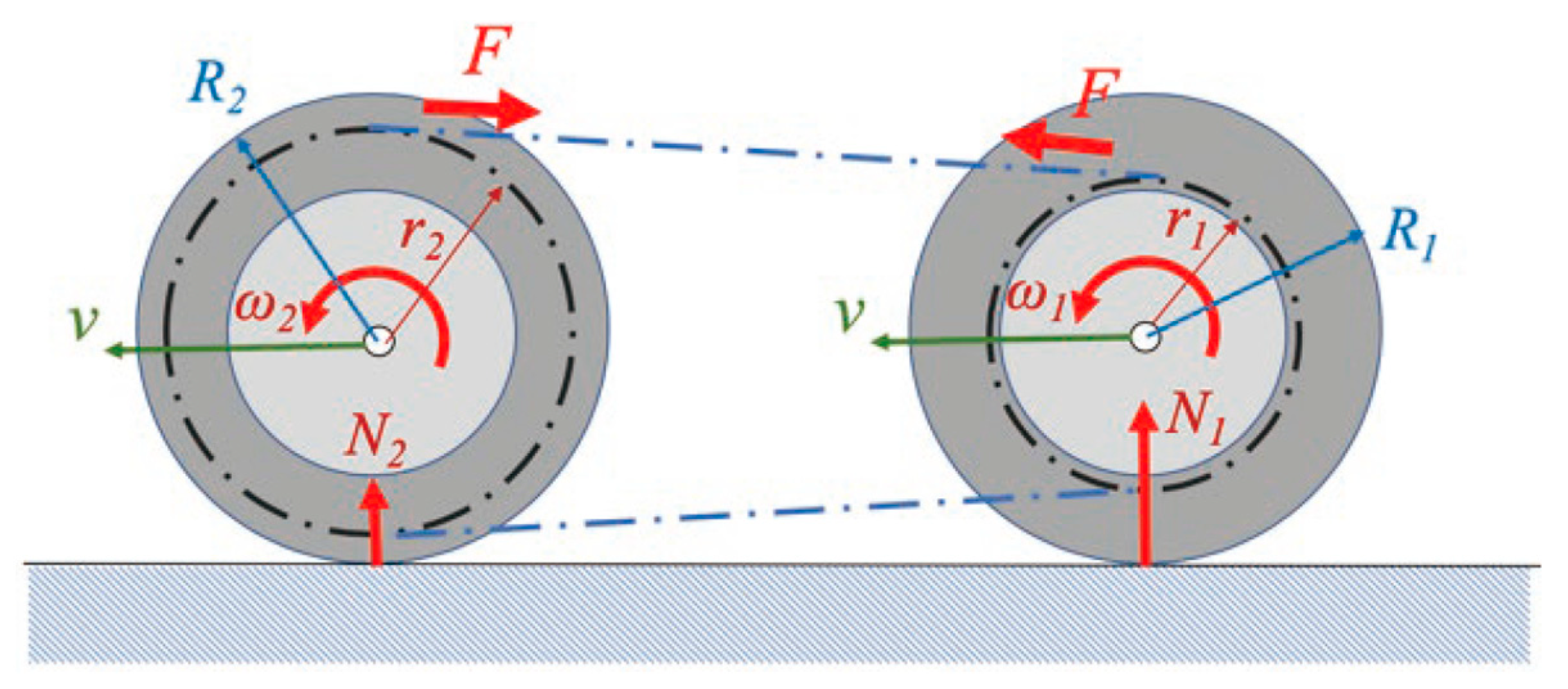
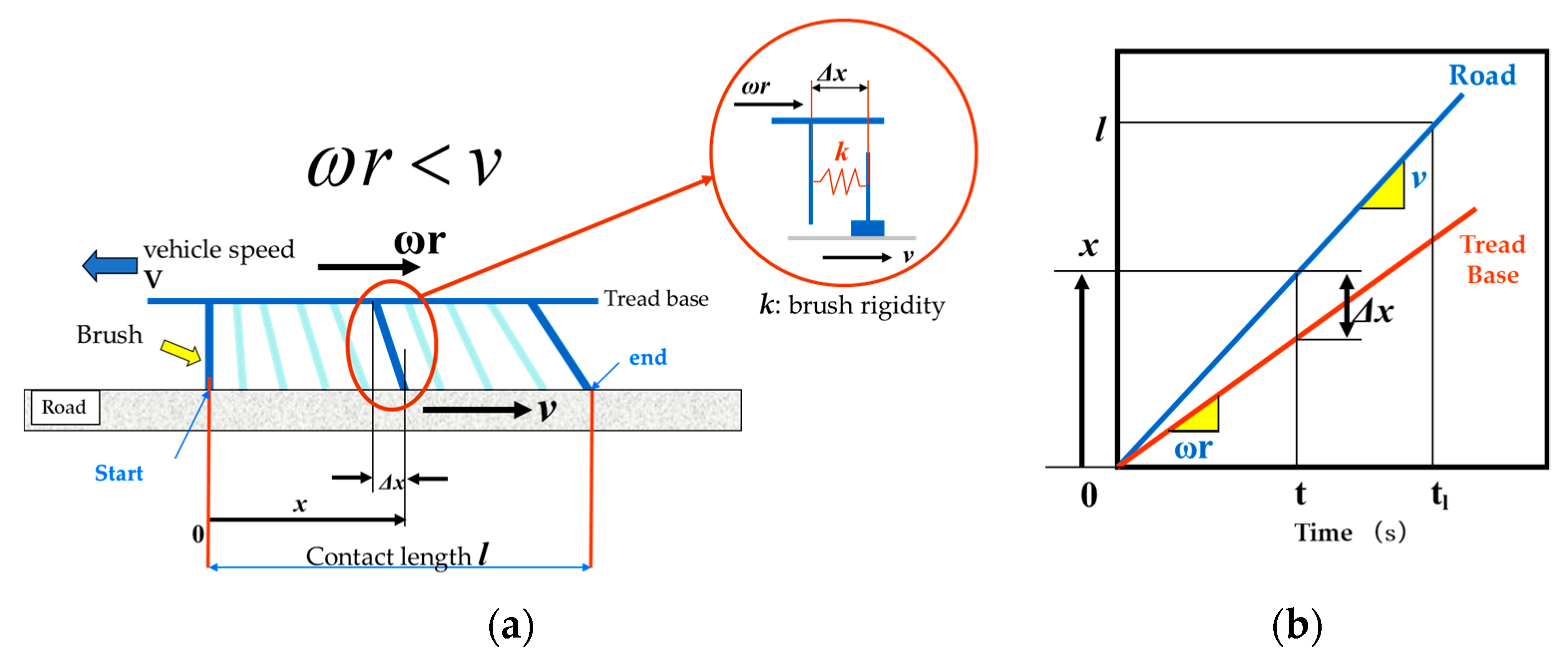
Based on these results, Figure 18 presents a comparison of the identification results obtained using the MF and those obtained using the brush model. To identify the brush model, the lock μ of the MF was ${\mu }_D$, and ${\mu }_s$ was used as a parameter. As a result, it was found that good identification can be realized with the brush model.

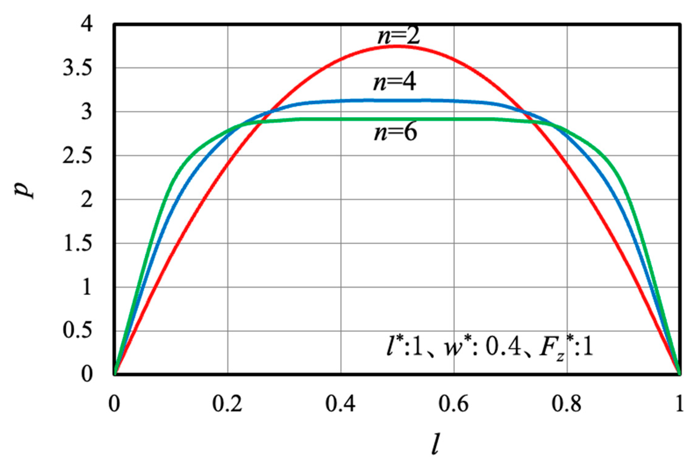
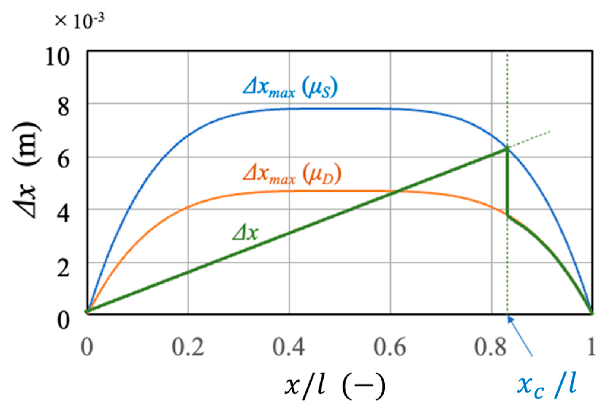
4.2. Analysis of Peak μ Position Using Brush Model

Using the brush model, it is possible to separate the components of the μ–s characteristics into adhesion and sliding regions. The analytical results are shown in Figure 19 as an example. As an example, the results were obtained by analyzing ${\mu }_s$ at 1 and ${\mu }_D$ at 0.3 and 0.5. In the analysis under these conditions, as ${\mu }_s$ is the same, the adhesion region term is the same in the two figures, but the sliding region term varies greatly. It was found that the shape of the μ–s characteristic and the peak μ value were significantly different. Therefore, it is effective to perform such a factor analysis for μ–s characteristic estimation.

The relationship between the magnitude of the peak μ and the slip ratio that produces that value is important for safety. As these values were obtained by measuring the μ–s characteristics of the road surface, their shapes could not be predicted. As a first step in predicting them, we attempted to estimate the shape of these μ–s characteristics from the relationship between ${\mu }_s$ and ${\mu }_D$. Therefore, we considered using the following new parameters:

$$\begin{gathered} n_1=\frac{{\mu }_d}{{\mu }_s} \\ {n}_2=\frac{abc}{{\mu }_s} \\ {n}_3=\frac{{\mu }_{max}}{{\mu }_s} \end{gathered}$$

(25)

Here, $n_1$ represents the ratio of ${\mu }_D$ to ${\mu }_s$, and $n_2$ represents the ratio of the rising slope of the μ–s characteristic to ${\mu }_s$. Using these as explanatory variables, the peak μ is obtained, and this value is used as the objective function as a ratio to ${\mu }_s$.

Figure 20a presents the change in $n_3$ when $n_1$ was varied from 0.1 to 0.8 and $n_2$ was varied from 1 to 6. From these results, it was found that the effect on $n_3$ is greatly influenced by the variation in $n_2$, and the influence on the slip ratio that gives the peak $\mu$ is greatly influenced by $n_1$. By conducting these verifications in greater detail, it is possible to investigate the shape and value of the μ–s characteristics. By measuring ${\mu }_s$ and ${\mu }_D$ directly, the μ–s characteristics can be estimated.

5. Conclusions

Road safety strongly depends on tire characteristics; however, the characteristics of actual roads have not yet been clarified. With the aim of providing safety-enhancing information for ADAS and AD, which are becoming popular, we developed a system for measuring road friction and constructed a prototype measurement device. In this study, we demonstrated the importance of road friction measurement according to the measurement of road position and established the necessary equipment repair and correction methods. Experiments were then conducted under various wet and dry conditions on a proving ground with specified road surface friction coefficients. It was shown that the level of reduction in the peak characteristics on wet roads varied significantly depending on the pavement and other conditions. In addition, a basic analysis for predicting future peak μ characteristics is presented using a dynamic brush model. The following conclusions were drawn:

(1)

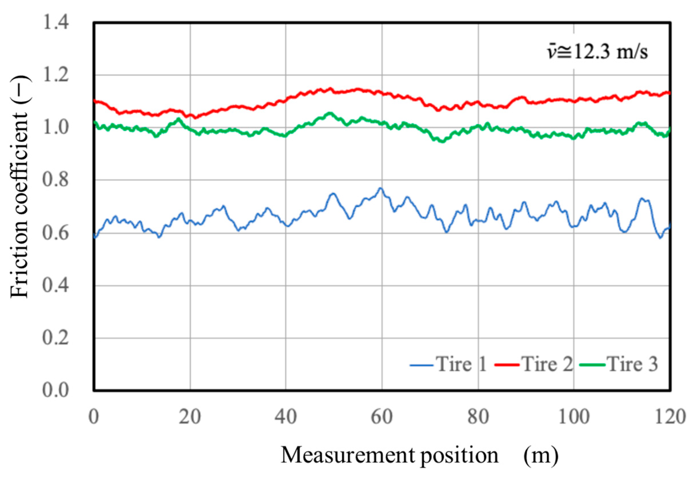
From the results of the measurements of the road surface, which appeared to be almost uniform, it was confirmed that the friction characteristics always fluctuated, and the importance of continuous measurement of the road surface friction characteristics was demonstrated.

(2)

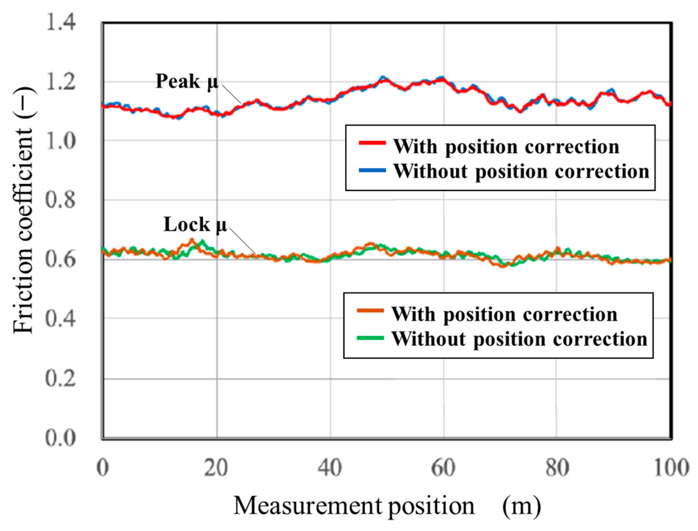
When applying a road friction coefficient measurement method that depends on the road position, the problem with this measurement system is that the mounting position of each measurement tire is offset in the fore and aft directions. Therefore, we present a method for obtaining the friction coefficient at the same road position by correcting the friction coefficient measured at each tire with respect to distance.

(3)

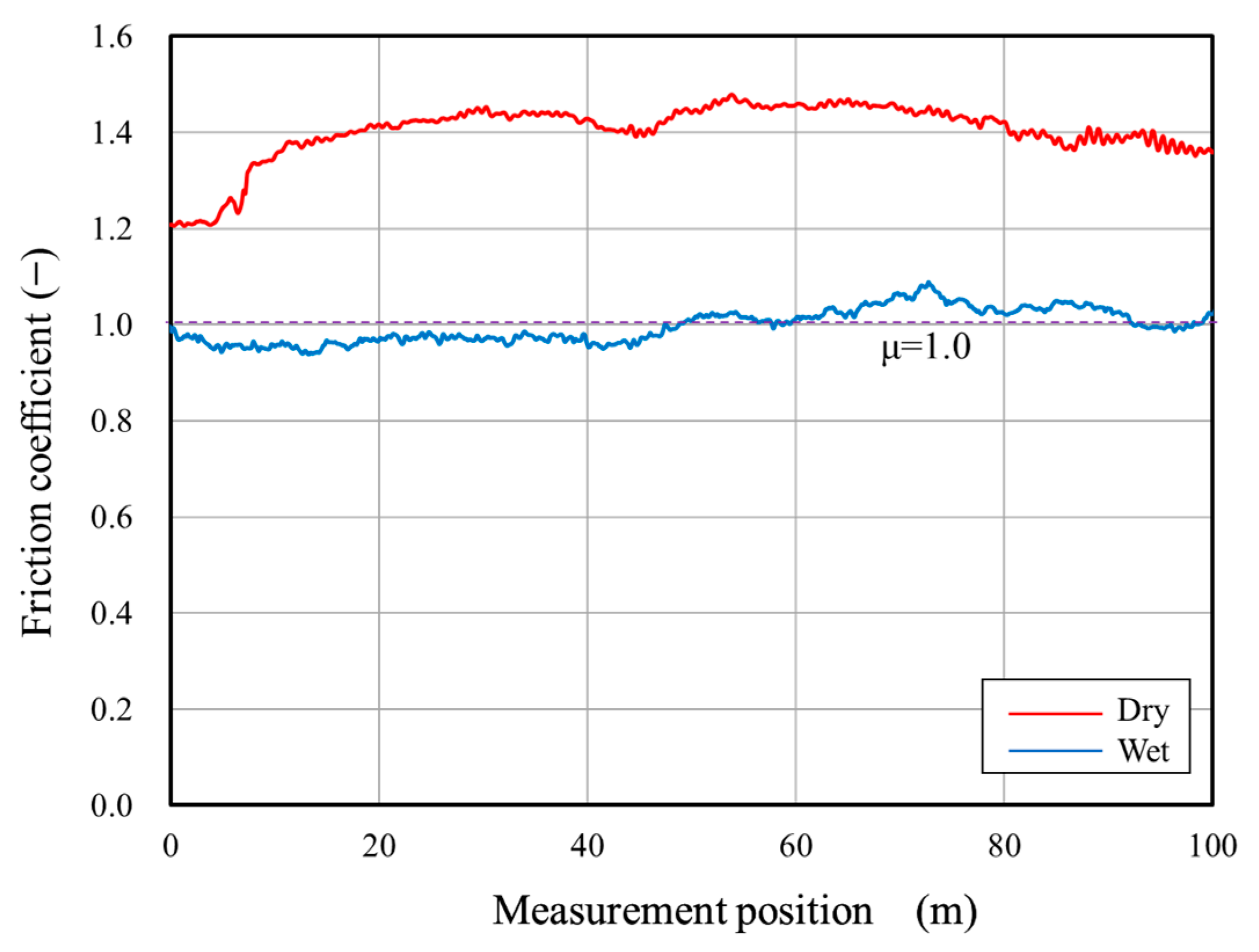
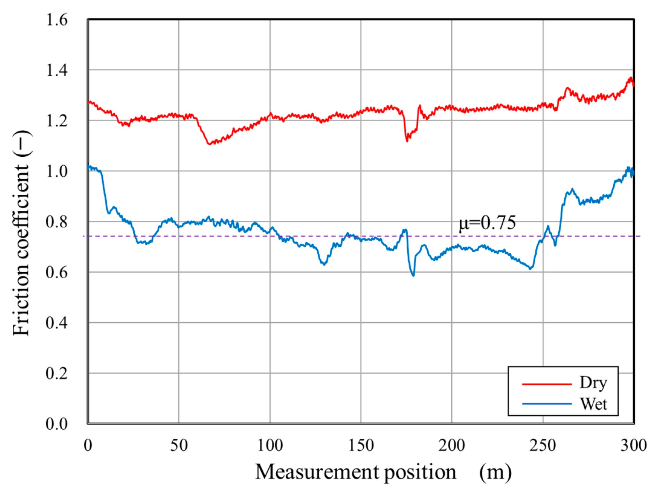
The difference between dry and wet conditions on the road surface was measured at the same position on the road surface. As a result, it was shown that the reduction in the peak μ owing to wet conditions greatly differs depending on the pavement condition. This type of information is essential for improving road traffic safety and developing appropriate measures to mitigate the risks associated with changes in road surface conditions.

(4)

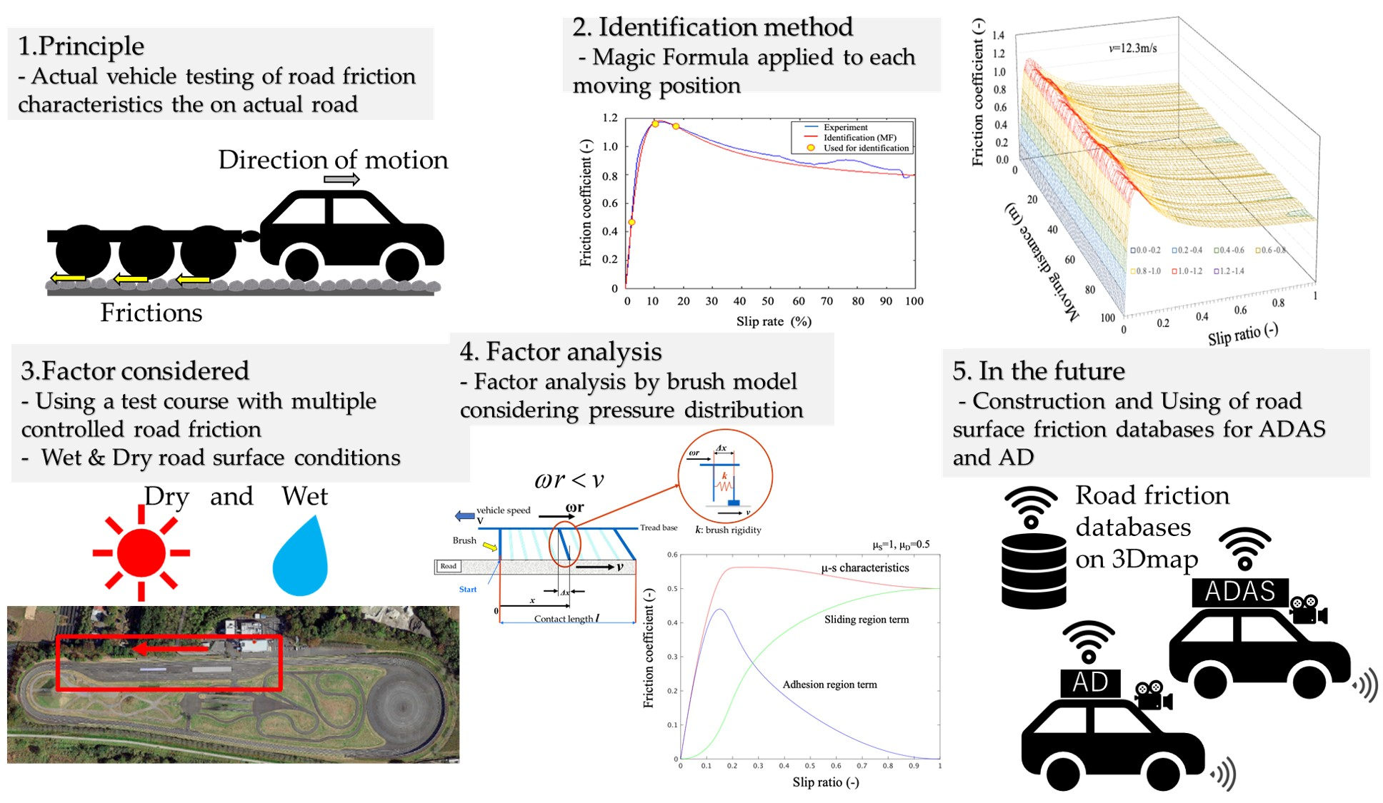
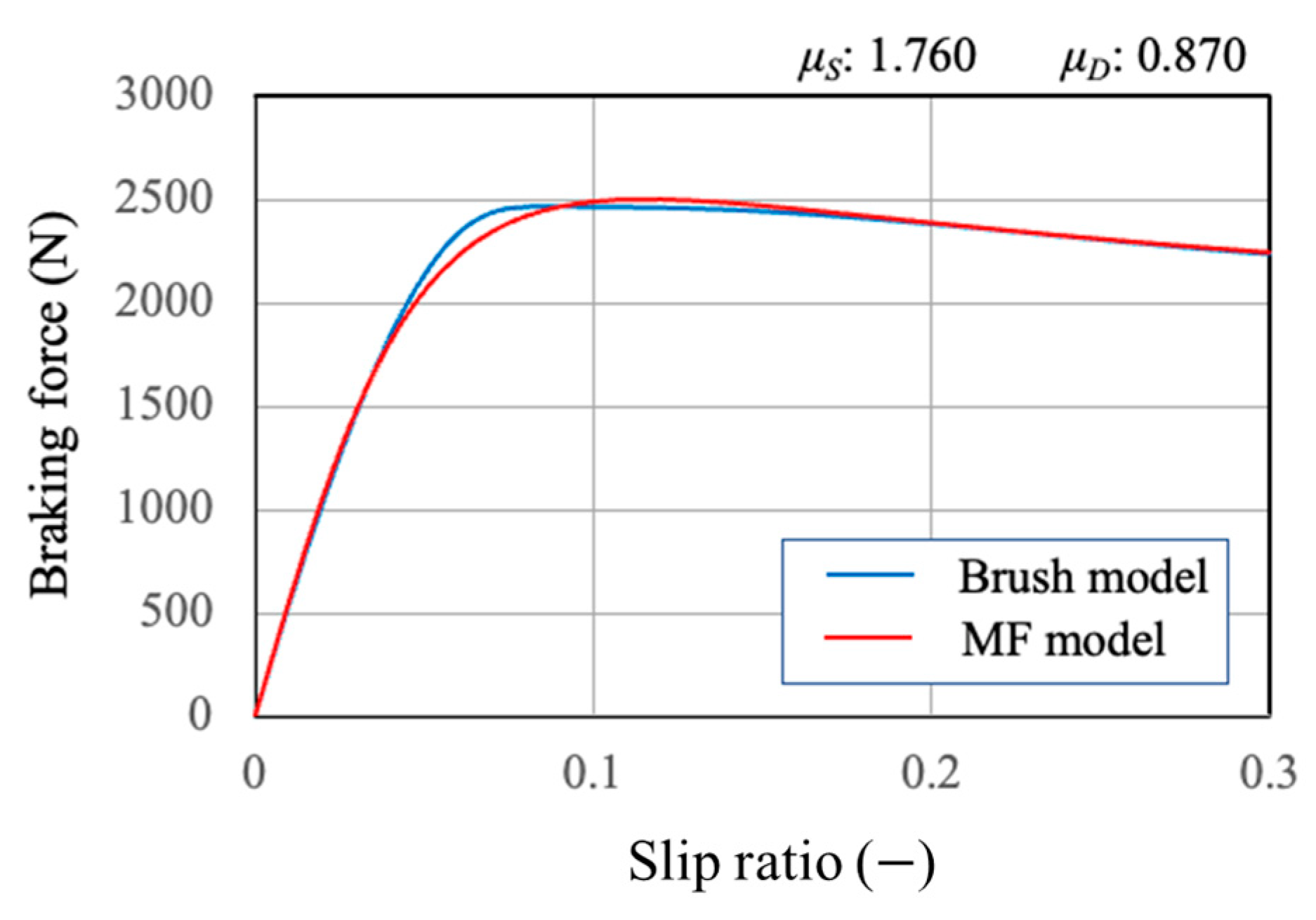
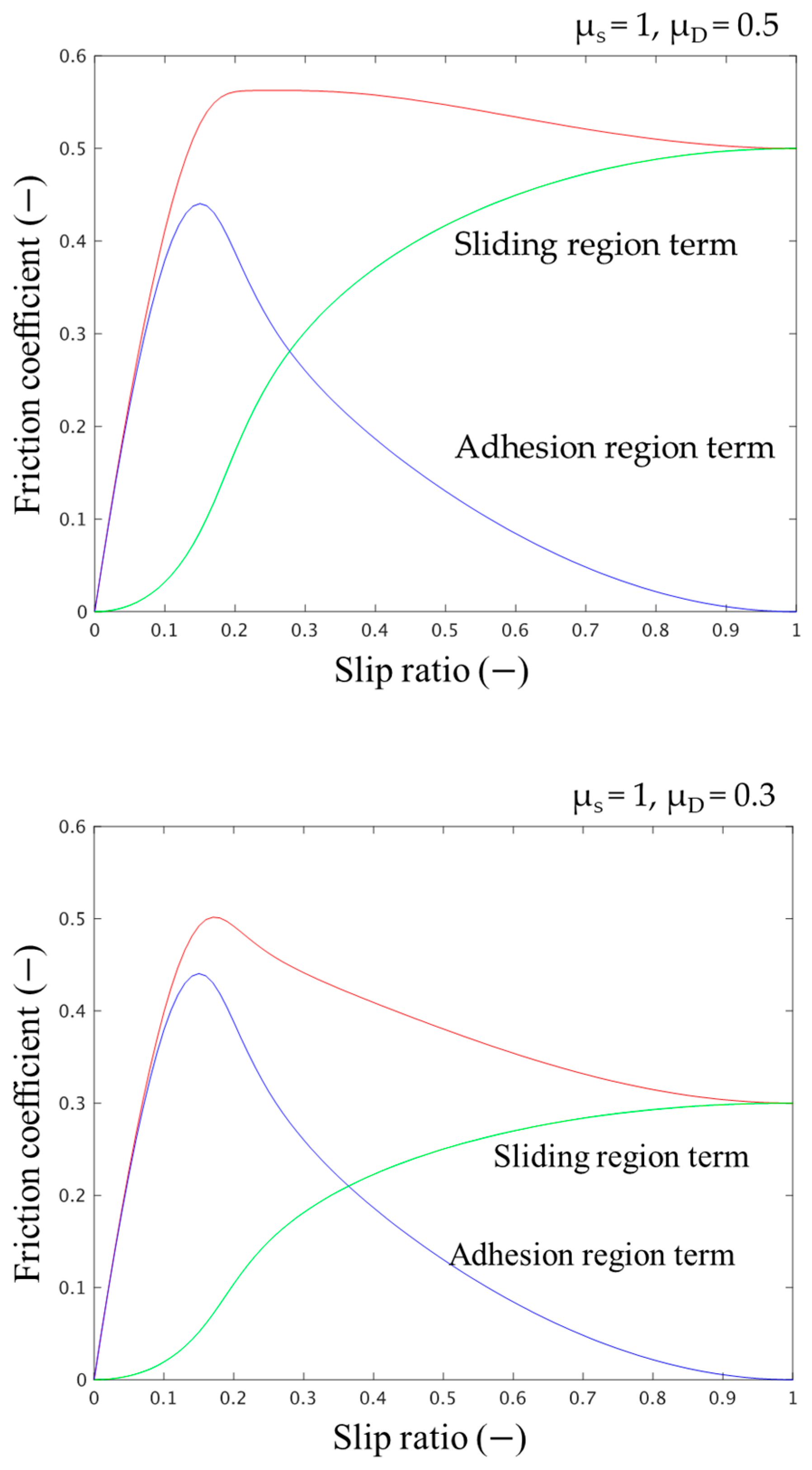
Based on the results of the braking characteristics identified using the MF, the contact surface pressure was used to express the brush model quantitatively, and the maximum static friction and DF of the actual road surface were estimated. Based on this result, the brush model was used to present the adhesion and sliding region components of the μ–s characteristics, and it was shown to have a significant influence on the μ–s characteristic shape.

(5)

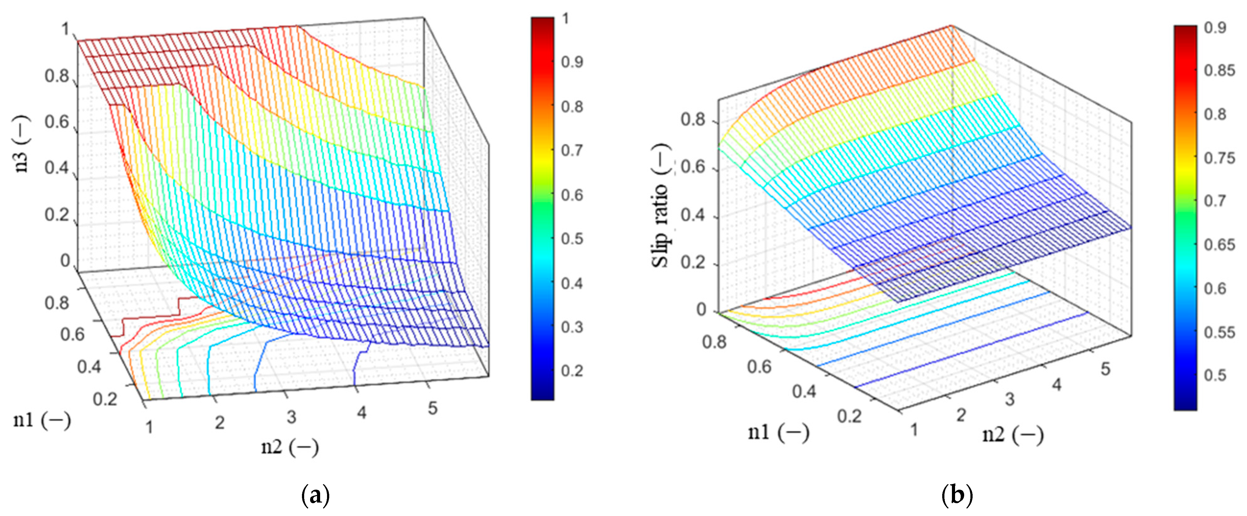
We standardized ${\mu }_D$ and the increasing slope using ${\mu }_s$ and showed that they have a significant influence on the peak μ and slip ratios. Consequently, the possibility of estimating the shape of the μ–s characteristics is demonstrated.

Using this system, road friction measurements were conducted on relatively stable road surfaces, such as a proving ground. Therefore, the effectiveness of this system on uneven, snowy, and frozen road surfaces remains unknown and requires further investigation. In the future, it will be necessary to examine the possibility of estimating the μ–s characteristics by measuring the ${\mu }_s$ and the ${\mu }_D$. By measuring ${\mu }_s$ and ${\mu }_D$, as shown in Figure 20, we can determine the ratio of the adhesion region to the slip region in the μ–s characteristics. This knowledge can be applied, for example, to optimize brake systems. The adhesion region has a high frictional force, resulting in enhanced braking performance. However, the slip region has a lower frictional force, thereby introducing slip and lock risks, which require appropriate control measures.

References

- Pisano, P.A.; Goodwin, L.C.; Rossetti, M.A. US highway crashes in adverse road weather conditions. In Proceedings of the 24th Conference on International Interactive Information and Processing Systems for Meteorology, Oceanography and Hydrology, New Orleans, LA, USA, 20 January 2008. [Google Scholar]
- Andrey, J.; Yagar, S. A temporal analysis of rain-related crash risk. Accid. Anal. Prev. 1993, 25, 465–472. [Google Scholar] [CrossRef] [PubMed]
- Motomatsu, S.; Yamamoto, M. Characteristics of high-performance pavement and pavement diagnosis technology. J. INCE/J 2001, 25, 122–128. (In Japanese) [Google Scholar] [CrossRef]
- Mataei, B.; Zakeri, H.; Zahedi, M.; Nejad, F.M. Pavement Friction and Skid Resistance Measurement Methods: A Literature Review. Open J. Civ. Eng. 2016, 6, 537–565. [Google Scholar] [CrossRef]
- Brown, E.R.; Hainin, M.; Cooley, A.; Hurley, G. Relationship of Air Voids, Lift Thickness, and Permeability in Hot Mix Asphalt Pavements; National Academies of Sciences, Engineering, and Medicine; The National Academies Press: Washington, DC, USA, 2004. [Google Scholar]
- Yan, B. Experimental Study on Wet Skid Resistance of Asphalt Pavements in Icy Conditions. Materials 2019, 12, 1201. [Google Scholar] [CrossRef] [PubMed]
- Christina, P. Quantification of skid resistance seasonal variation in asphalt pavements. J. Traffic Transp. Eng. 2020, 7, 237–248. [Google Scholar]
- Khalfghian, S.; Emami, A.; Taheri, S. A Technical Survey on tire-road friction estimation. Friction 2017, 5, 123–146. [Google Scholar] [CrossRef]
- Watanabe, K.; Kageyama, I.; Kuriyagawa, Y. A Study on Construction of Estimation Algorithm for Road Conditions; The Japan Socity of Mechanical Engineers: Tokyo, Japan, 2002; TRANSLOG 11th, No. 02-50; pp. 71–74. (In Japanese) [Google Scholar]
- Watanabe, K.; Kageyama, I.; Kuriyagawa, Y. Study on Construction of Estimation Algorithm for Coefficient of Road Friction; The Japan Socity of Mechanical Engineers: Tokyo, Japan, 2003; TRANSLOG 12th, No. 03-51; pp. 45–48. (In Japanese) [Google Scholar]
- Alonso, J.; Lopez, J.M.; Pavon, I.; Recuero, M.; Asensio, C.; Arcas, G.; Bravo, A. On-board wet road surface identification using tire/road noise and Support Vector Machines. Appl. Acoust. 2014, 76, 407–415. [Google Scholar] [CrossRef]
- Ise, T. Study on Tactile Sensors for Tires that Can Measure the Friction State of the Driving Surface. Ph.D. Thesis, Kanazawa University, Ishikawa, Japan, 2015. (In Japanese). [Google Scholar]
- Morinaga, H.; Wakao, Y.; Hanatsuka, Y.; Kobayakawa, A. The Possibility of Intelligent Tire (Technology of Contact Area Information Sensing); FISITA2006, Transactions; JSAE: Tokyo, Japan, 2006; Volume F2006V104, pp. 1–11. [Google Scholar]
- Morinaga, H.; Hanatsuka, Y.; Wakao, Y. Sensing Technology Tire System for Road Surface Condition Judgment. FISITA2010 Trans. 2010, F2010E010, 1–8. Available online: https://cir.nii.ac.jp/crid/1572543025664202752 (accessed on 11 May 2023).
- Tuononen, A.J. Optical position detection to measure trye carcass. Veh. Syst. Dyn. 2008, 46, 471–481. [Google Scholar] [CrossRef]
- Bakker, E.; Nyborg, L.; Pacejka, H.B. Tyre Modelling for Use in Vehicle Dynamics Studies; SAE Paper No. 870421; SAE International: Warrendale, PA, USA, 1987. [Google Scholar]
- Tielking, J.T.; Fancher, P.S.; Wild, R.E. Mechanical Properties of Truck Tires; SAE Paper No.730183; SAE International: Warrendale, PA, USA, 1973. [Google Scholar]
- Tezuka, Y.; Ishii, H.; Kiyota, S. Application of the Magic Formula Tire Model to Motorcycle Maneuverability Analysis. JSAE Rev. 2001, 22, 305–310. [Google Scholar] [CrossRef]
- Pacejka, H.B.; Bakker, E. The Magic Formula Tire Model. Int. J. Veh. Mech. Mobil. 1992, 21, 1–18. [Google Scholar]
- Pacejka, H.B.; Besselink, I.J.M. Magic Formula Tire Model with Transient Properties. Int. J. Veh. Mech. Mobil. 1997, 27, 234–249. [Google Scholar]
- Pacejka, H.B. Tire and Vehicle Dynamics; Butterworth-Heinemann: Oxford, UK, 2005. [Google Scholar]
- Fiala, E. Seitenkraefte am rollenden Luftreifen (Lateral forces acting on pneumatic tire). Ver. Dtsch. Ing. –VDI Z. 1954, 96, 973–979. [Google Scholar]
- Svendenius, J.; Wittenmark, B. Brush tire model with increased flexibility. In Proceedings of the 2003 European Control Conference (ECC), Cambridge, UK, 1–4 September 2003. [Google Scholar]
- Jacob, S. Wheel Model Review and Friction Estimation, Technical Report TFRT—7607–SE; Department of Automatic Control, LTH Studiecentrum: Lund, Sweden, 2003. [Google Scholar]
- O’Neill, A. Enhancing brush tire model accuracy through friction measurements. Int. J. Veh. Mech. Mobil. 2022, 60, 2075–2097. [Google Scholar]
- Lu, Q.; Steven, B. Friction Testing of Pavement Preservation Treatments: Literature Review. UCPRC-TM-2006-10. Compare. 1971. Available online: https://escholarship.org/uc/item/3jn462tc (accessed on 11 May 2023).
- Liew, T.H. New Apparatus for Skid Testing: Assessment for Dusty Surfaces (Malaysia: Universiti Teknologi Malaysia). 2002. Available online: eprints.utm.my/id/eprint/5808/1/71937.pdf (accessed on 11 May 2023).
- Abe, Y. Development and Use of Portable Slip Resistance Measuring Devices for Road Surfaces. Ph.D. Thesis, Muroran Institute of Technology, Hokkaido, Japan, 2000. (In Japanese). [Google Scholar]
- Zaid, N.B.M.; Hainin, M.R.; Idham, M.K.; Warid, M.N.M.; Naqibah, S.N. Evaluation of Skid Resistance Performance Using British Pendulum and Grip Tester. IOP Conf. Ser. Earth Environ. Sci. 2019, 220, 012016. [Google Scholar] [CrossRef]
- Kageyama, I.; Kuriyagawa, Y.; Haraguchi, T.; Kaneko, T.; Asai, M.; Matsumoto, G. Study on the Road Friction Database for Automated Driving: Fundamental Consideration of the Measuring Device for the Road Friction Database. Appl. Sci. 2021, 12, 18. [Google Scholar] [CrossRef]
- Kageyama, I.; Kuriyagawa, Y.; Haraguchi, T.; Kaneko, T.; Nishio, M.; Watanabe, A. Study on Road Friction Database for Traffic Safety: Construction of a Road Friction-Measuring Device. Inventions 2022, 7, 90. [Google Scholar] [CrossRef]
- Kageyama, I.; Kuriyagawa, Y.; Haraguchi, T.; Kaneko, T.; Nishio, M.; Watanabe, A.; Matsumoto, G. Study on Evaluation of Road Friction Characteristics on Ordinary Roads. Trans. Soc. Automot. Eng. Jpn. 2023, 54, 594–601. (In Japanese). Available online: https://cir.nii.ac.jp/crid/1390014735381153792 (accessed on 11 May 2023).
- Kageyama, I.; Kuriyagawa, Y.; Haraguchi, T.; Kaneko, T.; Asai, M.; Tahira, S.; Matsumoto, G. Study on Measurement of Road Friction Characteristics and Estimation Method for Tire Characteristics—Relationship between Longitudinal and Lateral Forces. Trans. Soc. Automot. Eng. Jpn. 2022, 53, 213–218. (In Japanese). Available online: https://www.safetylit.org/citations/index.php?fuseaction=citations.viewdetails&citationIds[]=citjournalarticle_742701_29 (accessed on 11 May 2023).
- Sakai, H. Tire Engineering; Guranpuri-Shuppan: Tokyo, Japan, 1987; p. 120. (In Japanese) [Google Scholar]