Article

Performance Prediction Model for Hydrodynamically Lubricated Tilting Pad Thrust Bearings Operating under Incomplete Oil Film with the Combination of Numerical and Machine-Learning Techniques

by
Konstantinos P. Katsaros
* and
Pantelis G. Nikolakopoulos
Machine Design Laboratory, Department of Mechanical Engineering and Aeronautics, University of Patras, 26504 Patras, Greece
*
Author to whom correspondence should be addressed.
Lubricants 2023, 11(3), 113; https://doi.org/10.3390/lubricants11030113
Submission received: 23 January 2023 / Revised: 25 February 2023 / Accepted: 1 March 2023 / Published: 4 March 2023
(This article belongs to the Special Issue Recent Advances in Machine Learning in Tribology)

Abstract

:
Pivoted pad thrust bearings are common machine elements used in rotating mechanisms in order to support axial loads. The hydrodynamic lubrication of such bearings has been a major subject of many investigations over the years. However, the majority of these investigations are based on full film lubrication models, when, in fact, incomplete oil film profiles appear during various operating conditions, such as startups and shutdowns. The lack of lubricant during operations can have severe impact on the bearing’s performance, affecting its ability to carry the applied axial load. The scope of the current investigation is to combine numerical analysis and machine-learning techniques in order to create a model that predicts the thrust bearing’s performance in terms of the pad’s load-carrying capacity. For this purpose, the 2-D Reynolds equation is solved numerically for a variety of angular velocities and three different lubricants: SAE 20, SAE 30 and SAE 10W40. The position of the lack of lubricant within the oil film’s control volume is studied and evaluated, together with the percentage of oil film coverage in the inlet of the pad. The results of the numerical analysis are used as input, in order to train and evaluate three different machine-learning models: Quadratic Polynomial Regression, Quadratic SVM Regression and Regression Trees. The results showed that the position of the film incompleteness affects the ability of the bearing to carry the axial load. At the same time as less lubricant entered the domain, the pressure drop could reach lower values, up to 93%. From the studied lubricants, SAE 10W40 was the one that showed the best performance results during incomplete oil film operation. Finally, the Quadratic Polynomial Regression model showed the best fit and 99% accuracy in predicting the pad’s load-carrying capacity.

1. Introduction

Over the years, hydrodynamically lubricated tilting pad thrust bearings have been widely used in many applications, such as agriculture, electrical generators, mining, naval and automotive industry. They are designed to carry axial loads of rotating machinery based on the hydrodynamic principals. A wedge created from the stationary thrust pads and the rotor, as well as the relative motion of these two friction surfaces with the lubrication film flowing in the middle, describe the fundamental principal of operation for such bearings. Many researchers have built computational algorithms in order to model the flow of the lubricant inside these mechanisms and calculate the major tribological parameters that affect the operation of the bearings [1,2,3,4]. At the same time, a wide variety of lubricants, surface profiles, texturing and coatings have been investigated in order to improve pad thrust bearings’ operation targeting to maximize the load-carrying capacity with the minimum possible power losses [5,6,7,8]. The majority of these studies are based on the assumption of a full lubricant film along the pad’s surface. However, in many applications, the lubricant’s flow in the inlet of the pad is not sufficient enough to cover the full width, resulting in incomplete oil film operating conditions. Such operating conditions can occur in several occasions, such as in startups and shutdowns, as well as in cases of direct lubrication, regardless of the supply method. This oil film incompleteness can result in severe pressure drop inside the pad, reducing the bearing’s load-carrying capacity. To begin with, Etsion et al. [9] used the finite difference technique to solve the Reynolds equation for a flat, sector-shaped pad thrust bearing with incomplete oil film. By calculating and comparing the bearing’s load-carrying capacity and power loss with the results of a complete fluid film bearing, they concluded that the bearing’s performance was affected by the location of the lubricant’s supply. Furthermore, Heshmat et al. [10] performed a parametric study on thrust bearings with insufficient oil supply. They investigated different numbers of pads and inner and outer radii, as well as multiple degrees of starvation for tapered land bearings. The results showed that 12-pad thrust bearings with (R2 − R1)/R2 = ½ were the optimum geometry under starved conditions. Finally, Artiles and Heshmat [11] performed an analysis on starved thrust bearings that included temperature effects. They used a finite difference mesh in order to solve the 2-D temperature and pressure fields. The investigation was performed for tapered land thrust bearings for different minimum film thicknesses and levels of starvation. It was found that the effects of starvation were small when the bearing was flooded with lubricant, but accelerated rapidly below 50% of starvation level. The start of the film was mainly independent of geometric characteristics, but directly dependent on the starvation level.
Modern technological advances in the field of computer engineering and networks have already positively affected the more traditional mechanical engineering in many aspects. The so-called 4th Industrial Revolution has provided researchers with impressive computational power and digital tools, such as AI, machine-learning and IoT: enough to support more revolutionary investigations and applications. In the field of tribology, and specifically in bearings, researchers have mainly applied these tools for fault diagnosis, prognosis and residual life estimation. It was not until recently that progress was reported in applying such techniques on the design and performance prediction of bearings. First of all, A. Moosavian et al. [12] proposed a diagnostic method that can reliably separate different fault conditions for the main journal bearings of an internal combustion engine. Vibration signals of three different operating conditions were examined (normal, oil starvation and extreme wear) and then used as inputs to train two classifiers: K-nearest neighbor and artificial neural network. The artificial neural network showed better performance in journal bearing fault diagnosis compared to the K-nearest neighbor classifier. Furthermore, Alves et al. [13] presented promising results for training machine-learning algorithms with simulated data in order to perform ovalization fault diagnosis in hydrodynamic journal bearings. They built a numerical model to simulate the ovalization fault conditions; then, they used the numerical analysis results as a training data set for a deep convolutional neural network algorithm that was able to predict the fault conditions. Moreover, S. Poddar and N. Tandon [14] developed an application that takes acoustic emission data as input and diagnoses the category of faults in journal bearing operation. To do so, they used acoustic emission signals from journal bearings operating under normal conditions, cavitation, particle contamination and oil starvation. These data were then used in order to train different decision tree and K-nearest neighbor machine-learning models. The weighted k-NN classifier model showed the best prediction results and was eventually used for the application. R.L. Lorza et al. [15] proposed a combined Finite Element and Data Mining method to determine the maximum load-carrying capacity in tapered roller bearings. The FE model was run for different input loads and the corresponding contact stresses were obtained. This training data set was then used to train a regression model. Linear regression, Gaussian processes, artificial neural networks, support vector machines and regression trees were investigated in this study. The best combination of input loads was achieved by applying evolutionary optimization techniques based on genetic algorithms to the best regression models. In addition, K.P. Katsaros and P.G. Nikolakopoulos [16] proposed a combination of numerical and machine-learning techniques in order to identify optimal designs in hydrodynamically lubricated pivoted pad thrust bearings. A 2-D Reynolds-based finite difference numerical model was solved for three different lubricants and multiple operating conditions. The obtained tribological data were then used to train linear, quadratic and SVM regression models. AWS 100 was found to be the most efficient lubricant; it showed the maximum load-carrying capacity and the minimum friction force for the thrust pad. Moschopoulos et al. [17] developed a machine-learning procedure in order to predict journal bearings’ performance characteristics. To this end, they recorded sound and vibration signals, applying the one-third octave filter to post process them. With this data set, they trained three ML algorithms: K-nearest neighbor, random forest classifier and gradient-boosting regressor. The investigation showed that ML algorithms that used sound signals had better prediction accuracy compared to those based on vibration signals. Finally, Zavos et al. [18] proposed a machine-learning approach, in order to design piston rings and thrust bearings with optimum coating selection. For this purpose, analytical results from the friction models of both assemblies were used as input data in order to train quadratic polynomial regression and support vector machine models. By predicting the minimum friction coefficient, the investigation showed that, in the case of piston rings, the TiN2 and TiAlN were the best design selection. On the other hand, in the case of the tiling pad thrust bearing, the DLC was the optimum coating selection.
The aim of this study is to combine numerical and machine-learning algorithms in order to create a model that predicts the performance of tilting pad thrust bearings that operate under various incomplete oil film profiles. Focusing on the load-carrying capacity of the pad as a critical performance characteristic, the pad bearing’s operation is simulated for rotational velocities from 2000 up to 12,000 rpm. Three lubricants are used during the investigation: the mono-grade oils SAE 20 and SAE 30, as well as the multi-grade SAE10W40. Three different machine-learning methods (quadratic polynomial regression, support vector machine, regression trees) are applied and compared in terms of predictions accuracy. The novelty of this study lies in the fact that no similar work can be found in literature combining numerical and ML methods for incomplete oil film study and design of hydrodynamically lubricated tilting pad thrust bearings.

2. Theory

2.1. Hydrodynamic Lubrication Model

The 2-D Reynolds Equation (1) is used in the current study in order to calculate the hydrodynamic characteristics of the lubricant’s flow. The pivoted pad under consideration is approximated and considered to be a center-pivoted rectangle. A schematic of the rotor–pad conjunction is presented in Figure 1. The film thickness is assumed to be small compared to the length and the width of the pad. To add to that, Newtonian, incompressible lubricants are assumed to follow a laminar and isothermal flow inside the pad- rotor conjunction. Cavitation effects, although important in specific pad geometries and high rotational velocities, are not taken into consideration for the current investigation, based on the assumption that the minimum pressure is not reaching the vapor pressure value. In the rotor-lubricant interface, the oil is assumed to gain the velocity of the wall that it comes in contact with; thus, the no-slip condition is applied [19]. Moreover, the viscosity is considered to be constant throughout the film thickness. The film thickness h is assumed to be a function of the pad’s length and is calculated from equation (2), while any change in the radial direction and the corresponding misalignment issues are not taken into consideration. Normally, the inclination of the pad and the minimum film thickness are calculated at the equilibrium position, so that the pad can carry the applied load. In this study, given the specific minimum film thickness and the inclination value, the load-carrying capacity of the pad is calculated in the equilibrium position by integrating the pressure p over the bearing pad area (3). In the cases of incomplete oil film, the lubricant’s width (l) is calculated based on the continuity of the flow (4).
x ( h 3 p x ) + y ( h 3 p y ) = 6 μ U h x
h = f ( x ) = h 1 + x B ( h 1 h 0 )
F p = A p d A = W
0 l q x d y = 0 L 0 ( q x ) 0 d y ± 0 L q y d x

2.2. Viscosity Model

During operation, the rise in temperature leads to a decrease in the lubricant’s viscosity value. As mentioned, from Nacer Tala-Ighil and Michel Fillon [20], the concept of the “effective temperature” can be considered in order to approximate the operating viscosity value without applying complex and time-consuming THD algorithms. The effective temperature value inside the lubricant’s domain is calculated from Equations (5) and (6) [21]. T is the effective temperature of the lubricant, while T0 is considered to be the inlet temperature. The constant ke is empirical and, with a value of 0.8, gives good agreement between theory and experiment. The variation of temperature ΔT is considered to be a function of friction, rotating velocity and average axial fluid flow. The lubricant’s density and specific heat capacity are also taken into consideration. To add to that, the fraction l i n L is applied, in order to define the various percentages of inlet oil coverage during the investigation. An iterative procedure is followed, in order to define the final average effective temperature for each simulation.
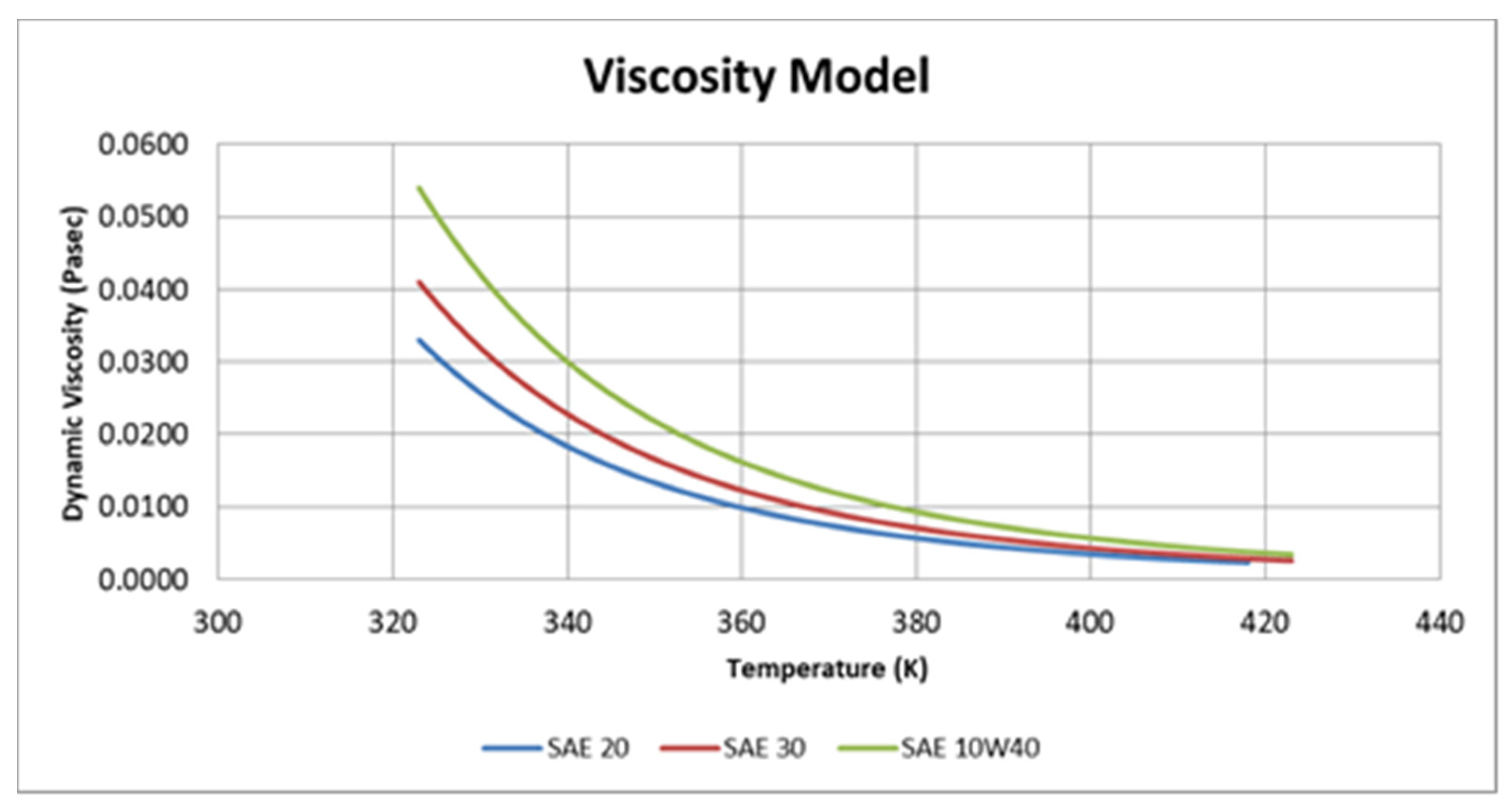
The Sutherland’s law is used to model the viscosity variation according to temperature (7), (8). Specific coefficients are calculated as the model is adapted to fit the known dynamic viscosity values for each lubricant. A graphical representation of the dynamic viscosity variation according to temperature is shown in Figure 2.
T = T 0 + k e Δ T
Δ T = 2 F U l i n L Q ρ σ
μ = μ ν e A
A = C 2 μ ( 1 Τ + 1 C 1 μ ) + C 3 μ ( 1 Τ + 1 C 1 μ )

2.3. Numerical Analysis

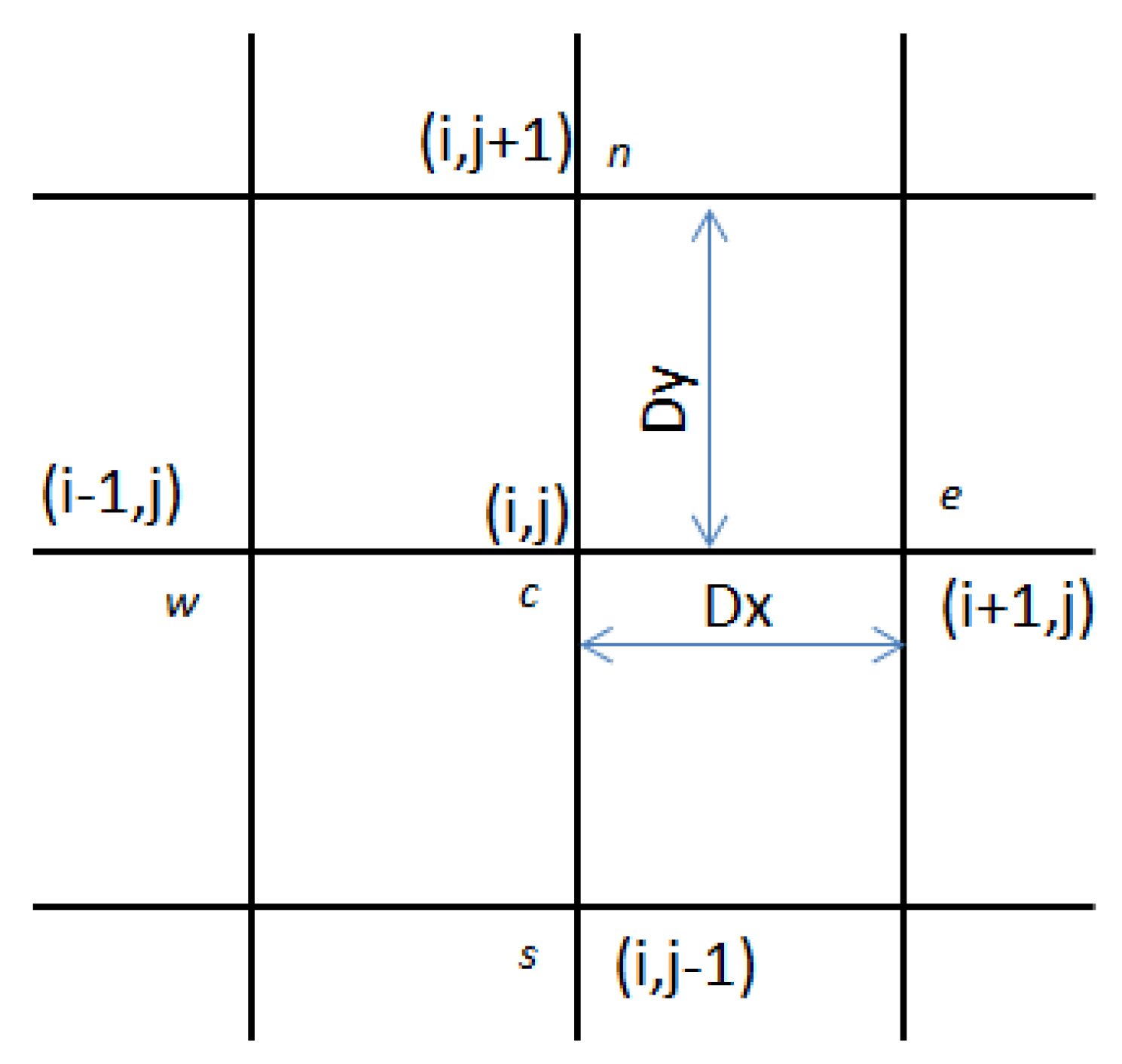
In order to numerically solve the Reynolds equation, the control domain of the lubricant inside the pad-rotor tribocouple is discretized with a typical 2-D mesh of approximately 2500 finite cells; 50 in x direction, and 50 in y direction. Spatial resolution tests showed differences in the order of 1% between typical and fine meshes. The inlet and outlet of the lubricant’s control volume are assumed to be openings, and a constant pressure P = patm is applied as a boundary condition. To add to that, an outflow condition is prescribed in both inner and outer pad sides: r = Rin, Rout. In addition, no inflow is allowed in the computational domain and the ambient pressure P = patm is applied. The rotor is assumed to be moving with a constant rotational velocity ω, which corresponds to U = ωrmean at the pad’s mid sector. An iterative algorithm is built based on the finite differences—central differences—methodology. The Reynolds equation is adapted so that the algorithm is able to swipe over the grid and compute the corresponding pressure Pij at any internal node (9). A representation of the calculation is presented in Figure 3, where c is the node at which the pressure is calculated and n, w, s, e are the neighboring nodes used for this calculation. Convergence to steady-state condition is verified by monitoring the computed nodal pressure based on the defined convergence criteria (10). In the cases of incomplete oil film (Figure 4), the lubricant’s width limit lines LB (i), LT (i) are calculated by swiping over the nodes in the direction of the flow (11). The amount of lubricant that enters the domain lin flows through the pad-rotor conjunction and adapts to the inclination of the pad. As a result, the same amount of lubricant at every step of the way through the pad (i) has to cover more and more of its surface until (if) it reaches the pad’s sides or the end of the pad in the flow direction. Pressure P = patm is then applied as a boundary condition on the area where no lubricant flows. The calculation of pressure distribution in the y-direction is then limited to the new boundary conditions. In addition, Case A refers to lack of lubricant on the outer part of the pad, and is modeled with LB (i) placed on the inner pad border, while LT (i) takes values within the domain. Case B refers to the lack of lubricant on the inner part of the pad. As a result, LT (i) is placed on the outer border and LB (i) runs through the fluid film domain. Finally, Case C refers to the scenario where both LB (i) and LT (i) are calculated symmetrically through the fluid film.
P i , j = C n P n + C w P w + C s P s + C e P e + G       i , j = 0 , , 50
E r r p r e s s = 1 N | P i j P i 1 j | 1 N | P i j | 1 × 10 6
l i = l i n h i n h i
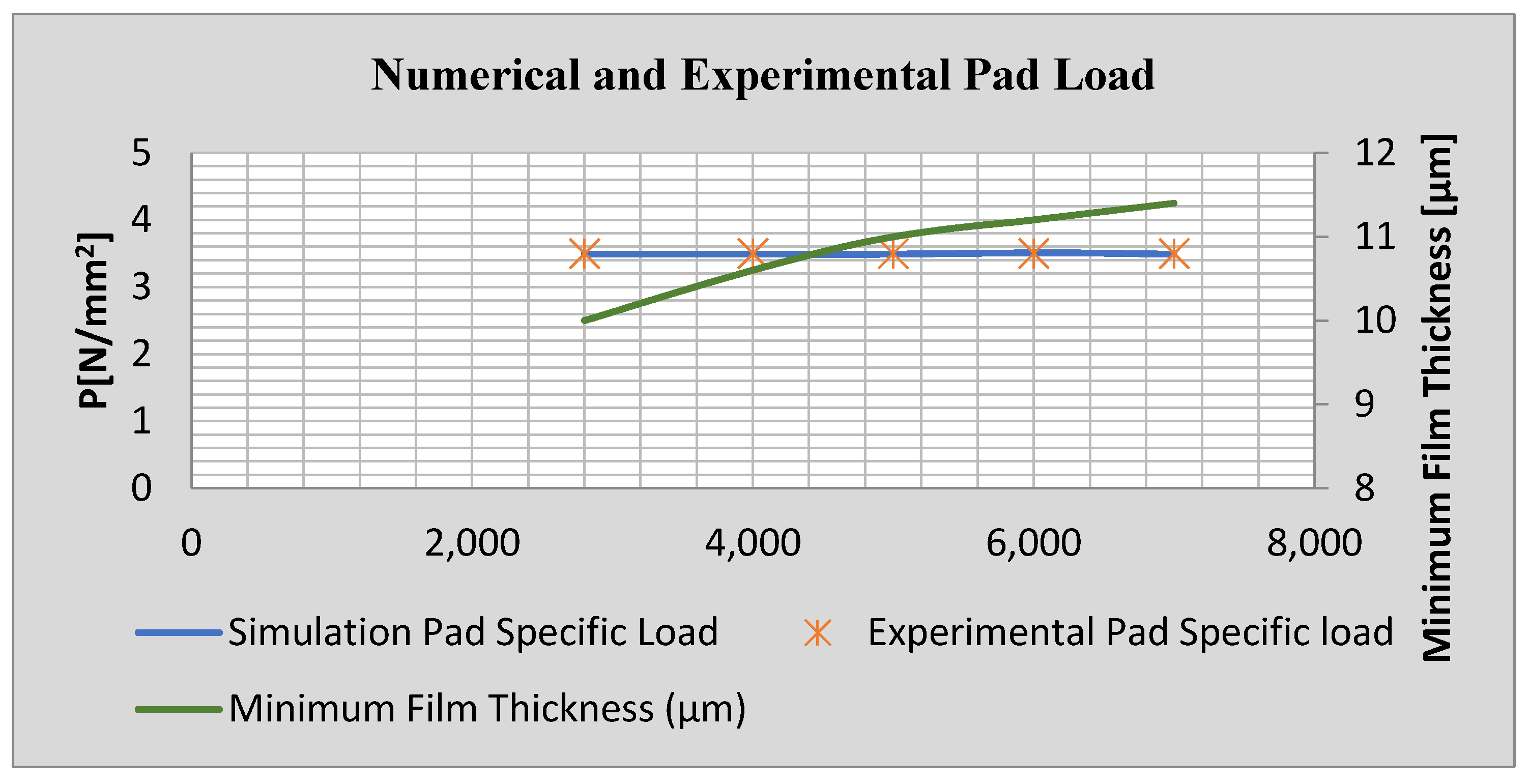
The hydrodynamic lubrication model is validated with experimental data obtained from the paper of Bielec and Leopard [22]. Figure 5 shows that there is a good agreement between the experimental and computed pad-specific load for different angular velocities and film thicknesses.

2.4. Machine-Learning

For the purpose of this study, all the data obtained from the numerical simulations are used as input, in order to train and compare machine-learning models based on three different methods: the Multi-Variable Quadratic Polynomial Regression, the Quadratic Support Vector Machine and Regression Trees. These regression models are widely used in machine-learning applications, mainly due to their simplicity and accuracy to predict the corresponding response values. To begin with, the Multi-Variable Quadratic Polynomial Regression model is based on the least-squares fit methodology, in which the sum of the squares of the residuals needs to be minimized. Two independent variables, or predictors, are used x1i: rotational velocity [rpm]; x2i: percentage of inlet oil coverage, in order to predict the response values of one dependent variable Y: Pad’s Load-carrying Capacity [N]. For a set of n-observations, Equation (12) or, in matrix form, Equation (13), is solved, in order to calculate the y-intercept: β0 and the corresponding slopes: β1,…,β5.
Y =   XB  
Y = [ y 1 y 2 y n ] = [ 1 x 11 x 21 x 11 2 x 11 x 21 x 21 2 1 x 12 x 22 x 12 2 x 12 x 22 x 22 2 1 x 1 n x 2 n x 1 n 2 x 1 n x 2 n x 2 n 2 ] [ β 0 β 1 β 2 β 3 β 4 β 5 ]  
Furthermore, the Support Vector Machine models were trained in Matlab’s Regression Learner application, using the quadratic polynomial kernel function (14). In addition, with the same application, regression trees were trained and evaluated accordingly. To perform the analysis, all data were sorted in ascending order for both predictors, x1i and x2i. Then, all the mean squared errors were calculated separately for all the response values of both predictors (15) in each splitting candidate node t. At every iteration, the splitting node t of the regression tree was defined as the one that provided the minimum mean-squared error from all the examined data. The procedure continues repeatedly until each branch reaches the pre-defined leaf size. For the current study, a leaf size equal to 4 has been selected, as it provides the finest tree results for the Matlab’s application with the optimum accuracy. In addition, the criteria chosen in the current study, in order to measure and evaluate the goodness of fit for the generated machine-learning models, is the coefficient of determination, or R2 (16). This coefficient indicates the difference between the values of the dependent variable yfit calculated from the model and the observations ynum obtained from the relevant numerical simulations. The higher the value of R2, the better the model is at predicting the data. Finally, the Matlab’s standard 5-fold, cross-validation procedure was applied for 5 randomly chosen partitions of the original data set. All the models where trained with 80% of the data from the data lake, while the rest 20% of the data was used for testing. Experimental data were used for the validation of the ML model as shown in [16].
( X , Y ) = ( c + X T Y ) 2
M S E = 1 n ( y i y t ¯ ) 2
R 2 = 1 1 n ( y num y fit ^ ) 2 1 n ( y num y ¯ ) 2  

3. Results

The simulations were performed for three different types of inlet incomplete oil profiles: Case A: where there was lack of oil on the outer radius; Case B: where there was lack of oil on the inner radius; Case C: symmetrical lack of oil from the center of the pad. Three different lubricants were examined: the mono-grade SAE 20 and SAE 30, as well as the multi-grade SAE 10W40. The simulations were run for rotational velocities, from 2000 up to 12,000 rpm, and a k = 0.1 inclination of the pad. The corresponding Reynolds numbers vary from Re = 60 up to Re = 200, indicating a laminar flow. The coverage of the pad’s inlet with lubricant varied from 1 (full film lubrication) up to 0.4 (40% of the inlet covered with oil). The film thickness variation to rotational velocity has been considered similar to the one presented in Figure 13.3a from Bielec and Leopard [22]. All the input parameters are shown in Table 1.
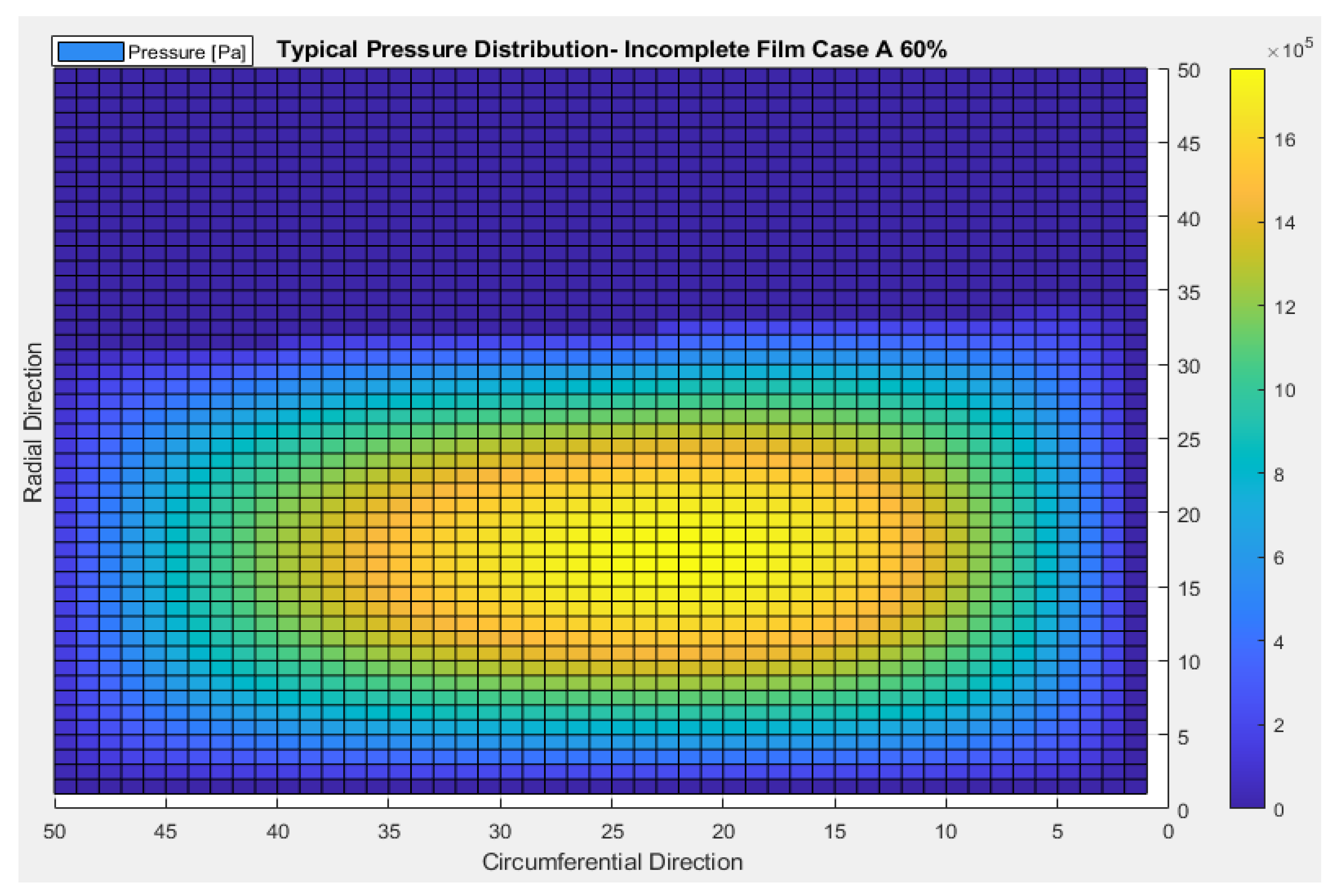
Figure 6, Figure 7 and Figure 8 below show typical representations of the corresponding pressure profiles for the three different incomplete oil film cases studied: A, B, C, at 60% inlet coverage and 6000 rpm rotational velocity.
The total amount of 2079 simulation data was used as input in order to train the machine-learning models that predict the load-carrying capacity of the pad according to rotational velocity and the percentage of oil coverage in the inlet of the pad. Table 2 shows all the Quadratic Polynomial Regression ML models, along with the corresponding R2 values of each case:
The R2 values in all models are close to 0.99, which means that there is a good agreement between the numerical data and the prediction models’ response values. At the same time, this is also an indicator of 99% accuracy for the ML model to predict the pad’s load-carrying capacity at the given predictor values.
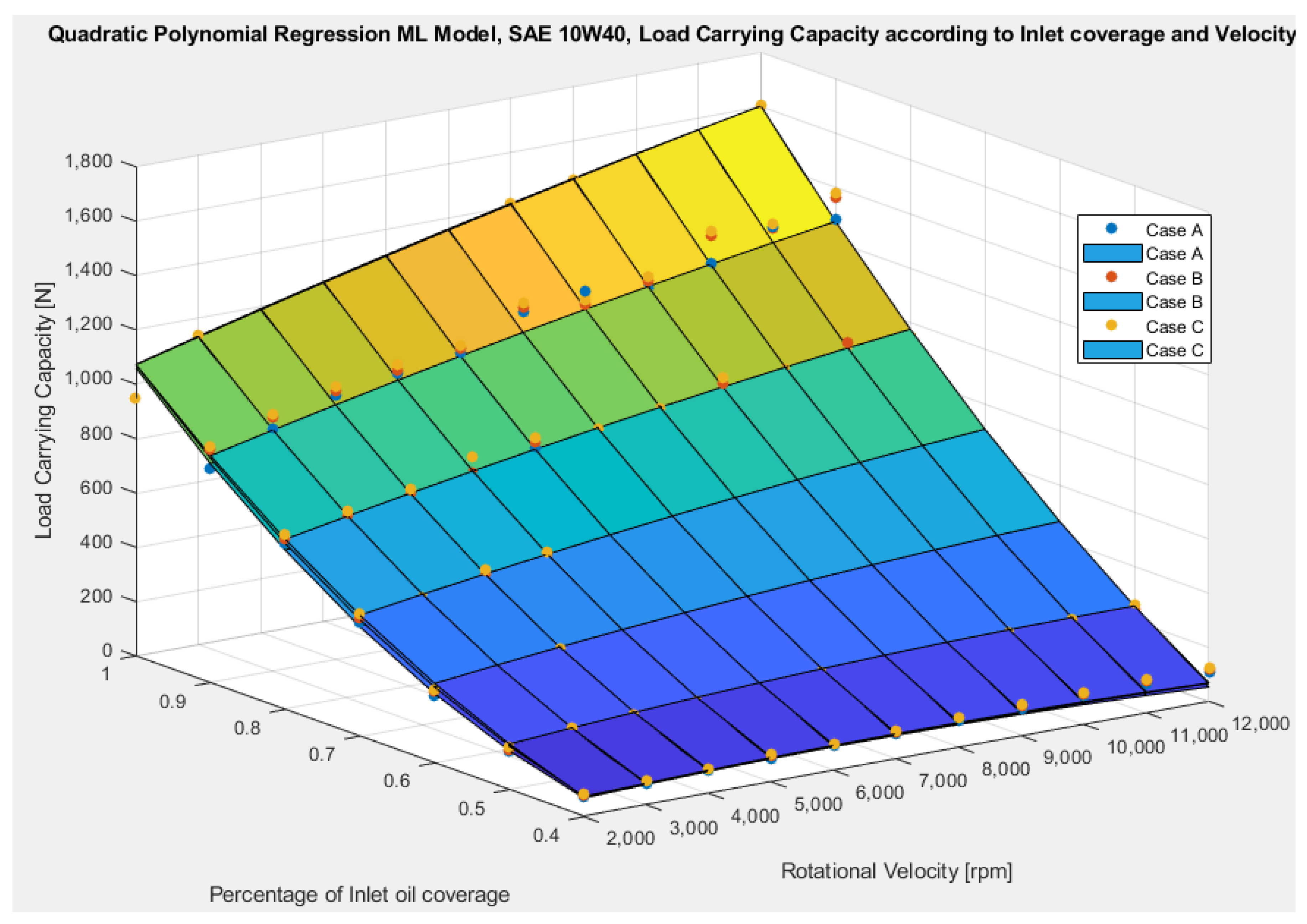
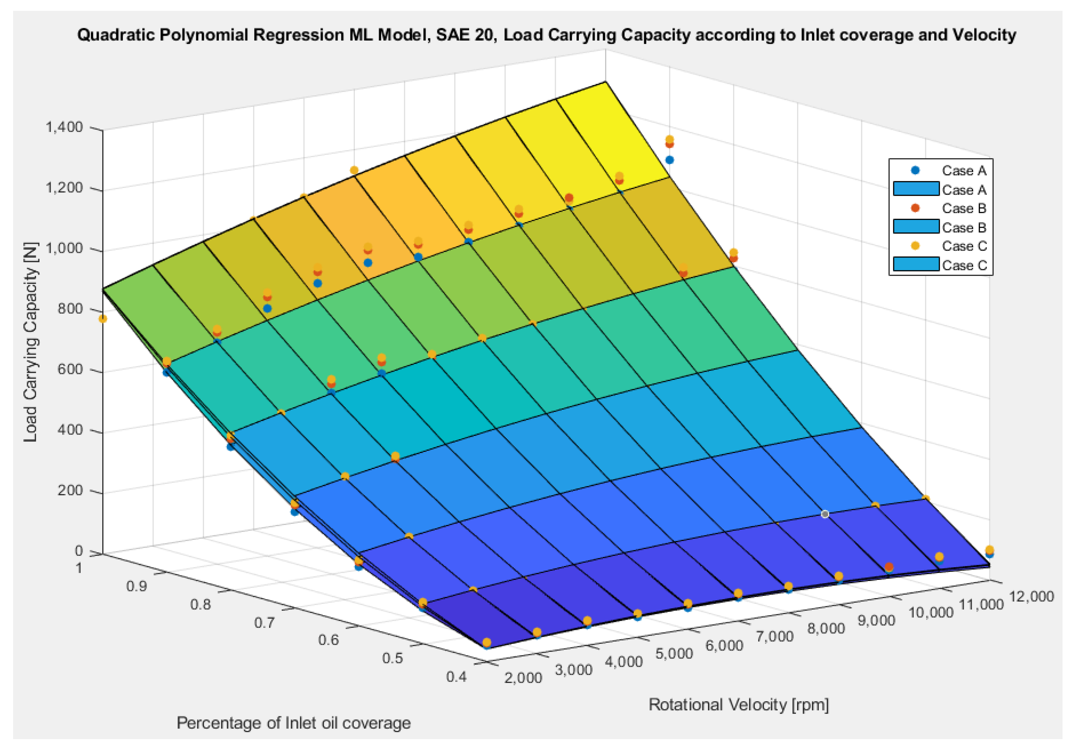
Figure 9, Figure 10 and Figure 11 are the graphical representations of the Quadratic Polynomial Regression ML models for all three lubricants and incomplete oil film profiles. In all cases, the load-carrying capacity of the pad decreases along with the percentage of inlet oil coverage, with the pressure drop reaching up to 93% for 40% inlet oil coverage. Furthermore, it is clearly shown that, in all cases, the lack of lubricant in the outer area of the pad—profile A—shows the minimum load-carrying capacity for the pad. On the other hand, profile C, with the symmetrical lack of lubricant, shows the maximum load-carrying capacity for the pad in all the studied cases. All three lubricants show identical response to the area of oil film incompleteness. Regardless of the angular velocity, data show a better load-carrying capacity for the profile C compared to the profile A, from 6 up to 15%, depending on the coverage of the inlet with oil. As the percentage of the lubricant’s coverage decreases, the case C profile shows better and better performance for the pad of the bearing compared to the profiles A and B. For the worst studied conditions, 12,000 rpm rotational velocity and 40% of inlet oil coverage, the profile C provides up to 15% more load-carrying capacity for the pad compared to the case A profile.
Figure 12 shows the comparison results for Case C—symmetrical oil film incompleteness—for all studied lubricants. SAE 20 shows the minimum load-carrying capacity values in comparison to SAE 10W40, which has by far the highest values in all studied conditions. This outcome is consistent with the corresponding dynamic viscosities of the lubricants. SAE 10W40 shows up to 135% better performance when studying the most extreme conditions of 12,000 rpm angular velocity and 40% coverage for the inlet of the pad.
For comparison purposes, the numerical data of the case study C (symmetrical incomplete oil film profile) were used as input, in order to train a Quadratic SVM ML model and a Binary Regression Tree model. The R2 values, which will define the goodness of fit for all the trained models, are presented in Table 3. First of all, values of the order of 0.95 for the R2 are, in general, accepted as very good for the fitness of the models in the data. That means that all trained models in this study have a very good response and higher than 95% accuracy to predict the load-carrying capacity of the pad. Nevertheless, in a more detailed approach, the Quadratic SVM models show better results than Regression Trees, while the Quadratic Polynomial Regression models present, in general, the best values of R2.
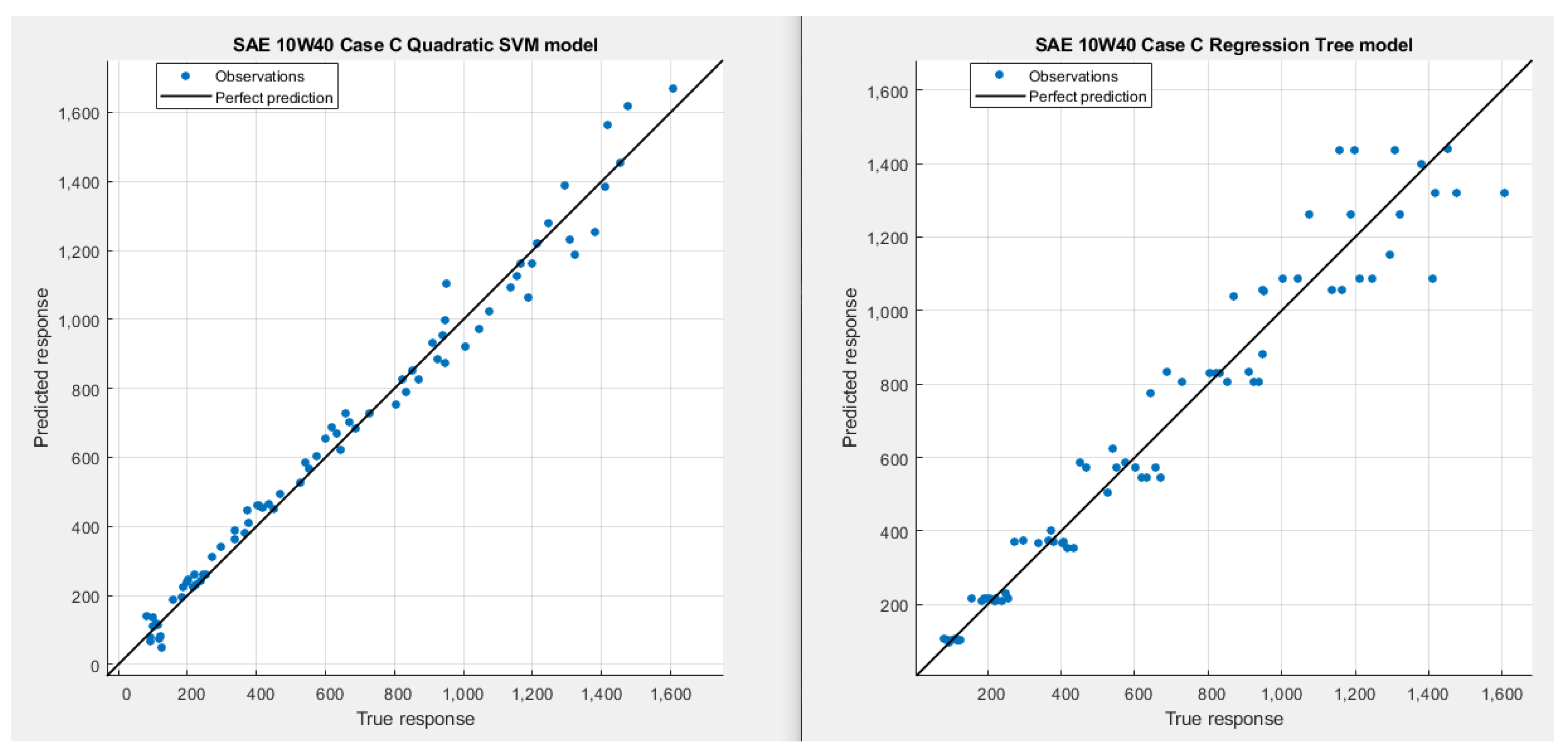
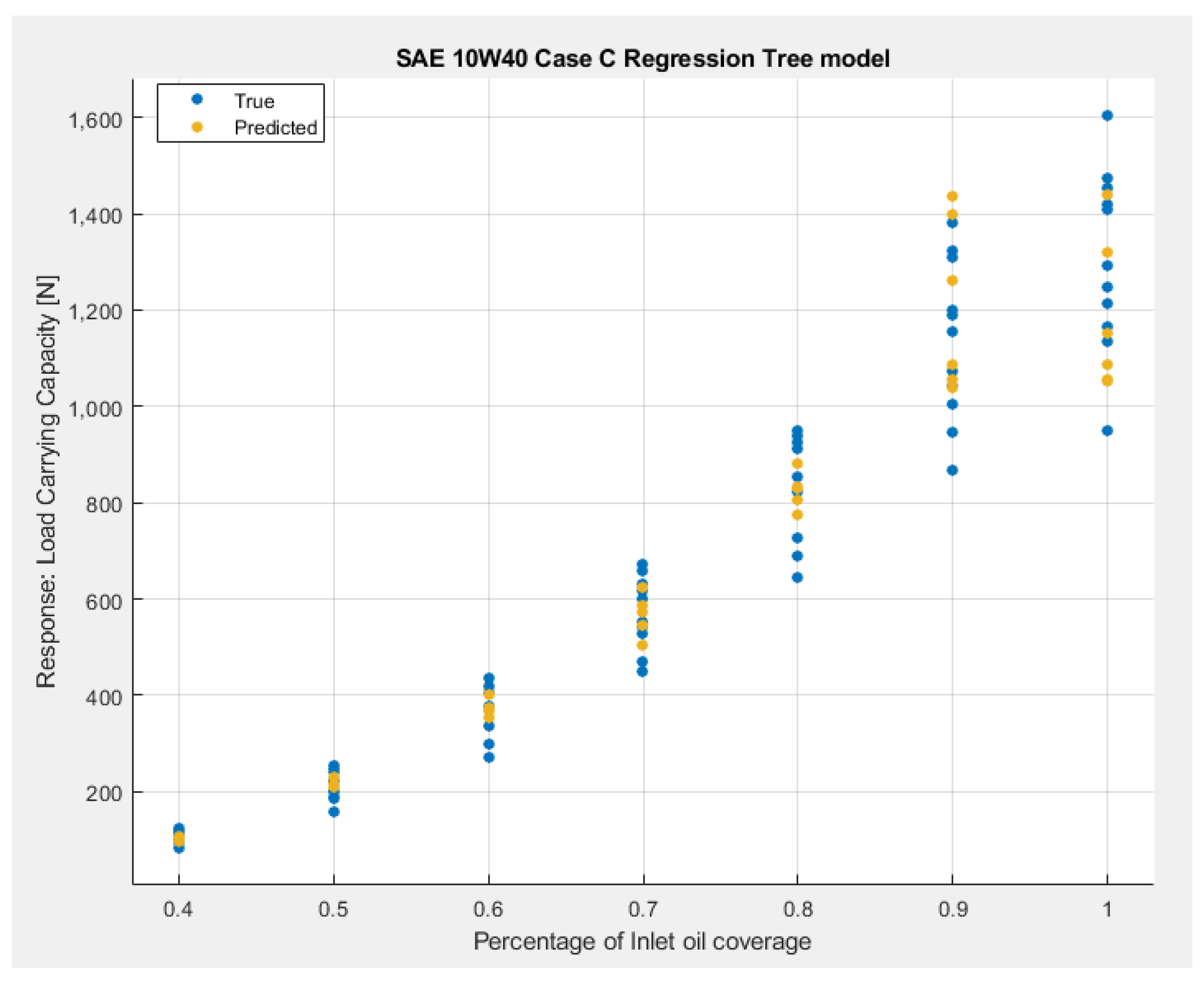
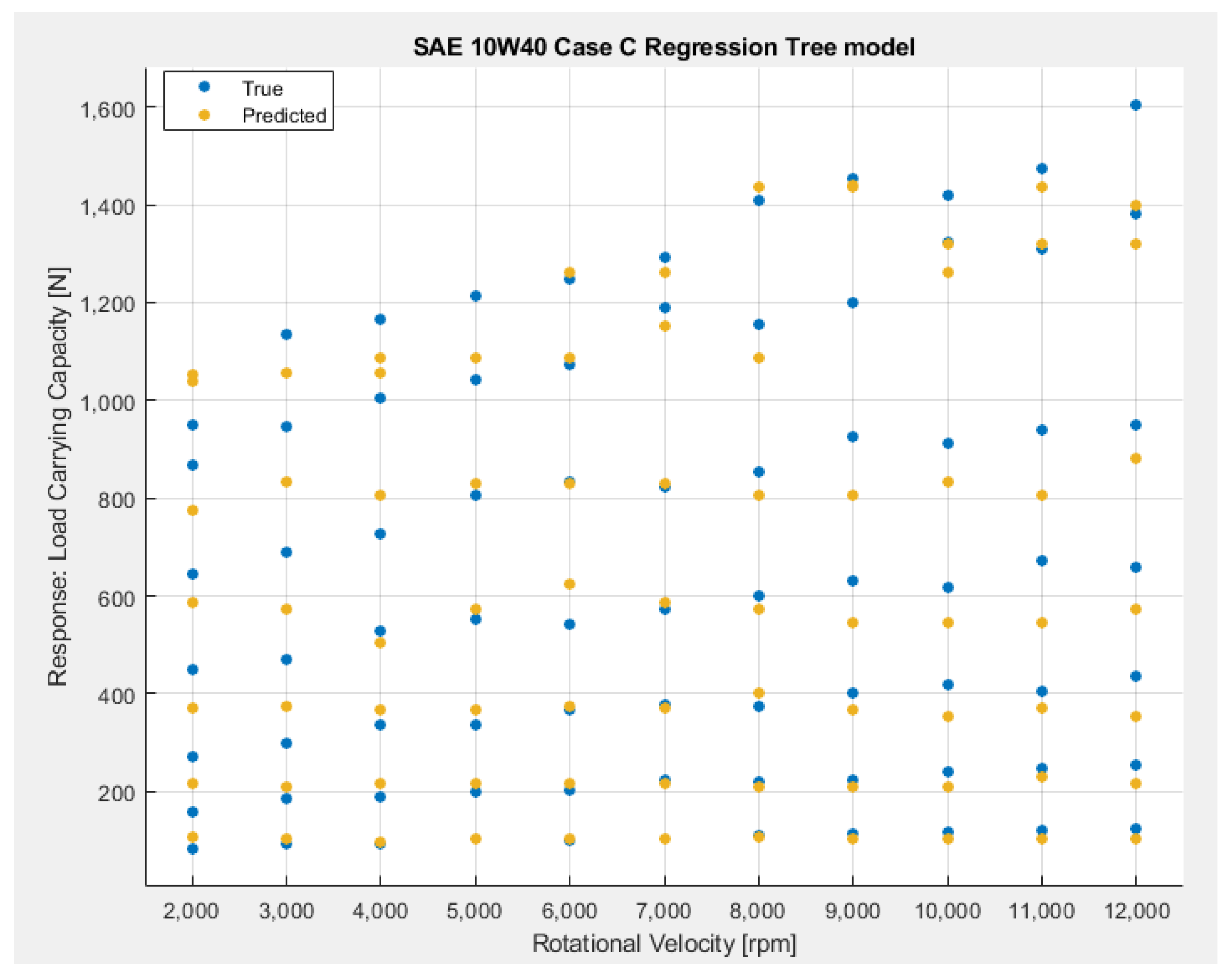
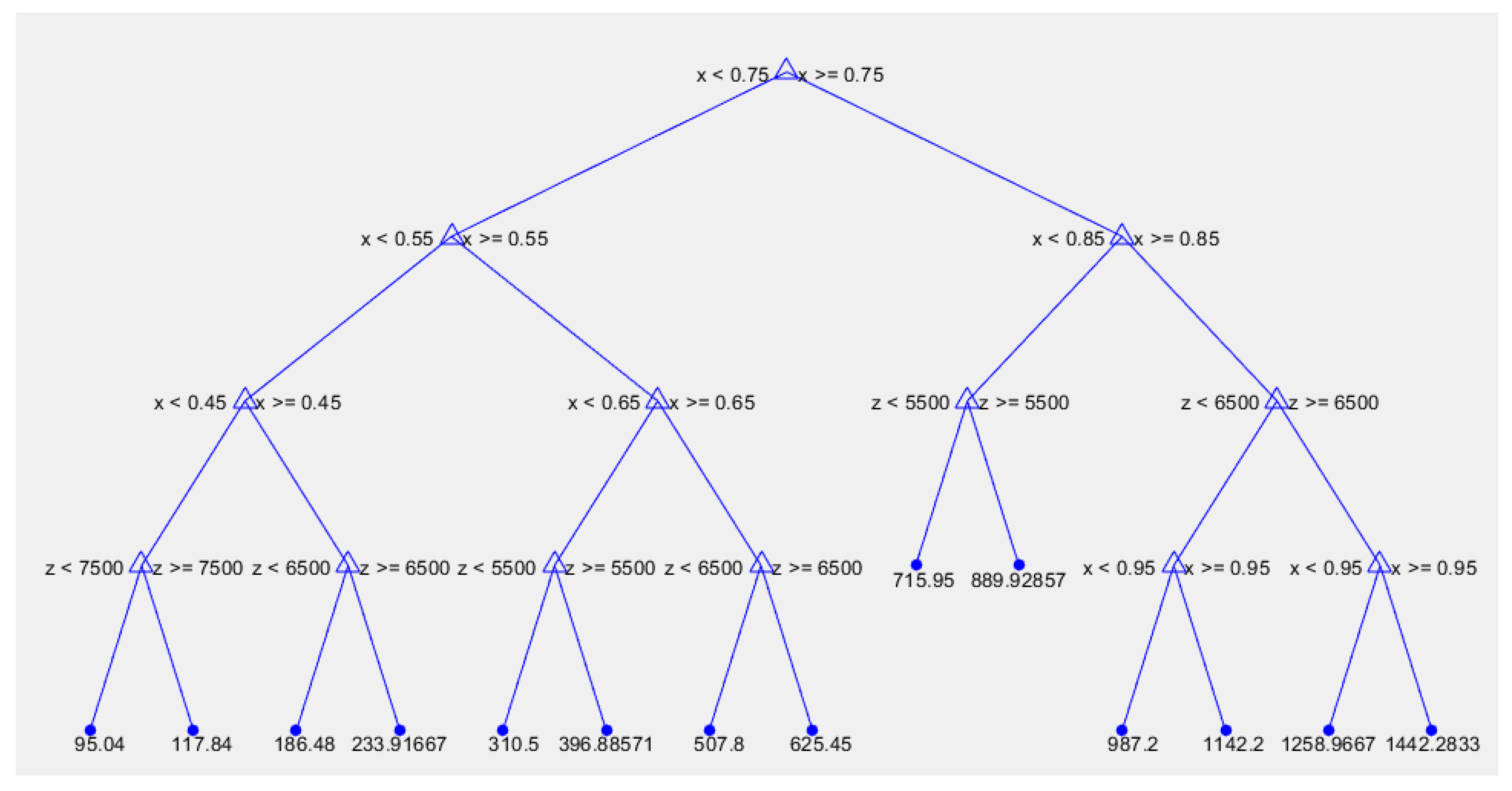
Taking a closer look at the results of case study C for the SAE 10W40, the lubricant with the optimum performance in terms of pad load-carrying capacity, one can notice that the Quadratic Polynomial Regression model has 99% accuracy in predicting the results. The Quadratic SVM model shows just 1% less accuracy with R2 = 0.98, while the Regression Tree model has an R2 = 0.95, which gives 4% less accuracy in load-carrying capacity prediction compared to the Quadratic Polynomial Regression model. Figure 13 is a graphical representation of the predicted versus the true response values for the Quadratic SVM and the Regression Tree models that were trained with Matlab’s Regression Learner tool. It is visually verified that the Quadratic SVM model has a better fit to the results compared to the Regression Tree model, since the observations (blue markers) are gathered very close to the prediction line compared to the Regression Tree model on the right, which shows a few observations with a higher deviation from the prediction line, mainly on the upper left corner. Figure 14 and Figure 15 (below) are the typical representation of the response plots for the SAE 10W40, case study C and Quadratic SVM model for each predictor. Similarly, Figure 16 and Figure 17 are the typical representations of the response plots for SAE 10W40, case study C and Regression Tree model. Finally, Figure 18 is the graphical representation of the Regression Tree machine-learning model for the lubricant SAE 10W40 and case study C- symmetrical, incomplete oil film profile.

4. Conclusions

In the current paper, the performance of a tilting pad thrust bearing was investigated in terms of the pad’s load-carrying capacity under various incomplete oil film profiles by combining numerical and machine-learning techniques. The 2-D Reynolds equation was solved numerically with the finite difference, central differences and method for three different lubricants: SAE 20, SAE 30 and SAE10W40. Three incomplete oil film profiles were studied, with the percentage of inlet oil coverage varying from 40% to 100%, and the rotational velocity of the rotor covering a range between 2000 and 12,000 rpm. In addition, the numerical data were used as input in order to train three machine-learning models: Quadratic Polynomial Regression, Quadratic SVM and Regression Trees. The conclusions of the investigation are summarized below:
As less oil covers the pad’s surface, the load-carrying capacity drops up to 93% for 40% of inlet oil coverage.
The load-carrying capacity of the pad is affected by the position of the oil film incompleteness. The lack of lubricant on the outer area of the pad, profile A, shows the worst load-carrying capacity results, while the case study C profile, with symmetrical lack of lubricant, presents up to 15% better performance.
From the studied lubricants, SAE 10W40 shows up to 135% better performance for the worst studied conditions of 12,000 rpm and 40% inlet oil coverage.
All the machine-learning models have a good accuracy in predicting the load-carrying capacity of the pad, since all R2 values are higher than 0.95.
Finally, the Quadratic Polynomial Regression ML model shows 1% better accuracy compared to the Quadratic SVM model, and 4% better accuracy when compared to the Regression Tree ML model.
All in all, the chosen machine-learning model that fits the needs of the current investigation in the best possible way is the Quadratic Polynomial Regression model. The lubricant that provides the pad with the optimum load-carrying capacity when facing incomplete oil film operating conditions is the SAE 10W40, and the worst case scenario is the lack of lubricant in the outer area of the pad’s surface.

Author Contributions

Conceptualization, writing—review and editing, P.G.N.; writing—original draft preparation, methodology, software and machine learning, K.P.K.; All authors carried out interpretations for the results. All authors have read and agreed to the published version of the manuscript.

Funding

This research received no external funding.

Institutional Review Board Statement

Not applicable.

Informed Consent Statement

Not applicable.

Data Availability Statement

Not applicable.

Conflicts of Interest

The authors declare no conflict of interest.

Nomenclature

A total area of bearing pads [m2]
B pad length in x-direction [m]
C 1 μ first viscosity coefficient—absolute temperature at which μ = μν (323 K)
C 2 μ second viscosity coefficient according to Sutherland’s law = 3800
C 3 μ third viscosity coefficient according to Sutherland’s law = 30,000
C n , s , w , e constants for each neighbor node
h film thickness [m]
h 0 , h 1 outlet, inlet film thickness [m]
h m i n minimum film thickness [m]: h m i n = min ( h 0 , h 1 )
k convergence ratio: k = ( h 1 h 0 ) / h 0
k e empirical constant = 0.8 [21]
L pad’s width in y-direction [m]
p absolute pressure [Pa]
P absolute nodal pressure [Pa]
q x , y lubricant flow [m3/h]
Q i n , o u t lubricant flow in inlet and outlet area of the pad [m3/h]
Q s r 1 , 2 lubricant outflow from the sides of the pad [m3/h]
T temperature [K]
U linear rotor velocity [m/s]
μ dynamic viscosity coefficient [Pas]
μ v nominal dynamic viscosity
x independent variable of length along pad’s width side [m]
ω rotational velocity [rpm]

References

  1. Ettles, C. The Development of a Generalized Computer Analysis for Sector Shaped Tilting Pad Thrust Bearings. ASLE Trans. 1976, 19, 153–163. [Google Scholar] [CrossRef]
  2. Markin, D.; McCarthy, D.; Glavatskih, S. A FEM approach to simulation of tilting-pad thrust bearing assemblies. Tribol. Int. 2003, 36, 807–814. [Google Scholar] [CrossRef]
  3. Dadouche, A.; Fillon, M.; Dmochowski, W. Performance of a Hydrodynamic Fixed Geometry Thrust Bearing: Comparison between Experimental Data and Numerical Results. Tribol. Trans. 2006, 49, 419–426. [Google Scholar] [CrossRef]
  4. Papadopoulos, C.I.; Kaiktsis, L.; Fillon, M. CFD Thermohydrodynamic Analysis of 3-D Sector-Pad Thrust Bearings with rectangular dimples. In Proceedings of the ASME Turbo Expo 2013: Turbine Technical Conference and Exposition, GT2013, San Antonio, TX, USA, 3–7 June 2013. [Google Scholar]
  5. Wasilczuk, M. Friction and Lubrication of Large Tilting-Pad Thrust Bearings. Lubricants 2015, 3, 164–180. [Google Scholar] [CrossRef]
  6. Fouflias, D.G.; Charitopoulos, A.G.; Papadopoulos, C.I.; Kaiktsis, L.; Fillon, M. Performance comparison between textured, pocket, and tapered-land sector-pad thrust bearings using computational fluid dynamics thermohydrodynamic analysis. Proc. Inst. Mech. Eng. Part J J. Eng. Tribol. 2014, 229, 376–397. [Google Scholar] [CrossRef]
  7. Gropper, D.; Harvey, T.J.; Wang, L. A numerical model for design and optimization of surface textures for tilting pad thrust bearings. Tribol. Int. 2018, 119, 190–207. [Google Scholar] [CrossRef]
  8. Katsaros, K.; Bompos, D.A.; Nikolakopoulos, P.G.; Theodossiades, S. Thermal-Hydrodynamic Behavior of Coated Pivoted Pad Thrust Bearings: Comparison between Babbitt, PTFE and DLC. Lubricants 2018, 6, 50. [Google Scholar] [CrossRef] [Green Version]
  9. Etsion, I.; Barkon, I. Analysis of a Hydrodynamic Thrust Bearing with Incomplete Film. J. Lubr. Technol. 1981, 103, 355–359. [Google Scholar] [CrossRef]
  10. Heshmat, H.; Artiles, A.; Pinkus, O. Paper IV(ii) Parametric study and optimization of starved thrust bearings. Tribol. Ser. 1987, 11, 105–112. [Google Scholar] [CrossRef]
  11. Artiles, A.; Heshmat, H. Analyis of Starved Thrust Bearings Including Temperature Effects. J. Tribol. 1987, 109, 395–401. [Google Scholar] [CrossRef]
  12. Moosavian, A.; Ahmadi, H.; Tabatabaeefar, A.; Khazaee, M. Comparison of Two Classifiers; K-Nearest Neighbor and Artificial Neural Network, for Fault Diagnosis on a Main Engine Journal-Bearing. Shock. Vib. 2013, 20, 263–272. [Google Scholar] [CrossRef]
  13. Alves, D.S.; Daniel, G.B.; de Castro, H.F.; Machado, T.H.; Cavalca, K.L.; Gecgel, O.; Dias, J.P.; Ekwaro-Osire, S. Uncertainty quantification in deep convolutional neural network diagnostics of journal bearings with ovalization fault. Mech. Mach. Theory 2020, 149, 103835. [Google Scholar] [CrossRef]
  14. Poddar, S.; Tandon, N. Classification and detection of cavitation, particle contamination and oil starvation in journal bearing through machine learning approach using acoustic emission signals. Proc. Inst. Mech. Eng. Part J J. Eng. Tribol. 2021, 235, 2137–2143. [Google Scholar] [CrossRef]
  15. Lorza, R.L.; Garcia, R.E.; Martinez, R.F.; Cueva, M.I.; MacDonald, B.J. Using the finite element method and data mining techniques as an alternative method to determine the maximum load capacity in tapered roller bearings. J. Appl. Log. 2016, 24, 4–14. [Google Scholar] [CrossRef]
  16. Katsaros, K.P.; Nikolakopoulos, P.G. On the tilting-pad thrust bearings hydrodynamic lubrication under combined numerical and machine learning techniques. Lubr. Sci. 2021, 33, 153–170. [Google Scholar] [CrossRef]
  17. Moschopoulos, M.; Rossopoulos, G.N.; Papadopoulos, C.I. Journal Bearing Performance Prediction Using Machine Learning and Octave-Band Signal Analysis of Sound and Vibration Measurements. Pol. Marit. Res. 2021, 28, 137–149. [Google Scholar] [CrossRef]
  18. Zavos, A.; Katsaros, K.P.; Nikolakopoulos, P.G. Optimum Selection of Coated Piston Rings and Thrust Bearings in Mixed Lubrication for Different Lubricants Using Machine Learning. Coatings 2022, 12, 704. [Google Scholar] [CrossRef]
  19. Aurelian, F.; Patrick, M.; Mohamed, H. Wall slip effects in (elasto) hydrodynamic journal bearings. Tribol. Int. 2011, 44, 868–877. [Google Scholar] [CrossRef]
  20. Tala-Ighil, N.; Fillon, M. A numerical investigation of both thermal and texturing surface effects on the journal bearings static characteristics. Tribol. Int. 2015, 90, 228–239. [Google Scholar] [CrossRef]
  21. Stachowiak, G.W.; Batchelor, A.W. Thermal Effects in Bearings. In Engineering Tribology; Paragraph 4.6; Butterworth-Heinemann Elsevier Ltd.: Oxford, UK, 2014; Chapter 4. [Google Scholar]
  22. Bielec, M.K.; Leopard, A.J. Paper 13: Tilting Pad Thrust Bearings: Factors Affecting Performance and Improvements with Directed Lubrication. Proc. Inst. Mech. Eng. Conf. Proc. 1969, 184, 93–102. [Google Scholar] [CrossRef] [Green Version]
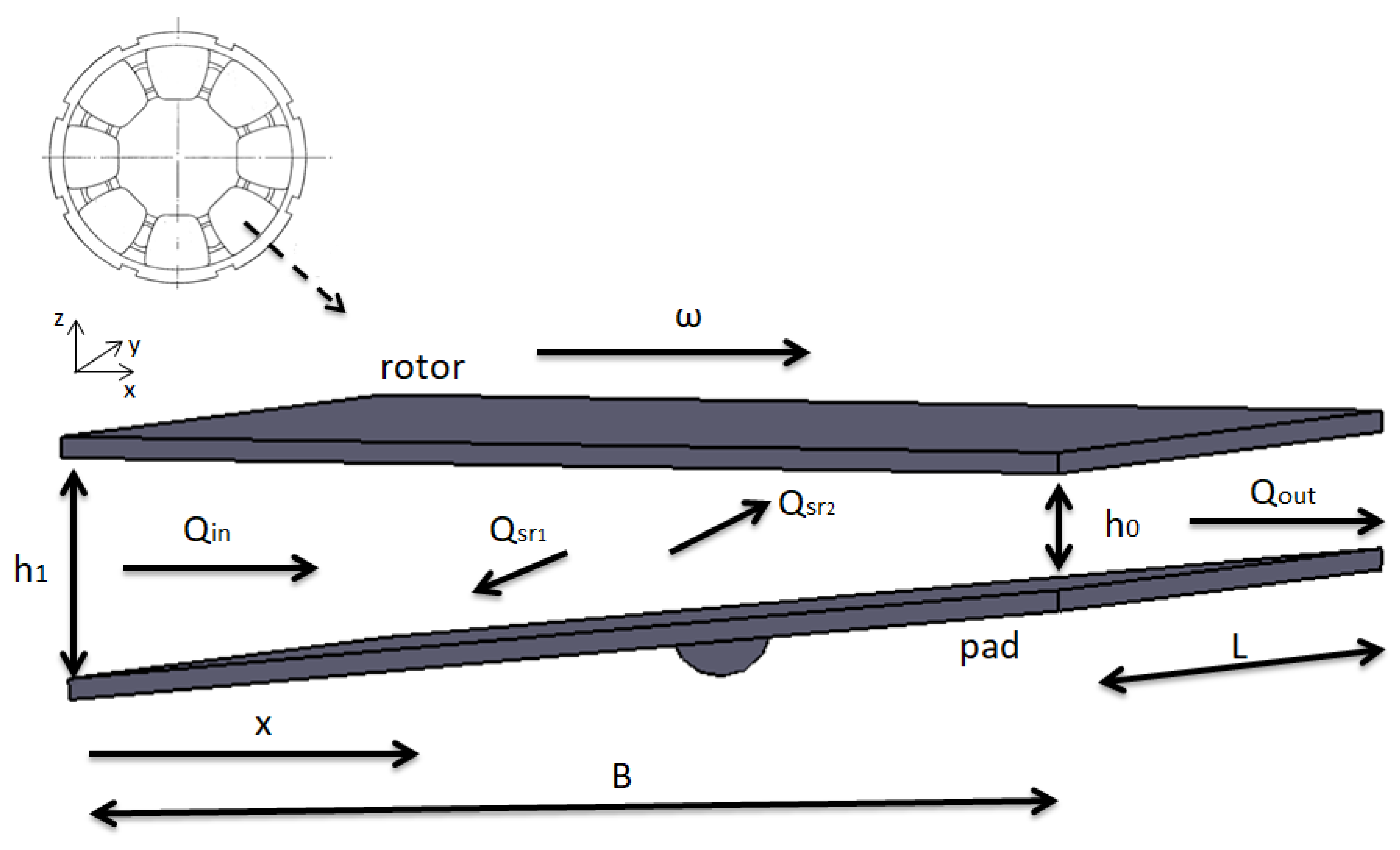
Figure 1. Pivoted pad thrust bearing schematic.
Lubricants 11 00113 g001
Figure 2. Dynamic Viscosity variation according to Temperature for SAE 20, SAE 30 and SAE 10W40.
Lubricants 11 00113 g002
Figure 3. Finite Difference-Central Differences Computation Grid.
Lubricants 11 00113 g003
Figure 4. Computation grid, along with the incomplete oil film areas.
Lubricants 11 00113 g004
Figure 5. Numerical and Experimental Specific Pad Load- Data Validation.
Lubricants 11 00113 g005
Figure 6. Typical pad’s pressure distribution for the Case A incomplete oil film profile at 60% oil film coverage for the inlet of the pad.
Lubricants 11 00113 g006
Figure 7. Typical pad’s pressure distribution for the Case B incomplete oil film profile at 60% oil film coverage for the inlet of the pad.
Lubricants 11 00113 g007
Figure 8. Typical pad’s pressure distribution for the Case C incomplete oil film profile at 60% oil film coverage for the inlet of the pad.
Lubricants 11 00113 g008
Figure 9. Quadratic Polynomial Regression model of SAE30 for all the incomplete oil film profiles. Load-carrying capacity according to percentage of inlet oil coverage and rotational velocity.
Lubricants 11 00113 g009
Figure 10. Quadratic Polynomial Regression model of SAE10W40 for all the incomplete oil film profiles. Load-carrying capacity according to percentage of inlet oil coverage and rotational velocity.
Lubricants 11 00113 g010
Figure 11. Quadratic Polynomial Regression model of SAE 20 for all the incomplete oil film profiles. Load-carrying capacity according to percentage of inlet oil coverage and rotational velocity.
Lubricants 11 00113 g011
Figure 12. Quadratic Polynomial Regression model of incomplete oil film profile C for all the studied lubricants. Load-carrying capacity according to percentage of inlet oil coverage and rotational velocity.
Lubricants 11 00113 g012
Figure 13. SVM model VS Regression Tree model- True and Prediction response plots for SAE 10W40, case C.
Lubricants 11 00113 g013
Figure 14. Typical response plot of the pad’s inlet oil coverage and load-carrying capacity for the Quadratic SVM model, SAE 10W40, case C profile.
Lubricants 11 00113 g014
Figure 15. Typical response plot of the rotational velocity and load-carrying capacity for the Quadratic SVM model, SAE 10W40, case C profile.
Lubricants 11 00113 g015
Figure 16. Typical response plot of the pad’s inlet oil coverage and load-carrying capacity for the Regression Tree model, SAE 10W40, case C profile.
Lubricants 11 00113 g016
Figure 17. Typical response plot of the pad’s rotational velocity and load-carrying capacity for the Regression Tree model, SAE 10W40, case C profile.
Lubricants 11 00113 g017
Figure 18. Graphical representation of the Regression Tree model for the SAE 10W40, case C incomplete oil film profile.
Lubricants 11 00113 g018
Table 1. Input parameters for the simulations.
Pad’s Length32mm
Pad’s Width28mm
Pad’s Outer Radious62mm
Pad’s Inclination0.1
Pad’s Pivotcenter
Rotational Velocity2000–12,000rpm
Percentage of Inlet Oil Coverage0.4–1
SAE 20 dynamic viscosity @50 °C0.033Pasec
SAE 30 dynamic viscosity @50 °C0.046Pasec
SAE 10W40 dynamic viscosity @50 °C0.054Pasec
SAE 20 density @40 °C861Kg/m3
SAE 20 specific heat capacity2021J/kgK
SAE 30 density @40 °C869Kg/m3
SAE 30 specific heat capacity1950J/kgK
SAE 10W40 density @40 °C851Kg/m3
SAE 10W40 specific heat capacity1980J/kgK
Lubricant’s Inlet Temperature323K
Table 2. Quadratic Polynomial Regression models.
Case StudyML ModelR2
SAE 30 Case A y = 139.4 891 x 1 0.016 x 2 + 1577 x 1 2 + 0.075 x 1 x 2 0.1 × 10 5 x 2 2 0.99
SAE 30 Case B y = 5.1 405.3 x 1 0.021 x 2 + 1240.7 x 1 2 + 0.08 x 1 x 2 0.8 × 10 6 x 2 2 0.99
SAE 30 Case C y = 57.7 189.7 x 1 0.02 x 2 + 1087.3 x 1 2 + 0.08 x 1 x 2 0.8 × 10 6 x 2 2 0.99
SAE 10W40 Case A y = 172.3 1035.4 x 1 0.023 x 2 + 1792.5 x 1 2 + 0.09 x 1 x 2 0.1 × 10 5 x 2 2 0.99
SAE 10W40 Case B y = 101.7 748.3 x 1 0.026 x 2 + 1593.4 x 1 2 + 0.09 x 1 x 2 0.8 × 10 6 x 2 2 0.99
SAE 10W40 Case C y = 23.1 496.5 x 1 0.023 x 2 + 1419.2 x 1 2 + 0.09 x 2 0.9 × 10 6 x 2 2 0.99
SAE 20 Case A y = 80.3 729.3 x 1 0.01 x 2 + 1409.1 x 1 2 + 0.07 x 1 x 2 0.1 × 10 5 x 2 2 0.99
SAE 20 Case B y = 38.7 325.4 x 1 0.009 x 2 + 1127.1 x 1 2 + 0.07 x 1 x 2 0.1 × 10 5 x 2 2 0.99
SAE 20 Case C y = 909 1418.2 x 1 0.09 x 2 + 9977.2 x 1 2 + 0.7 x 1 x 2 0.1 × 10 4 x 2 2 0.99
Table 3. Quadratic SVM and Regression Tree models and their corresponding R2.
Case StudyR2
SAE 30 Quadratic SVM ML model0.98
SAE 30 Regression Tree ML model0.95
SAE 10W40 Quadratic SVM ML model0.98
SAE 10W40 Regression Tree ML model0.95
SAE 20 Quadratic SVM ML model0.98
SAE 20 Regression Tree ML model0.95
Disclaimer/Publisher’s Note: The statements, opinions and data contained in all publications are solely those of the individual author(s) and contributor(s) and not of MDPI and/or the editor(s). MDPI and/or the editor(s) disclaim responsibility for any injury to people or property resulting from any ideas, methods, instructions or products referred to in the content.