Reconstruction and Intelligent Evaluation of Three-Dimensional Texture of Stone Matrix Asphalt-13 Pavement for Skid Resistance


Abstract
:1. Introduction
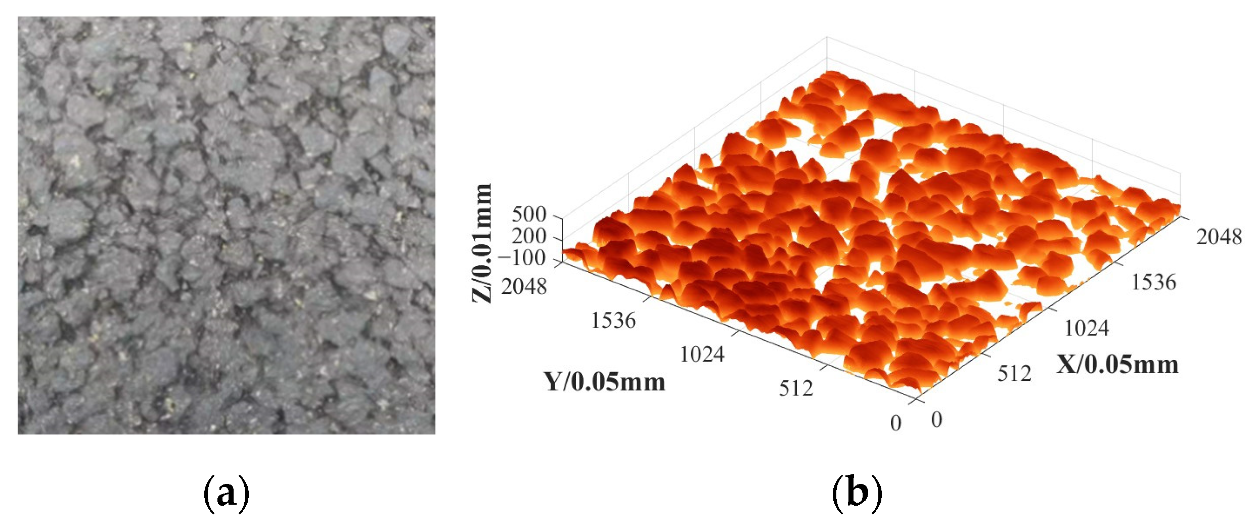
2. SMA-13 Asphalt Pavement Data Acquisition
2.1. Technical Performance Index of Raw Materials
2.2. SMA-13 Asphalt Mixture Grading
2.3. Data Acquisition
3. Three-Dimensional Reconstruction of Asphalt Pavement Texture
3.1. Slope Correction
3.2. Noise Reduction Optimization and Texture Reconstruction
3.3. Macro- and Microtexture Separation
4. Intelligent Evaluation of Asphalt Pavement Skid Resistance
4.1. Asphalt Pavement Three-Dimensional Texture Characterization Index
- (1)
- Mean Profile Depth (MPD)
- (2)
- Skewness (Rsk)
- (3)
- Kurtosis (Rku)
- (4)
- Two-Point Slope Elevation Difference (SV2pts)
- (5)
- Contour Arithmetic Mean Deviation (Ra)
- (6)
- Root-Mean-Square Roughness (RMS)
4.2. Intelligent Evaluation Method of Asphalt Pavement Anti-Skid Performance
- (1)
- Histogram-based Learning
- (2)
- Leaf-wise Growth
- (3)
- Gradient-based One-Side Sampling (GOSS):
- (4)
- Exclusive Feature Bundling (EFB):
4.3. Established Anti-Skid Intelligent Evaluation Model Based on LightGBM
- Traversing each feature and selecting split points for each feature. For continuous features, this involves selecting a threshold value for splitting, while for discrete features, each distinct value is selected as a split point.
- At each split point, the reduction in model error after splitting using the feature is calculated, usually using metrics such as information gain or the reduction in Gini impurity.
- After selecting the split point for each feature, the error reduction at different split points is summarized to obtain the overall contribution of the feature to the model.
- Ultimately, the importance of each feature can be ranked through normalization.
5. Conclusions
- The high-precision 3D texture scanning equipment effectively captured the surface texture structure of asphalt concrete pavement.
- Employing the least-squares method for slope modification and wavelet transform for noise reduction enabled successful three-dimensional texture reconstruction of the pavement.
- The LightGBM pavement skid resistance intelligent assessment model combines texture characteristics and friction coefficients, and Rku and MPD are still effective indicators for evaluating skid resistance, scoring the highest in this model. This indicates that it can effectively reflect the changes in road surface contact texture caused by long-term vehicle wear.
- The different effects of Micro_Rku and Macro_Rku on the coefficient of friction emphasize the different effects of macrotexture and microtexture on the anti-skid performance of pavements, and it is also found that the macrotexture features of pavements have a greater effect on the coefficient of friction BPN than the microtexture features of pavements in this model.
- Comparative analyses revealed the superiority of the LightGBM model over traditional multivariate linear and random forest models, attaining the training set R2 of 0.948, and the testing set R2 of 0.842.
Author Contributions
Funding
Data Availability Statement
Conflicts of Interest
References
- Li, H. Research on Network Level Decision-Making of Highway Asphalt Pavement Maintenance Based on Matter-Element Model. Ph.D. Thesis, Southeast University, Nanjing, China, 2017. [Google Scholar]
- Zhu, H.; Liao, Y. Present Situations of Research on Anti-skid Property of Asphalt Pavement. Highway 2018, 63, 35–46. [Google Scholar]
- Ding, S.H.; Zhan, Y.; Yang, E.H.; Wang, C.P. MTD measurement of asphalt pavement based on high precision laser section elevation. J. Southeast Univ. (Nat. Sci. Ed.) 2020, 50, 137–142. [Google Scholar]
- Lin, L. Numerical Relation Study on Three-Dimensional Texture Structure and Skid Resistance of Road Surface. Master’s Thesis, Xinjiang University, Xinjiang, China, 2019. [Google Scholar]
- Liu, Q.; Shalaby, A. Relating concrete pavement noise and friction to three-dimensional texture parameters. Int. J. Pavement Eng. 2015, 18, 450–458. [Google Scholar] [CrossRef]
- Song, H. Research on the Influence of Macro and Micro Texture of Asphalt Pavement on Friction Coefficient. Transp. Sci. Technol. 2022, 3, 22–26. [Google Scholar]
- Jiang, T.H.; Ren, W.Y.; Dong, Y.S. Precise Representation of Macro-Texture of Pavement and Effect on Anti-Skidding Performance. J. Munic. Technol. 2022, 40, 1–7+24. [Google Scholar] [CrossRef]
- Huang, X.M.; Zheng, B.S. Research Status and Progress for Skid Resistance Performance of Asphalt Pavements. China J. Highw. Transp. 2019, 32, 32–49. [Google Scholar] [CrossRef]
- Sun, C.Y.; Han, Y.X.; Hu, Y.J.; Gao, S.; Weng, Y.H. Evaluation of Skid Resistance of Asphalt Pavement Based on IGWO-XGBoost Fusion Model. Comput. Syst. Appl. 2023, 32, 1–11. [Google Scholar] [CrossRef]
- Li, Q.J.; Zhan, Y.; Yang, G.; Wang, K.C.P. Pavement skid resistance evaluation based on 3D areal texture characterization. J. Southeast Univ. (Nat. Sci. Ed.) 2020, 50, 667–676. [Google Scholar]
- Zhan, Y.; Deng, Q.; Luo, Z.; Liu, C.; Zhang, A.; Qiu, Y. Research on GBDT-based skid resistance perception model for asphalt pavement. China Civ. Eng. J. 2023, 56, 121–132. [Google Scholar] [CrossRef]
- Zhang, R.; Hu, J. Production performance forecasting method based on multivariate timeseries and vector autoregressive machine learning model for waterflooding reservoirs. Pet. Explor. Dev. 2021, 48, 175–184. [Google Scholar] [CrossRef]
- Kou, W.; Dong, H.; Zhou, M. A hybrid wavelet-machine learning approach for prediction of equivalent thermal conductivity properties of hybrid composites. Acta Phys. Sin. 2021, 70, 63–74. [Google Scholar] [CrossRef]
- Liu, C.; Li, J.; Gao, J.; Yuan, D.; Gao, Z.; Chen, Z. Three-dimensional texture measurement using deep learning and multi-view pavement images. Measurement 2021, 172, 108828. [Google Scholar] [CrossRef]
- Hu, Y.J. Multi-Scale Texture Feature Extraction and Skid Resistance Performance Evaluation of Asphalt Pavement Based on Point Cloud Data. Ph.D. Thesis, Chang’an University, Xi’an, China, 2023. [Google Scholar]
- Deng, Q. Study on Intelligent Pavement Friction EvaluationModel and Maintenance Decision for Optimized Skid Resistance. Master’s Thesis, Southwest Jiaotong University, Chengdu, China, 2022. [Google Scholar]
- Liu, C. Resistance and Decay Prediction of Asphalt Pavement Skid Ensemble Learning Models for Non-Contact Evaluation. Master’s Thesis, Southwest Jiaotong University, Chengdu, China, 2022. [Google Scholar]
- JTG E60-2008; Field Test Methods of Subgrade and Pavement for Highway Engineering; Volume. Standardization Administration of the People’s Republic of China: Beijing, China, 2008.
- Ren, W. Study on the Abrasion Characteristic of Surface Textureand Its Effect on Noise for Asphalt Pavements. Master’s Thesis, Chang’an University, Xi’an, China, 2019. [Google Scholar]
- Li, W.; Lin, C.; Liao, H. Simulation Study and Evaluation of Random Effect-Expectation Maximization Regression Tree Model. Chin. J. Health Stat. 2019, 36, 665–668+673. [Google Scholar]
- Wei, W.; Du, Y.; Dong, A.; Qin, D.; Zhu, T. An Analysis of Factors Affecting Injury of Electric Two-wheeler Riders Based on CIDAS Data and Ensemble Learning. J. Transp. Inf. Saf. 2022, 40, 45–52. [Google Scholar]
- Yoon, H.I.; Lee, H.; Yang, J.-S. Predicting Models for Plant Metabolites Based on PLSR, AdaBoost, XGBoost, and LightGBM Algorithms Using Hyperspectral Imaging of Brassica juncea. Agriculture 2023, 13, 1477. [Google Scholar] [CrossRef]
- Bapatla, S.; Harikiran, J. LuNet-LightGBM: An Effective Hybrid Approach for Lesion Segmentation and DR Grading. Comput. Syst. Sci. Eng. 2023, 46, 597–617. [Google Scholar] [CrossRef]
- Wang, D.-N.; Li, L.; Zhao, D. Corporate finance risk prediction based on LightGBM. Inf. Sci. 2022, 602, 259–268. [Google Scholar] [CrossRef]
- Zhu, X.; Yin, Q.; Zhao, F. Ship speed prediction model based on LightGBM. J. Dalian Marit. Univ. 2023, 49, 56–65. [Google Scholar]
- Ke, G.; Meng, Q.; Finley, T.; Wang, T.; Chen, W.; Ma, W.; Ye, Q.; Liu, T.-Y. Lightgbm: A highly efficient gradient boosting decision tree. Adv. Neural Inf. Process. Syst. 2017, 30, 3149–3157. [Google Scholar]


| Test Items | Units | Test Results | Technical Requirements | |
|---|---|---|---|---|
| Needle penetration (25 °C; 100 g, 5 s) | mm | 57 | 40–60 | |
| Softening point | °C | 78 | ≥60 | |
| Ductility (5 °C, 5 cm/min) | cm | 29 | ≥20 | |
| 135 °C dynamic viscosities | pa·s | 2.28 | ≤3 | |
| Elastic recovery 25 °C | % | 82 | ≥75 | |
| Film heating experiment | Mass loss | % | −0.1 | ≤±1 |
| Needle penetration ratio 25 °C | % | 80 | ≥65 | |
| 5 °C elongations | cm | 17 | ≥15 | |
| Test Items | Units | Test Results | Technical Requirements |
|---|---|---|---|
| Crush value | % | 15.8 | ≤30 |
| Water absorption | % | 0.57 | ≤3 |
| Needle flake particle content | % | 11.9 | ≤20 |
| Los Angeles wear value | % | 18.6 | ≤35 |
| Test Items | Units | Test Results | Technical Requirements |
|---|---|---|---|
| Sand equivalent | % | 65 | >50 |
| Mud content (<0.075 mm portion) | % | 1.8 | ≤3 |
| Test Items | Units | Detection Result | Technical Requirements | |
|---|---|---|---|---|
| Moisture content | % | 0.7 | ≤1 | |
| Apparent relative density | g/m3 | 2.712 | ≥2.5 | |
| Percentage through the sieve | 0.6 mm | % | 100 | 100 |
| 0.15 mm | % | 95.7 | 90–100 | |
| 0.075 mm | % | 88.6 | 75–100 | |
| Appearance | No clumps | |||
| Gradation | Percentage through Different Screen Size (mm)/% | ||||||||||
|---|---|---|---|---|---|---|---|---|---|---|---|
| 16 | 13.2 | 9.5 | 4.75 | 2.36 | 1.18 | 0.6 | 0.3 | 0.15 | 0.075 | ||
| SMA-13 grading range | Upper limit | 100 | 100 | 75 | 31 | 26 | 24 | 20 | 16 | 15 | 12 |
| Median | 100 | 95 | 62.5 | 27 | 20.5 | 19 | 16 | 13 | 12 | 10 | |
| Lower limit | 100 | 90 | 50 | 20 | 15 | 14 | 12 | 10 | 9 | 8 | |
| T/°C | 0 | 5 | 10 | 15 | 20 | 25 | 30 | 35 | 40 |
| ΔBPN | −6.0 | −4.0 | −3.0 | −1.0 | 0 | 2.0 | 3.0 | 5.0 | 7.0 |
| Models | ML | RF | LightGBM | |
|---|---|---|---|---|
| R2 | Training | 0.712 | 0.835 | 0.948 |
| Testing | 0.689 | 0.761 | 0.842 | |
Disclaimer/Publisher’s Note: The statements, opinions and data contained in all publications are solely those of the individual author(s) and contributor(s) and not of MDPI and/or the editor(s). MDPI and/or the editor(s) disclaim responsibility for any injury to people or property resulting from any ideas, methods, instructions or products referred to in the content. |
© 2023 by the authors. Licensee MDPI, Basel, Switzerland. This article is an open access article distributed under the terms and conditions of the Creative Commons Attribution (CC BY) license (https://creativecommons.org/licenses/by/4.0/).
Share and Cite
Dai, G.; Luo, Z.; Chen, M.; Zhan, Y.; Ai, C. Reconstruction and Intelligent Evaluation of Three-Dimensional Texture of Stone Matrix Asphalt-13 Pavement for Skid Resistance. Lubricants 2023, 11, 535. https://doi.org/10.3390/lubricants11120535
Dai G, Luo Z, Chen M, Zhan Y, Ai C. Reconstruction and Intelligent Evaluation of Three-Dimensional Texture of Stone Matrix Asphalt-13 Pavement for Skid Resistance. Lubricants. 2023; 11(12):535. https://doi.org/10.3390/lubricants11120535
Chicago/Turabian StyleDai, Gang, Zhiwei Luo, Mingkai Chen, You Zhan, and Changfa Ai. 2023. "Reconstruction and Intelligent Evaluation of Three-Dimensional Texture of Stone Matrix Asphalt-13 Pavement for Skid Resistance" Lubricants 11, no. 12: 535. https://doi.org/10.3390/lubricants11120535
APA StyleDai, G., Luo, Z., Chen, M., Zhan, Y., & Ai, C. (2023). Reconstruction and Intelligent Evaluation of Three-Dimensional Texture of Stone Matrix Asphalt-13 Pavement for Skid Resistance. Lubricants, 11(12), 535. https://doi.org/10.3390/lubricants11120535