Prediction of Remaining Service Life of Rolling Bearings Based on Convolutional and Bidirectional Long- and Short-Term Memory Neural Networks

Abstract

Predicting the remaining useful life (RUL) of a bearing can prevent sudden downtime of rotating machinery, thereby improving economic efficiency and protecting human safety. Two important steps in RUL prediction are the construction of a health indicator (HI) and the prediction of life. Traditional methods simply use the time-series characteristics of the vibration signal, for example, using root mean square (RMS) as HI, but this HI does not reflect the true degradation of the bearing. Meanwhile, existing prediction models often cannot consider both the time and space characteristics of the signal, thus limiting prediction accuracy. To address the above problems, in this study, wavelet packet transform (DWPT) and kernel principal component analysis (KPCA) were combined to extract HI from the original vibration signal. Then, a CNN-BiLSTM (convolutional and bidirectional long- and short-term memory) prediction network with root mean square as input and HI as output was constructed by combining convolutional neural network (CNN) and bi-directional long- and short-term memory neural network (BiLSTM). The network improved prediction accuracy by considering the temporal and spatial characteristics of the input signal. Experimental results on the PHM2012 dataset showed that the method proposed in this paper outperformed existing methods.

1. Introduction

Bearing is a key component in rotating machinery, known as the joint of machinery, and its failure may lead to downtime of industrial production or even cause casualties [1]. According to a survey, rolling bearing failure is one of the most important factors of rotating machinery failure, accounting for 45–55% of cases [2]. A reasonable and effective bearing remaining useful life prediction (RUL) method can help technicians develop maintenance plans for predictive maintenance [3]. Therefore, it is important to predict the remaining service life of bearings to avoid accidents and reduce economic losses [4].

Generally speaking, methods for RUL prediction of bearings fall into two main categories: model-based (physical/mathematical) methods [5,6] and data-driven methods [7]. Wang et al. [8] proposed a mechanical state prediction method based on a probabilistic model with particle filters, which was successfully used for the state prediction of wind power bearings. El-Tawil et al. [9] developed a method based on a nonlinear damage law to determine the RUL of the system. Ma et al. [5] analyzed the interaction between various parts of the bearing by modeling the angle of relative sliding velocity between the rolling element and the bearing raceway and the bearing dynamics. However, model-based methods require complex physical or mathematical models, which require researchers with extensive knowledge base and are often difficult to develop due to complex working conditions [10].

With the development of sensor technology and computer technology, data-driven methods based on data have been developed [11]. As a data-driven method, deep learning can learn the bearing degradation trend spontaneously from sensor data and establish the mapping relationship between data and bearing health status with remarkable application [12]. Deep-learning-based RUL prediction methods are mainly divided into steps such as data acquisition, health factor (HI) construction, and remaining service life prediction [13]. Liu et al. [14] proposed a rolling bearing RUL prediction method based on regularized LSTM networks and verified the advantages of the method with the dataset of PRONOSTIA platform [15]. Ning et al. [16] first performed feature screening of signals and then predicted the remaining service life of bearings using RNN models. Network models such as RNN and LSTM tend to ignore spatial features, although they can learn the degradation trend and temporal characteristics of bearings from the data [17]. Wang et al. [18] used 1d-CNN to process fused signals and learn fault features using the powerful feature extraction capability of the network. However, a single CNN network tends to ignore the temporal features of the data and is unable to learn signal features at multiple scales [19]. HI can reflect the degradation trend of bearings, and it is critical to obtain excellent HI labels for training prediction models [20]. For example, Zhang et al. [21] used the time-domain feature RMS of the vibration signal as the main performance degradation indicator. Singleton et al. [22] used the variance of the vibration signal as HI. Zhang et al. [23] used the kurtosis of the vibration signal after band-pass filtering as HI. In the literature [24], the ratio of current life to total life of the bearing is used as HI of the bearing. However, HI constructed by the above methods cannot fully describe the bearing degradation trend. Because the bearing signal is nonlinear, we can pay attention to the transient changes of the signal by analyzing the signal with different resolutions in time–frequency domain. Time–frequency analysis technology DWPT is often used in the analysis of bearing vibration signals [25].

In response to the above problems, a new method for HI and RUL prediction of rolling bearings is proposed in this paper. Firstly, discrete wavelet packet transform (DWPT) was performed on the time-domain vibration signal to extract RMS features from the obtained sub-bands, and the HI was then obtained by fusing the RMS of each sub-band through kernel principal component analysis (KPCA). Based on this, the convolutional bidirectional long- and short-term memory neural network (CNN-BiLSTM) was proposed for lifetime prediction. Finally, the feasibility of the method was verified by bearing experimental data. The main contributions are as follows.

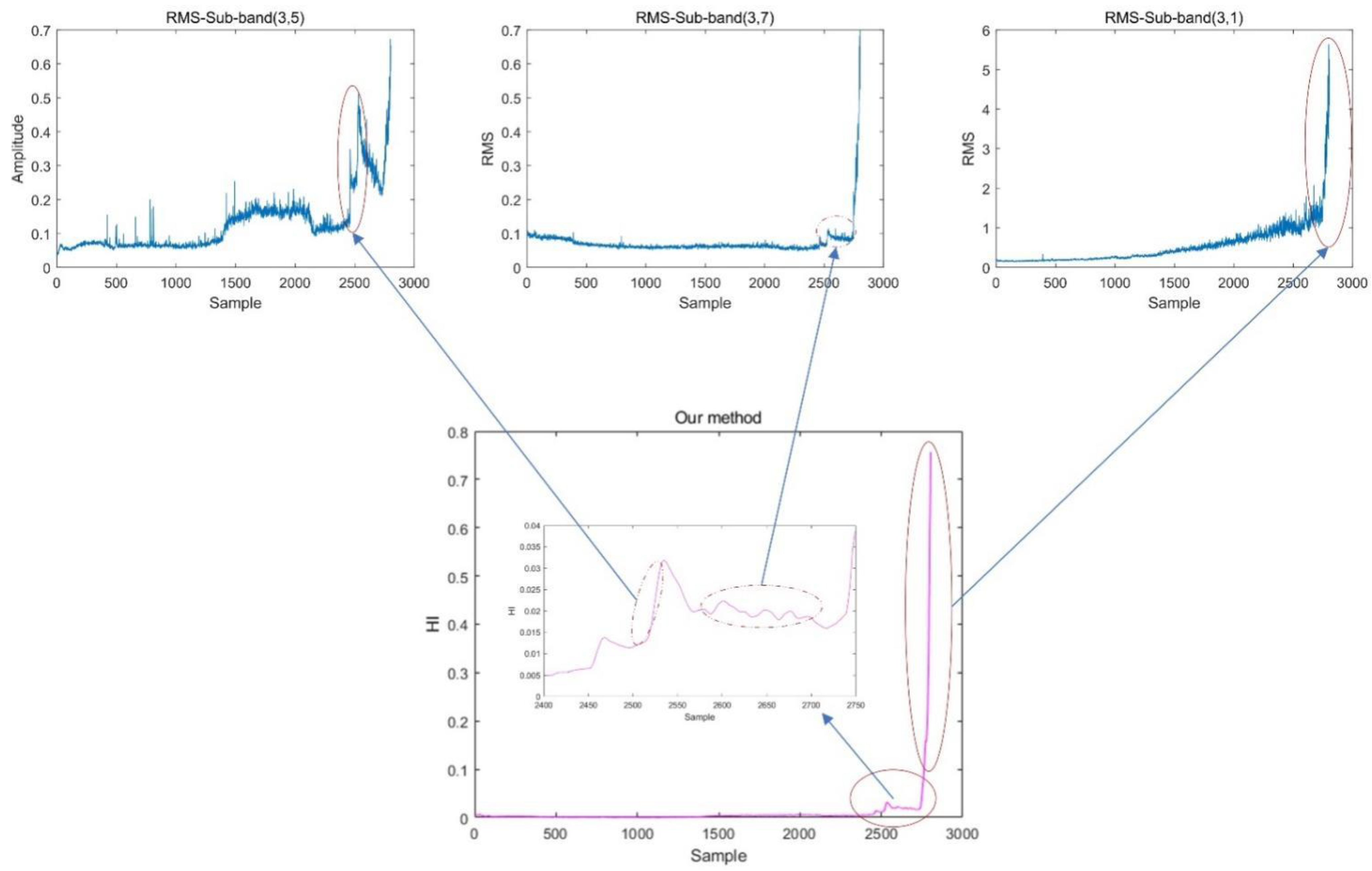
• Discrete wavelet packet transform (DWPT) and principal component analysis (KPCA) were combined to construct new health indicators to solve the labeling problem of RUL prediction. Compared to the life-percentage-style linear HI, this HI can better reflect the bearing degradation trend and retain the time–frequency characteristics of the signal, which is beneficial to the learning of the prediction model.
• A convolutional bidirectional long- and short-term memory neural network (CNN-BiLSTM) was designed for RUL prediction. Convolution can extract signal features from different scales, and combined with the BiLSTM network, the model can take into account both temporal and spatial features of the signal to improve prediction accuracy.
• Experimental data based on rolling bearing dataset were used to verify the effectiveness of the method.

The remainder of this paper is organized as follows. Section 2 provides the theoretical background. Section 3 introduces the method proposed in this paper. Section 4 describes the experimental procedure and the analysis of the results in detail. Section 5 concludes the paper.

2. Theoretical Background

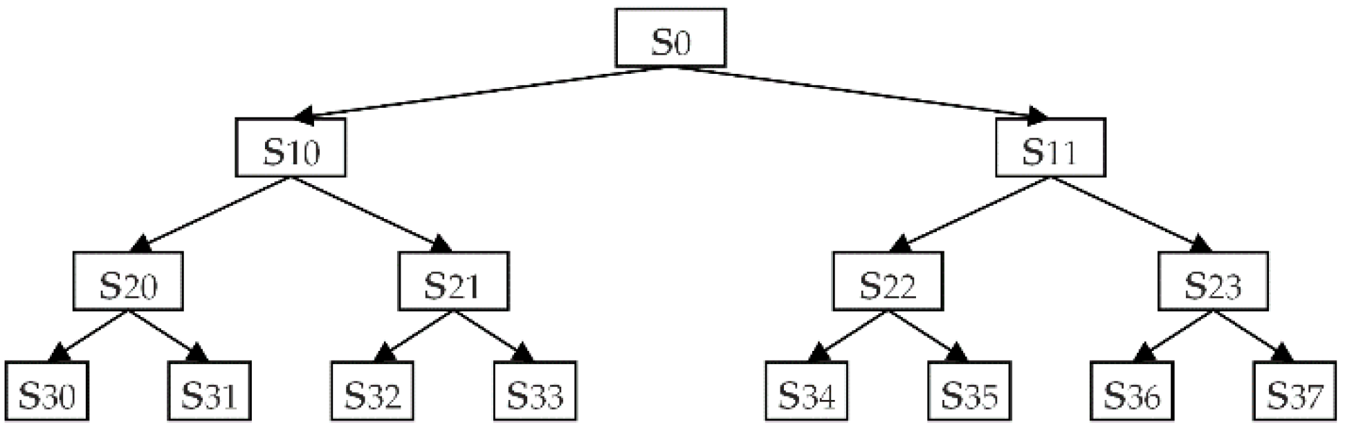
2.1. Discrete Wavelet Packet Transform (DWPT)

The discrete wavelet transform can describe the local characteristics of vibration signals in the time and frequency domains and is a very effective signal analysis method, which is often used for signal preprocessing for bearing fault diagnosis and life prediction [26].

In this study, the bearing vibration signal was preprocessed based on DWPT in order to construct HI. The algorithms for wavelet packet decomposition and reconstruction are shown in Equations (1) and (2), respectively.

$$\{\begin{array}{c}{d}_i^{j,2n}={\displaystyle \sum _k{p}_{k-2l}{d}_k^{j-1,n}}\\ d_l^{j,2n+1}={\displaystyle \sum _k{q}_{k-2l}{d}_k^{j-1,n}}\end{array}$$

(1)

$$d_l^{j-1,n}={\displaystyle \sum _k{p}_{l-2k}{d}_k^{j,2n}+{\displaystyle \sum _k{q}_{l-2k}{d}_k^{j,2n+1}}}$$

(2)

where p and q are filter coefficients; d is the wavelet packet decomposition coefficient; k and l are the number of decomposition layers; and j and n are wavelet packet node numbers.

Figure 1 is a schematic diagram of the three-layer wavelet packet decomposition structure, where S0 is the original signal, S10 is the low-frequency part of the original signal, S11 is the high-frequency part of the original signal, and so on. As can be seen from the figure, the wavelet packet transform can decompose both the low- and high-frequency parts of the signal uniformly and has higher time–frequency resolution than the wavelet transform, making it more effective in analyzing nonsmooth signals (e.g., bearing vibration signals) [20]. In this study, the db4 mother wavelet was used to decompose the original vibration signal into three levels of wavelet packets to obtain eight sub-bands.

2.2. Kernel Principal Component Analysis (KPCA)

Kernel principal component analysis (KPCA) [27] is a nonlinear feature extraction method that is often used for feature extraction and fusion of bearing signals [28]. The kernel function was first introduced to map the original data space to a high-dimensional feature space, and PCA was then performed to reduce the dimensionality of the analysis. The quality of the nonlinear features thus extracted was much better.

Let the data set with M samples be $\left\{x_1,x_2, \cdots ,x_i\right\}(i=1,2, \dots ,M)$, $x_i\in R^N$ and the sample dimension be N. Normalize the high-dimensional spatial data so that it satisfies the following:

$$\frac{1}{M}{\displaystyle \sum _{i=1}^M\phi (x_i)}=0$$

(3)

where $\phi$ is a nonlinear mapping function that enables the mapping of the low-dimensional spatial feature $x_i$ to the higher dimensional space $F:\phi (x_i)$.

The covariance matrix of $F$ space is expressed as follows:

$$C=\frac{1}{M}{\displaystyle \sum _{i=1}^M\phi (x_i)}\phi {(x_i)}^T$$

(4)

The eigenvalues of the covariance matrix are $\lambda$, and the eigenvectors are $v$, both of which satisfy the following:

$$Cv=\lambda v$$

(5)

After transforming each sample into $\phi (x_k)$, make inner product with Equation (5):

$$\phi (x_k)Cv=\lambda \phi (x_k)v$$

(6)

The linear representation of the feature vector is as follows:

$$v={\displaystyle \sum _{i=1}^M{\alpha }_i\phi (x_i)}$$

(7)

Simultaneous Formulas (4)–(7) can be obtained:

$$\frac{1}{M}{\displaystyle \sum _{i=1}^M{\alpha }_i{\displaystyle \sum _{j=1}^M\left[\phi (x_k)\phi (x_j)\right]}}\left[\phi (x_j)\phi (x_i)\right]=\lambda {\displaystyle \sum _{i=1}^M{\alpha }_i\left[\phi (x_k)\phi (x_i)\right]}$$

(8)

Nonlinear mapping from input space to high-dimensional feature space can be realized by kernel function inner product operation. The kernel function selected in this study is a Gaussian radial basis function, whose expression is as follows:

$$k(x_i,x_j)=\exp (-\gamma {\Vert x_i-x_j\Vert }^2)$$

(9)

where parameter $\gamma$ is used to control the range of action of the kernel function.

Define the $M\times M$ dimensional matrix K, where the elements can be represented using the following kernel function:

$$K=\left[\begin{array}{ccc}k(x_1,x_1)& \cdots & k(x_1,x_m)\\ ⋮& \ddots & ⋮\\ k(x_m,x_1)& \cdots & k(x_m,x_m)\end{array}\right]$$

(10)

The kernel matrix is used to represent Equation (8), which can be simplified as follows: $K\alpha =M\lambda \alpha$. The eigenvalues and eigenvectors of the kernel matrix can be derived from the simplified Equation (8), which in turn leads to the normalized eigenvector $v^k(k=1,2, \dots ,M)$ of the covariance matrix. Then, the k-th linear principal element of the sample $x$ can be obtained as follows:

$$h_k=v^k\phi (x)={\displaystyle \sum _{i=1}^M{\alpha }_i^{k}K(x_i,x)}$$

(11)

The cumulative contribution of features is calculated and the principal element is selected as follows:

$${\displaystyle \sum _{k=1}^p{\lambda }_k/}{\displaystyle \sum _{i=1}^m{\lambda }_i\ge 0.90}$$

(12)

where ${\lambda }_1\ge {\lambda }_2\ge {\lambda }_3\dots \ge {\lambda }_m$ is the eigenvalue of the kernel matrix.

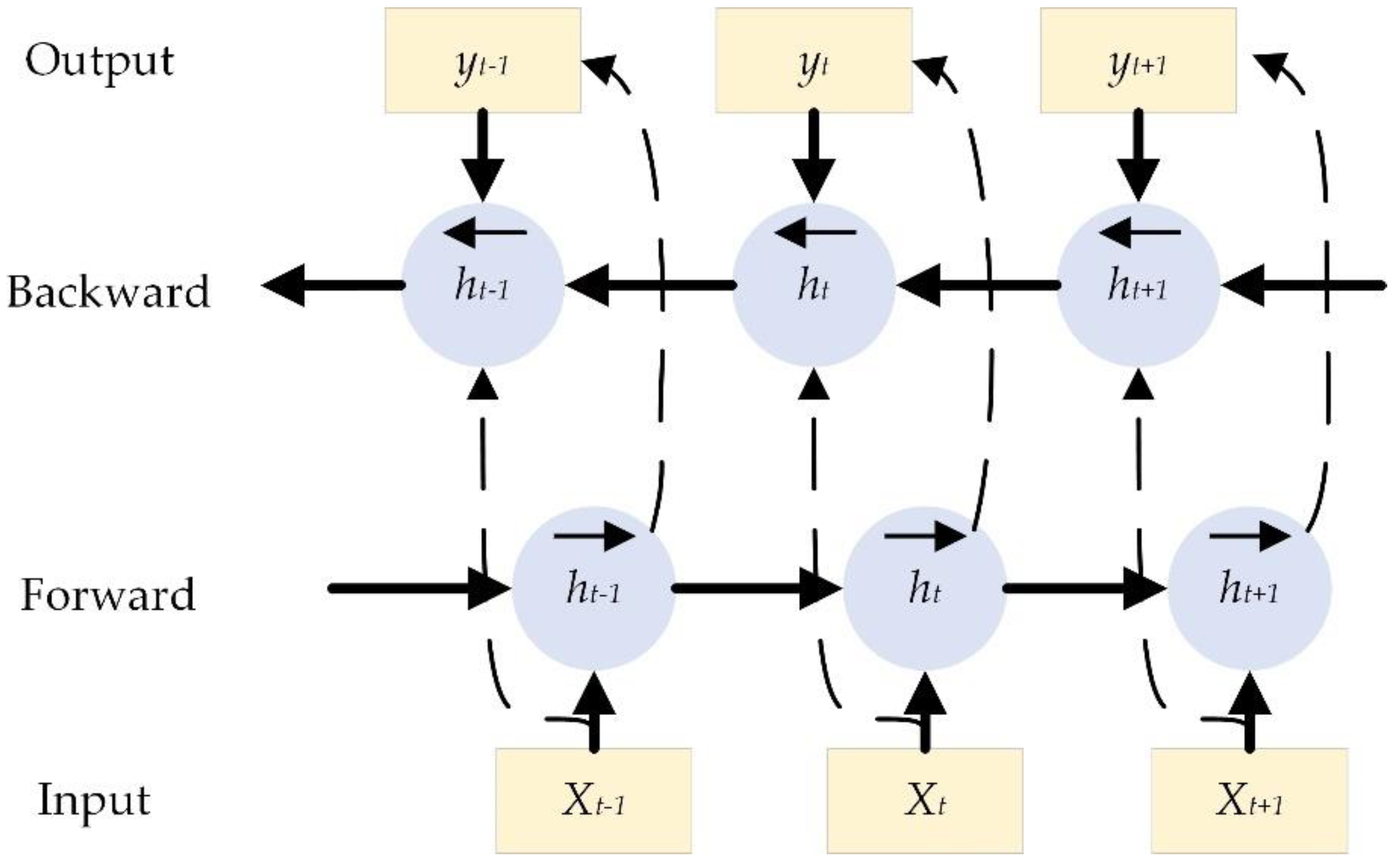
2.3. Bidirectional Long Short-Term Memory Neural Network (BiLSTM)

Long short-term memory neural network (LSTM) [29] is an improvement on the recurrent neural network (RNN). It solves the RNN gradient disappearance and gradient explosion problems by introducing forgetting gates and can efficiently learn the nonlinear features of time series.

As a deep learning neural network model, each neuron of LSTM is a memory cell with three gates, which are forgetting gate $f_t$, input gate $i_t$, and output gate $o_t$. The whole update process is shown in Equations (13)–(18).

The forgetting gate $f_t$ determines what information is discarded and is determined by both the current input and the output of the previous sequence.

$$f_t=\sigma \left(W_f·\left(h_{t-1},x_t\right)+b_f\right)$$

(13)

where $\sigma$ is the sigmoid activation function; $W_f$ is the weight vector; $b_f$ is the base vector; and $C_{t-1}$ denotes the cell state, which is used to store the memory information of the previous moment.

Update gate $i_t$ determines what information is stored and updates the cell state as follows:

$$i_t=\sigma (W_i·\left(h_{t-1},x_t\right)+b_c$$

(14)

$${\tilde{C}}_t=tanh(W_c·\left(h_{t-1},x_t\right)+b_c$$

(15)

$$C_t=f_t·C_{t-1}+i_t·{\tilde{C}}_t$$

(16)

where $tanh$ is the activation function, ${\tilde{C}}_t$ is the candidate vector for the current new state information; $f_t·C_{t-1}$ denotes the information to be forgotten; $i_t·{\tilde{C}}_t$ is the information to be retained; and $C_t$ is the current cell state.

$$o_t=\sigma \left(W_o·\left(h_{t-1},x_t\right)+b_o\right)$$

(17)

$$h_t=o_t·tanh\left(C_t\right)$$

(18)

where $o_t$ represents the output of information from the output gate, and $h_t$ is the output of the memory cell, which will also be input in the next LSTM cell.

The BiLSTM [30,31] consists of two LSTMs that pass information from the forward and reverse directions, respectively, compared to the LSTM and can associate both past and future states. The Bi-LSTM structure is shown in Figure 2, and its output is as follows [32].

$$h_t=[\overrightarrow{h_t},\overleftarrow{h_t]}$$

(19)

where $\overrightarrow{h_t}$ is the result of forward propagation, and $\overleftarrow{h_t}$ is the result of backward propagation.

2.4. Convolutional Neural Network (CNN)

Convolutional neural networks [33] have the characteristics of local connectivity and weight sharing. One-dimensional convolutional neural networks can perform feature extraction on time-domain signals and are commonly used in the field of bearing fault diagnosis [34].

Convolutional neural networks usually consist of three types of network layers: convolutional layer, pooling layer, and fully connected layer. The convolutional layer can implement convolutional operations for feature extraction, the pooling layer can reduce the feature dimensionality and prevent overfitting, and the fully connected layer can perform nonlinear combination of the extracted features.

The formula for one-dimensional convolution is as follows:

$$Z^{l+1}=\left[Z^l\ast w^{l+1}\right]+b={\displaystyle \sum _{x=1}^f\left[Z_k^l(s_0+x)w_k^{l+1}(x)\right]}+b$$

(20)

The maximum pooling equation is as follows:

$$A_i^{l+1}(j)=\underset{(j-1)W+1\le jW}{\max }\left\{F_i^l(t)\right\}$$

(21)

where $Z^l$ is the convolutional input of layer l + 1, and $Z^{l+1}$ is the output of layer l + 1; b is the amount of variance; $w_k^{l+1}$ is the weight of layer l + 1; f is the convolutional kernel size; s₀ is the convolutional step size; $F_i^l(t)$ is the value of the t-th neuron in the i-th feature of layer l; W is the pooling region; and $A_i^{l+1}$ is the output of the neuron of layer l + 1.

3. The Proposed Framework

The overall block diagram of the proposed method is shown in Figure 3. Firstly, the original vibration signal was subjected to discrete wavelet packet transform (DWPT) to obtain eight sub-bands and extract the RMS values of different sub-bands. Then, KPCA was used to downscale the multidimensional RMS to obtain HI. Finally, the remaining lifetime prediction was performed by CNN-BiLSTM network.

(1)

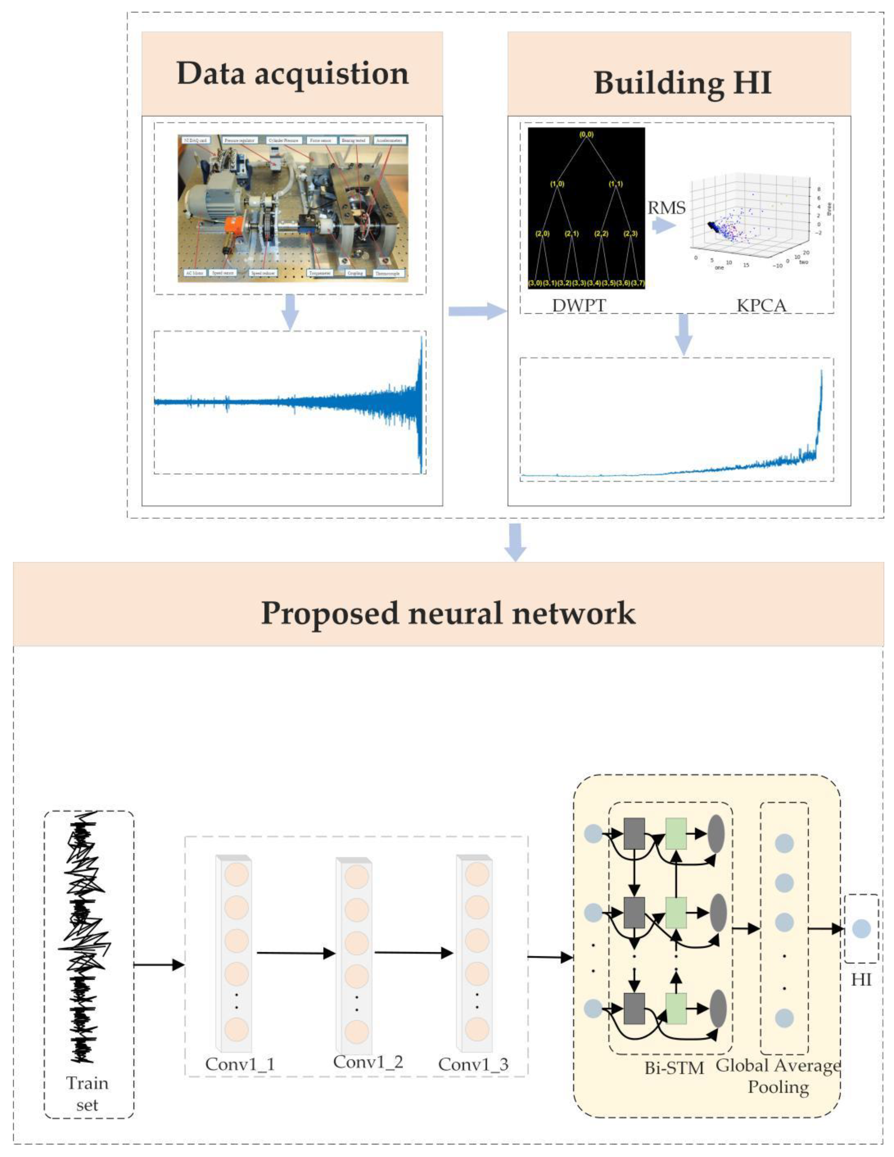
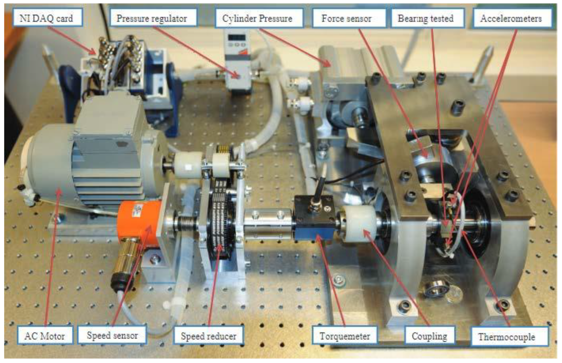
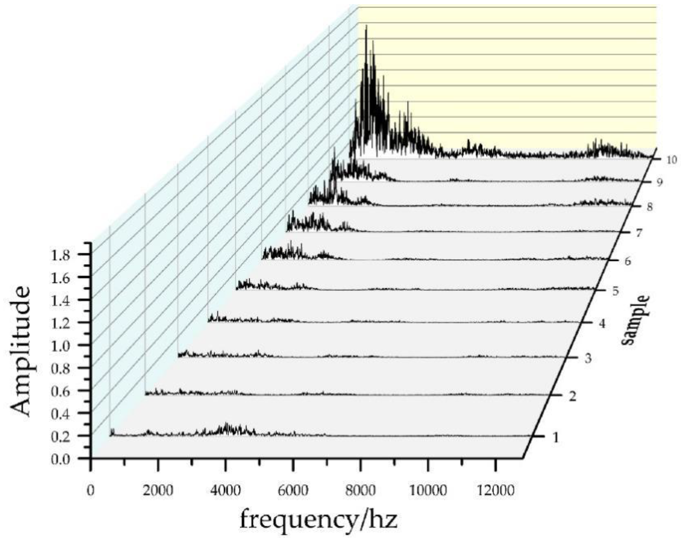
Data acquisition: The accelerometers were placed on the horizontal and vertical axes with sampling frequency of 25.6 KHZ, sampling interval of 10 s, and sampling time of 0.1 s. Sampling was performed under three working conditions.

(2)

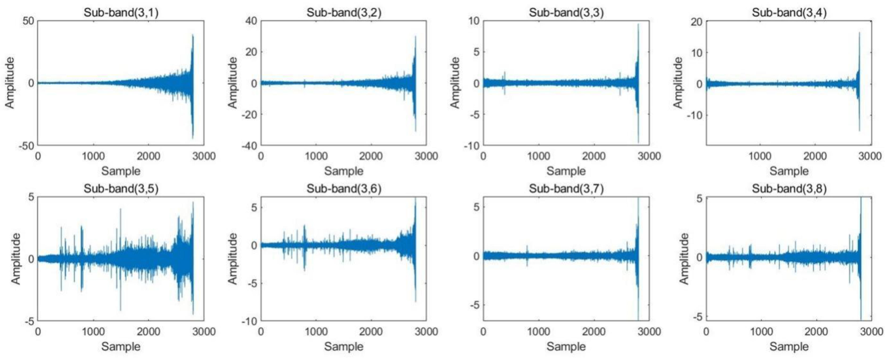
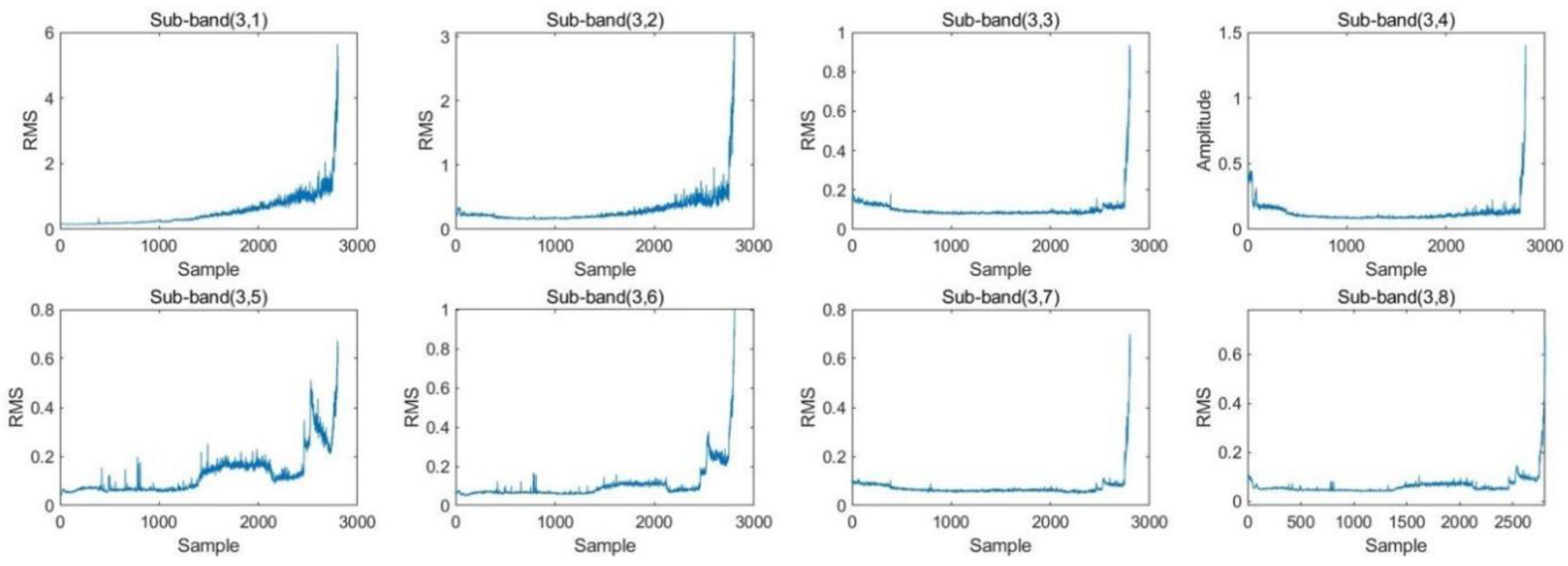
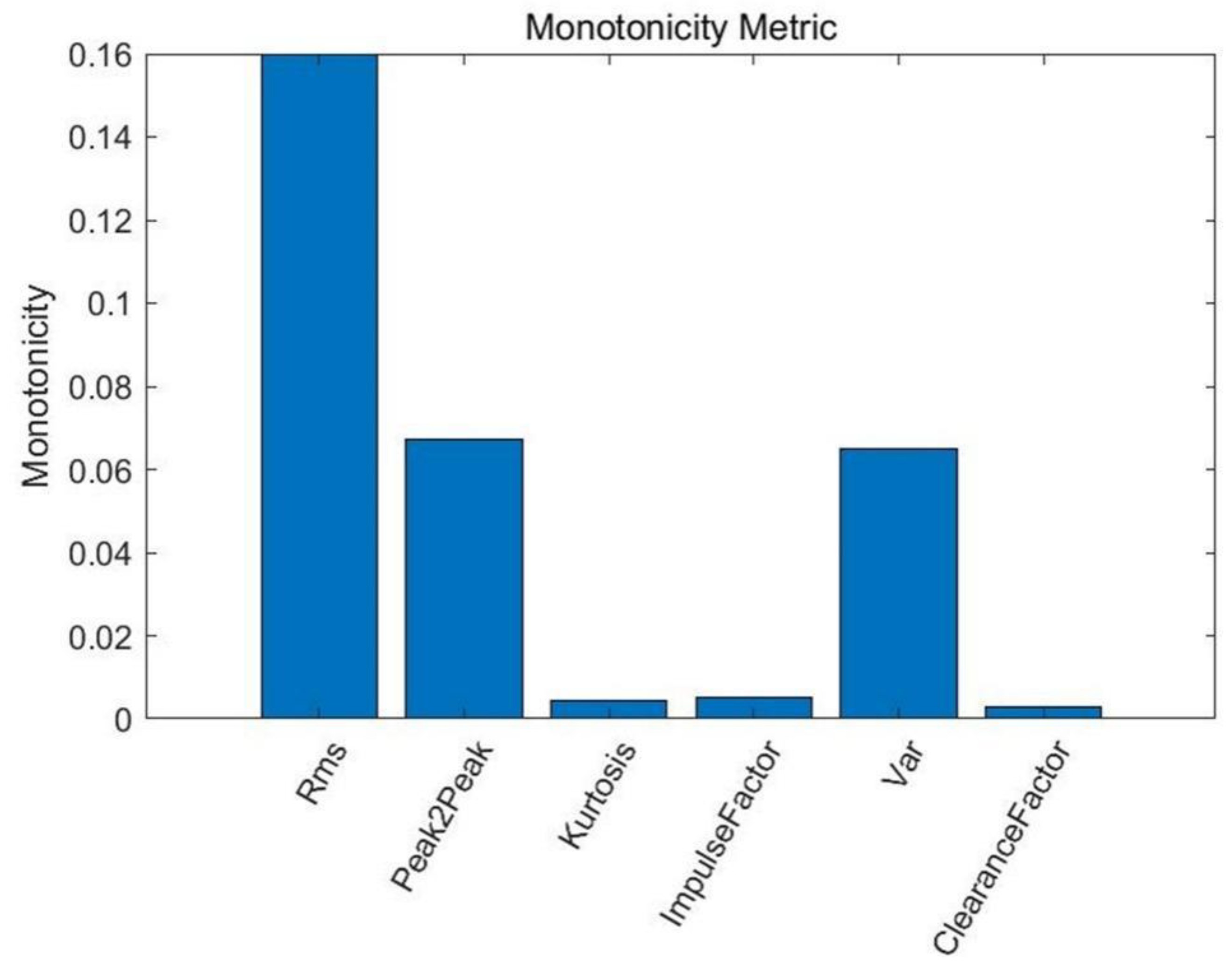
Building health indicators: The original vibration signal was decomposed into eight sub-bands using DWPT. The sub-bands were reconstructed according to the coefficients, and RMS values were extracted. The multidimensional RMS values were dimensionalized using the KPCA algorithm, and low-dimensional sensitive features were selected as HI and used as training labels for the prediction network.

(3)

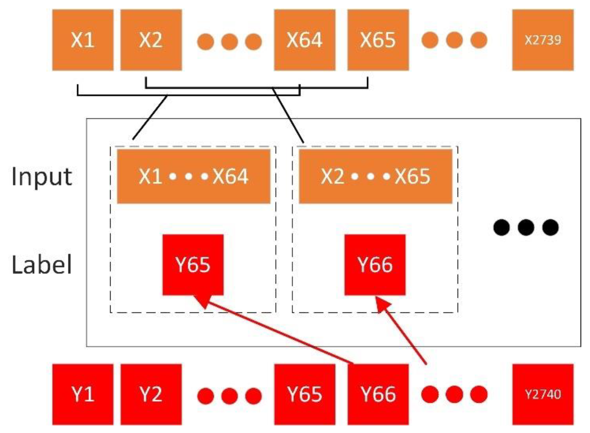
Proposed neural network: The spatial features of the signal were extracted using a convolutional network followed by a BiLSTM layer to extract temporal features from the forward and reverse directions. The global average pooling layer in the model can pay attention to the overall information, which is conducive to model prediction [35]. The mean square error was used as the loss function, and the optimizer was Adam. The input to the network was RMS at the current moment, and the output was the HI at the future moment.

4. Experiments and Results

4.1. Data Description

To verify the effectiveness of the proposed method, the PHM 2012 Challenge dataset was used in this study. The data was collected and obtained from the PRONOSTIA testbed, as shown in Figure 4.

The acquisition device was used for 17 full-life cycle experiments of the bearing under three operating conditions, and a total of 17 sets of data were collected in the horizontal and vertical directions of the bearing using an accelerometer. The sampling frequency of the accelerometer sensor was 25.6 kHZ, and the experimental setup recorded the vibration signals at 10 s intervals with a sampling time of 0.1 s [36]. Under working condition I, bearings 1-1 to 1-7 were tested with motor speed of 1800 rpm and load of 4000 N. Under working condition II, bearings 2-1 to 2-7 were tested with motor speed of 1650 rpm and load of 4200 N. Under working condition III, bearings 3-1 to 3-3 were tested with motor speed of 1500 rpm and load of 5000 N. Details of the data are shown in

Table 1. Operating condition of the PHM2012 dataset.

Working Condition	Load(N)	Rotation Speed	Dataset
1	4000	1800 rpm	Bearing 1-1 (train)
			Bearing 1-2 (train)
			Bearing 1-3 (test)
			Bearing 1-4 (test)
			Bearing 1-5 (test)
			Bearing 1-6 (test)
			Bearing 1-7 (test)
2	4200	1650 rpm	Bearing 2-1 (train)
			Bearing 2-2 (train)
			Bearing 2-3 (test)
			Bearing 2-4 (test)
			Bearing 2-5 (test)
			Bearing 2-6 (test)
			Bearing 2-7 (test)
3	5000	1500 rpm	Bearing 3-1 (train)
			Bearing 3-2 (train)
			Bearing 3-3 (test)

.

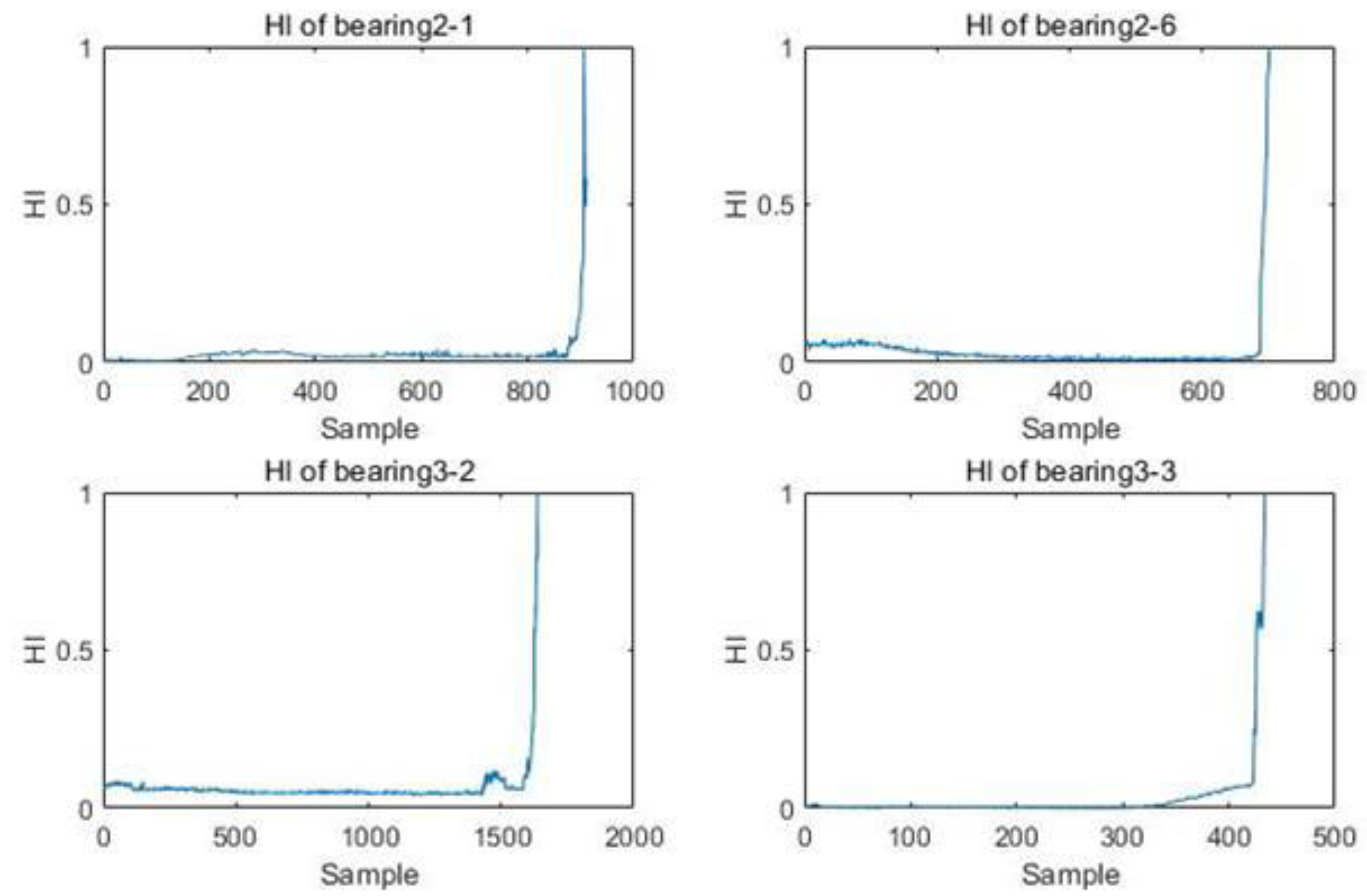
4.2. Construction of Health Indicators

In this section, we describe the process of HI construction in detail. Figure 5 shows the original vibration signal of bearing 1-1. As can be seen, the vibration signal amplitude of bearing 1-1 initially fluctuated roughly smoothly. The vibration signal showed a gradual upward trend with increase in time and increased sharply at the later stage.

In the original time-domain signal shown in Figure 5, every 2560 consecutive points constitute a sample. These samples were processed by fast Fourier transform to obtain the corresponding frequency-domain samples. In Figure 6, 10 frequency-domain samples are shown. In the figure, the time corresponding to these samples increases with the sample number. For example, sample 1 corresponds to the beginning of the bearing life cycle, and sample 10 corresponds to the end of the bearing life cycle.

As can be seen from Figure 6, the bearings had different degrees of amplitude increase in different frequency sections. The low-frequency vibration was due to rotation frequency, rolling body, and internal and external fault frequency of rolling. The high-frequency vibration was caused by the inherent frequency of each component of the bearing. When the bearing failed, the shape and quality of the component changed, affecting the high-frequency vibration.

To construct the HI, the original vibration signal was first decomposed into wavelet packets using db4 wavelets for three-level decomposition [20]. Reconstruction was performed according to the reconstruction coefficients to obtain eight sub-bands. The reconstructed sub-bands are shown in Figure 7. It can be seen that the eight sub-bands exhibited different trends, and each contained degradation characteristics of different frequency bands.

The RMS was extracted for each of the eight sub-bands, and the RMS values for each sub-band were obtained, as shown in Figure 8.

As can be seen from Figure 8, the RMS extracted from the eight sub-bands had different trends. During the whole life cycle of the bearing, the RMS of some sub-bands showed an increasing trend, while the RMS of other sub-bands showed significant fluctuations. The RMS of all sub-bands showed a steep upward trend in the last part of the life cycle, while the RMS of some sub-bands showed sensitivity at the beginning of the wear. This indicates that different sub-bands carry different degradation information.

In order to fuse the most important degradation information exhibited by all sub-bands, the RMS of the eight sub-bands were feature fused using the KPCA algorithm. First, the eight sub-band RMS sequences shown in Figure 8 were selected to construct an eight-dimensional high-dimensional feature set. Then, the KPCA algorithm was used to reduce the dimensionality of the feature set. Finally, the first principal element (contribution rate >90%) was selected as the final HI.

Table 2. Contribution rate of partial principal components.

Principal Component Serial Number	Contribution Rate	Cumulative Contribution Rate
1	0.919	0.919
2	0.061	0.980
3	0.019	0.999

shows the contribution rates of the principal elements. The final construction results are shown in Figure 9.

Figure 9 shows a comparison of the values of RMS extracted from the sub-bands and RMS extracted using the method proposed in this study. The sub-band RMS fluctuated a lot, and the curves were messy. The method proposed in this paper could fuse the important characteristics of each sub-band, such as the sudden increase in RMS of sub-band (3,5) near sample 2500, which reflected the sensitivity at the early stage of wear; the gentle fluctuation of RMS of sub-band (3,7) at sample 2600 and the decrease in HI, which reflected the sensitivity at the recovery period of wear; and the sharp increase in RMS of sub-band (3,1) at the last part of the life cycle, which reflected the sensitivity of the late wear period. The proposed HI thus contained more comprehensive information on bearing degradation and the curve was smoother, reflecting its superiority as an HI. To further illustrate the superiority of the proposed HI, the HI of bearings 2-1, 2-6, 3-2, and 3-3 under different operating conditions were extracted, and the results are shown in Figure 10.

The health factor, which reflects the degradation trend of the bearing, needs to have a strong correlation with the degradation trend of the bearing. The physical degradation process of the bearing is irreversible, so the health factor should also have a similar monotonic change trend [37]. Monotonicity indexes are widely used in the evaluation of health factor performance. Yang et al. [38] obtained the optimal HI by optimizing the monotonicity index of HI. Lin et al. [39] used ensemble stacked autoencoders to construct health factors for bearings and evaluated their performance using monotonicity metrics.

We compared the performance of the proposed HI with the original RMS using the metric of monotonicity according to the following equation:

$$Mon(X)=\frac{1}{K-1}\left|No.ofd/d_x>0-No.ofd/d_x<0\right|$$

(22)

where X denotes the feature sequence; K denotes the total number of features; and $No.ofd/d_x>0$ and $No.ofd/d_x<0$ denote the number of positive and negative variances, respectively. The higher the Mon score, the better the monotonicity and the better the index performance. The results are shown in

Table 3. HI performance analysis using monotonicity.

Bearing	Monotonicity of RMS	Monotonicity of Proposed HI
1-1	0.161	0.961
1-2	0.102	0.962
1-3	0.047	0.936
1-4	0.051	0.917
1-5	0.101	0.959
1-6	0.099	0.908
1-7	0.149	0.933
2-1	0.087	0.915
2-2-	0.132	0.941
2-3	0.141	0.907
2-4	0.097	0.913
2-5	0.089	0.968
2-6	0.127	0.947
2-7	0.152	0.903
3-1	0.074	0.931
3-2	0.046	0.903
3-3	0.047	0.933

.

From the table, we can see that the proposed HI had better monotonicity, which proves the superiority of the proposed method.

4.3. RUL Prediction

In this section, we outline the development of a CNN-BiLSTM prediction model with RMS input and HI labels and discuss the effect of model parameters on prediction accuracy. Bearing 1-1 was used as an example to develop a detailed description.

4.3.1. Input Selection

It is convenient to process raw vibration signals of bearings in the time domain, and features such as Rms, Peak2Peak, Kurtosis, Impulse Factor, Var, and Clearance Factor are commonly used in the analysis of the remaining service life of bearings and as inputs to prediction networks [4,40].

We can extract many features, such as time domain and frequency domain, from vibration signals. These features have different representation abilities for vibration signals. Some features are not helpful or even cause interference for characterizing signals. Therefore, it is very important to select appropriate features [41]. The degradation process is an accumulation of random fatigue failure processes, so it should have a certain overall increasing or decreasing trend on the time axis, i.e., the characteristic quantity should have certain monotonicity [37]. Zhang et al. [42] extracted signal time-domain, frequency-domain, and time–frequency-domain correlation features and defined metrics such as monotonicity for feature selection based on the trend and residuals of the features. Tian et al. extracted 10 features of bearing vibration signals and used the monotonicity index to screen good features as input to the neural network [43].

Different time-domain features have different characterization capabilities for the original signal, and monotonicity continues to be used to assess the characterization capabilities of time-domain features.

The monotonicity score was calculated for the time-domain features, and the results are shown in Figure 11.

As can be seen from Figure 11, the Rms monotonicity of the original vibration signal was the best, and Rms was chosen here as input to the prediction network.

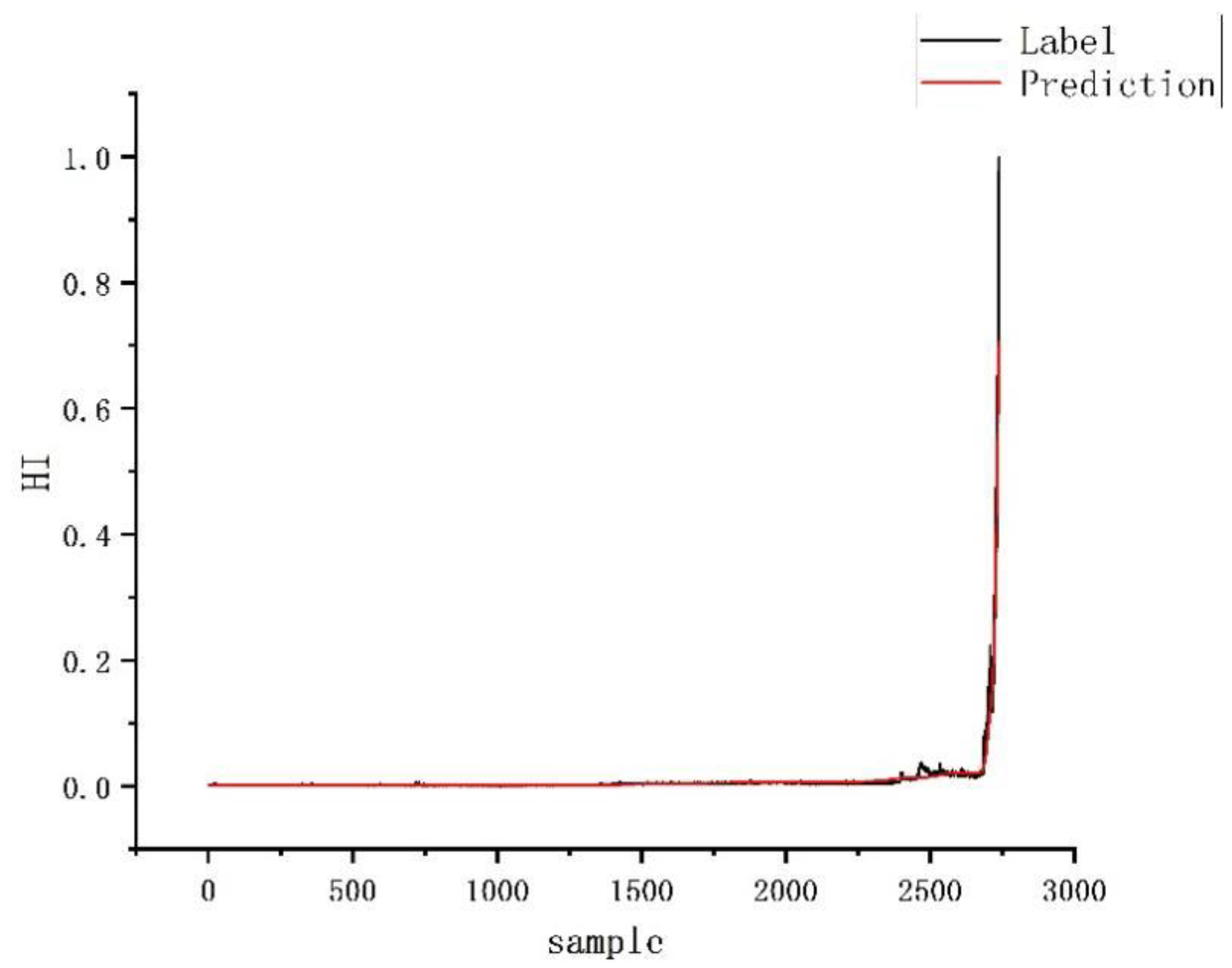
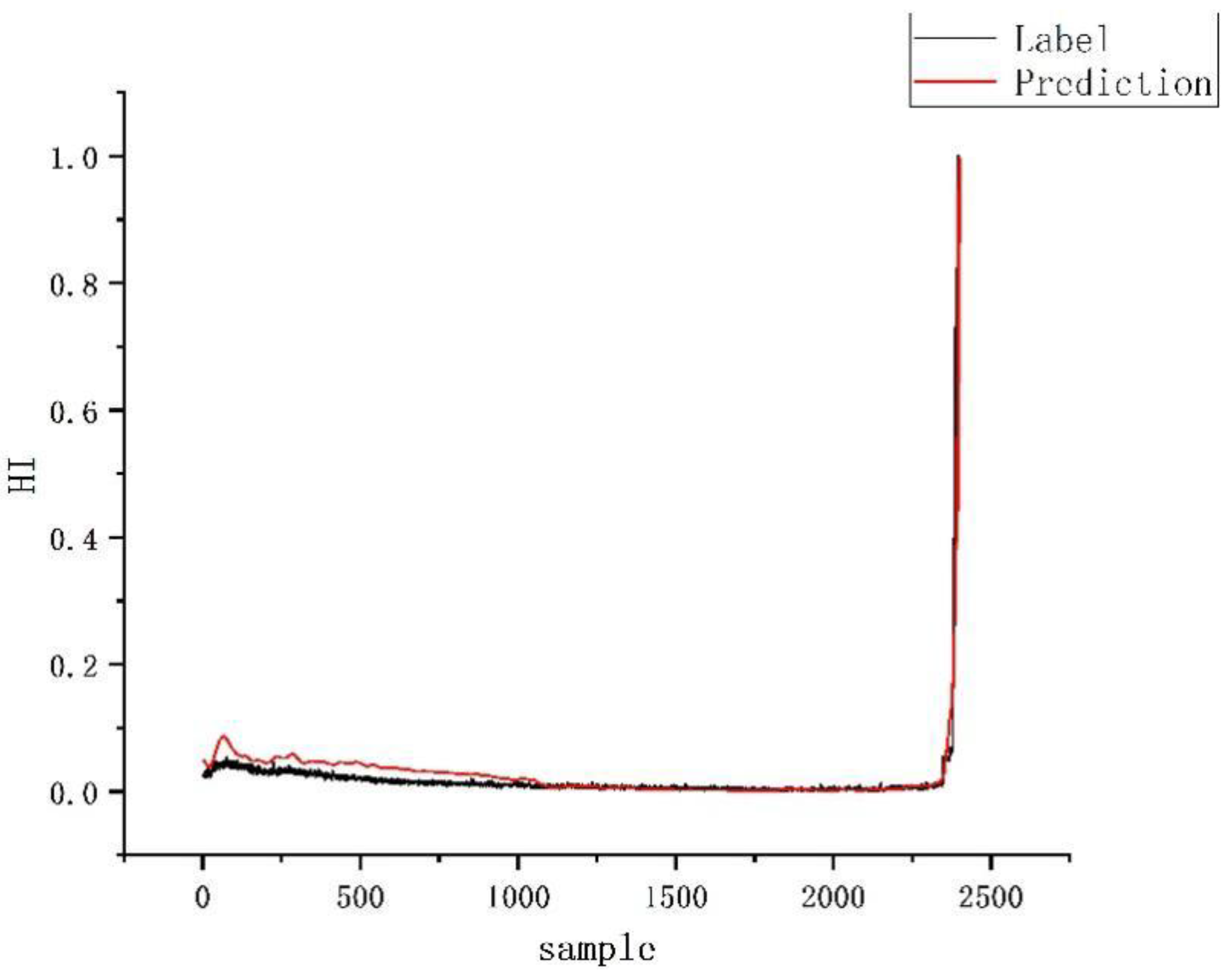
4.3.2. Training and Test of CNN-BiLSTM Model

Before training and testing a prediction model, it is necessary to construct the dataset and determine the correspondence between the input Rms and output HI labels. Suppose the Rms sequence is $\left[X_1,X_2,X_3,X_4\right]$ and the HI sequence is $\left[Y_1,Y_2,Y_3,Y_4\right]$, then the prediction relationship of the network is $F(\left[X_1,X_2\right])=Y_3$, $F(\left[X_2,X_3\right])=Y_4$. A sliding window was used to take the value of the Rms sequence with a window width of 64 and a sliding step of 1. The specific correspondence is shown in Figure 12. The final sample format (number of samples, time step, and dimension) obtained was (2739, 64, and 1).

For the CNN-BiLSTM model, Adam optimizer with an initial learning rate of 0.001 was used, and in order to maximize the optimization of the network parameters, a decreasing learning strategy was used to reduce the learning rate by 10⁻⁶ per round. The training results of the model are shown in Figure 13, and the prediction results of the training set were almost identical to the real HI labels.

Signal processing was performed as described in the previous section for HI construction, and finally the trained CNN-BiLSTM model was used for prediction of bearing 1-5. The prediction results are shown in Figure 14. As can be seen, the prediction results are basically consistent with the real HI labels, which verifies the effectiveness of the method.

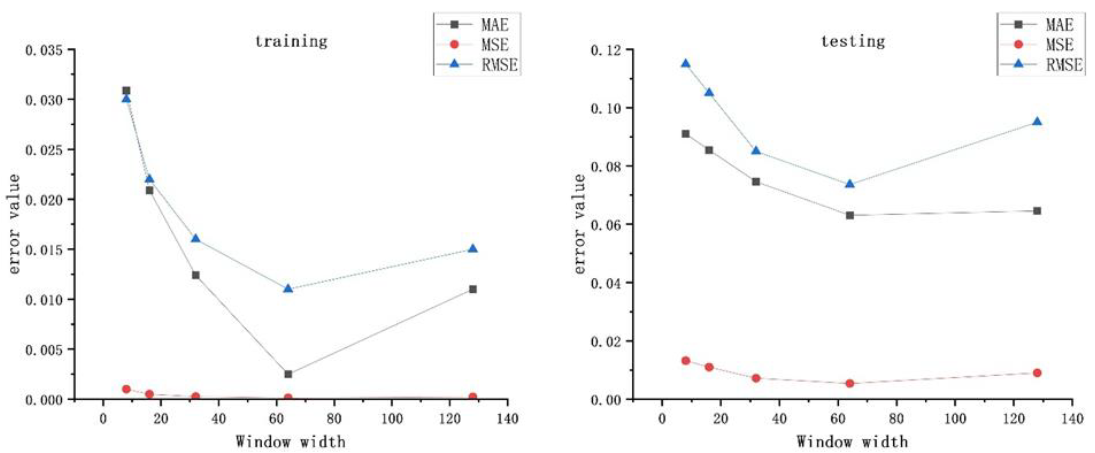
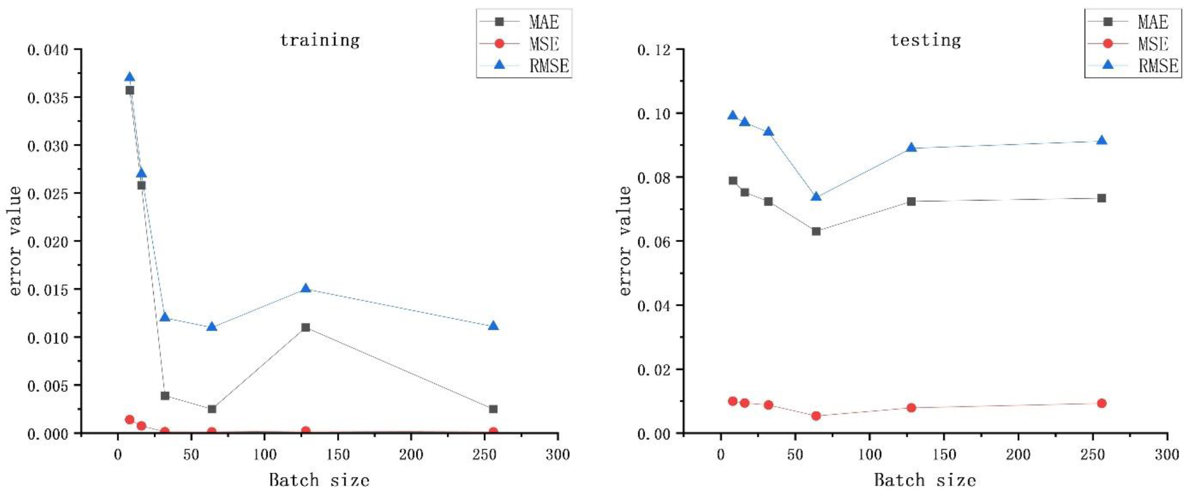
4.3.3. Selection of Hyper Parameters

In prediction models, the width of the sliding window and the size of the batch size are key hyperparameters that affect the performance of the model. This section discusses the effects of both parameters on the model performance.

The 2ⁿ facilitated the computer processor for optimization, and window widths of 8, 16, 32, 64, and 128 were used to shape the samples. The prediction model was then trained and tested. The models were evaluated using mean square error (MSE), root mean square error (RMSE), and mean absolute error (MAE). The errors on the training and test sets are shown in Figure 15.

The above metrics can be described as follows.

$$\mathrm{RMSE}=\sqrt{\frac{1}{N}{\displaystyle \sum _{i=1}^N{(y_i-{\widehat{y}}_i)}^2}}$$

(23)

$$\mathrm{MSE}=\frac{1}{N}{\displaystyle \sum _{i=1}^N{(y_i-{\widehat{y}}_i)}^2}$$

(24)

$$\mathrm{MAE}=\frac{1}{N}{\displaystyle \sum _{i=1}^N\left|y_i-{\widehat{y}}_i\right|}$$

(25)

where $y_i$ is the true label; ${\widehat{y}}_i$ is the predicted label; ${\overline{y}}_i$ is the mean of the actual labels; and N denotes the total number of samples.

As can be seen from Figure 15, on the training set, with the increase in the window width, each error showed a decreasing–increasing trend and the smallest error was at the window width of 64. On the test set, with the increase in the window width, the error showed irregular fluctuations and the smallest error was at the window width of 64. Therefore, the window width of 64 was chosen.

The batch size represents the number of data samples crawled in one training session. The batch size affects the training speed and model optimization. Batch sizes of 8, 16, 32, 64, 128, and 256 were selected, and the relationship between the three types of errors and batch size was observed. The results are shown in Figure 16.

From Figure 16, it can be seen that the three errors on the training set basically showed a decreasing trend with the increase of Batch size. However, in the test set, the three errors first decreased and then increased as the batch size increased. The errors increased significantly when the batch size exceeded 64, so 64 was chosen as the batch size.

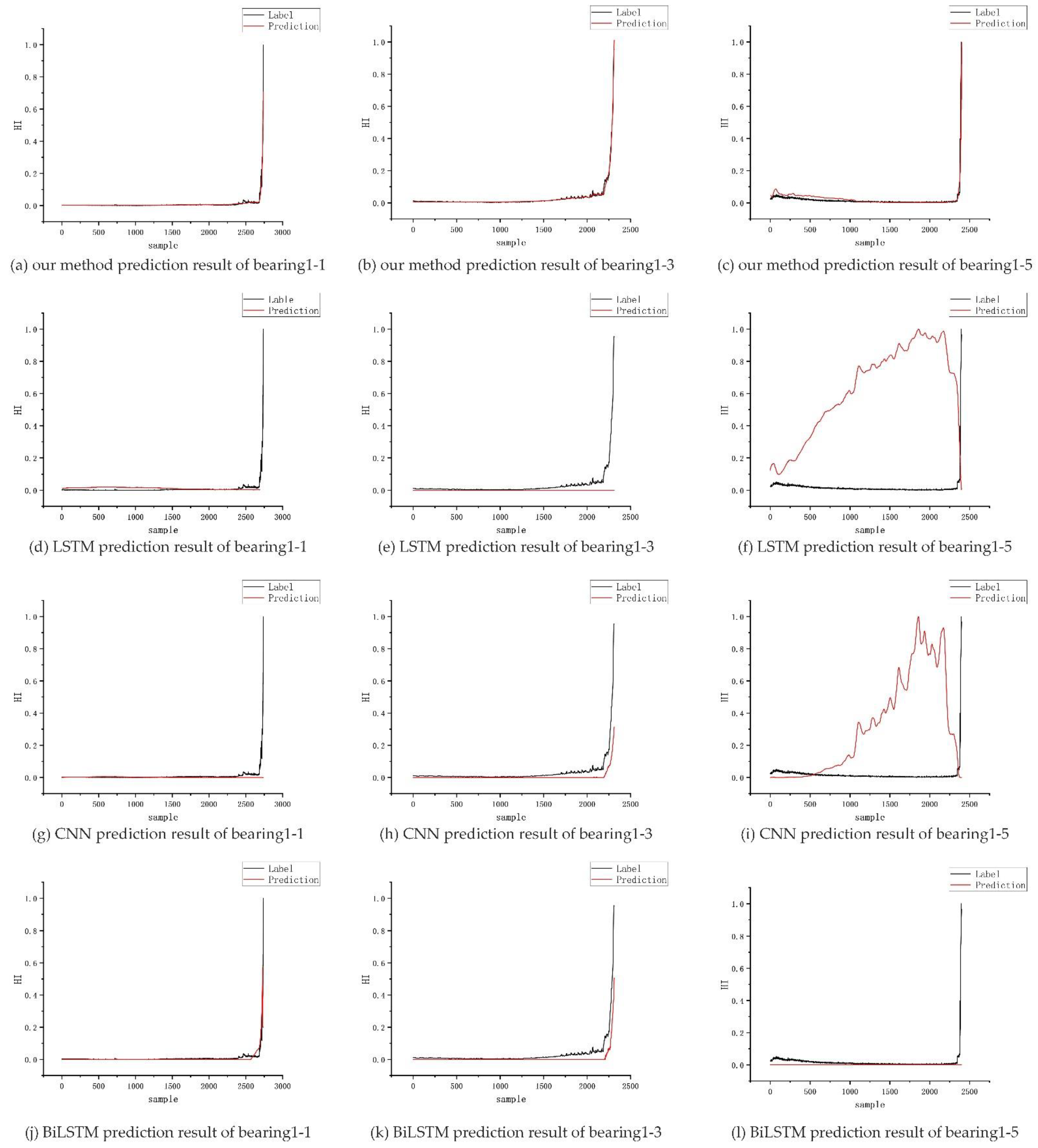
4.3.4. Results of Different Models

This section discusses the prediction effects of CNN, LSTM, and BiLSTM models on the PHM2012 dataset and compares them with the method proposed in this paper.

Prediction experiments were conducted on the dataset using each of the three models mentioned above, and the prediction results for bearings 1-1, 1-3, and 1-5 were visualized. The results are shown in Figure 17.

From Figure 17, it can be seen that the proposed method could accurately predict the degradation trend of the bearing, and the rest of the models had different degrees of problems. For example, both the LSTM and CNN models could not well predict the rapid degradation stage of bearing 1-1. The prediction effect of BiLSTM was better, but the fluctuation trend at the beginning of degradation could not be well predicted. Both the LSTM and CNN models could not well predict the rapid degradation stage of bearing 1-1. The prediction effect of BiLSTM was better, but the fluctuation trend at the beginning of degradation could not be well predicted. The BiLSTM model could not predict the rapid degradation trend of the bearing at the end of cycle 1-5. The CNN could roughly predict the degradation trend of the bearing from 1-3, but the accuracy was insufficient.

As shown in

Table 4. MSE for different prediction models.

Model (MSE)	Bearing 1-3	Bearing 1-4	Bearing 1-5	Bearing 1-6	Bearing 1-7	Bearing 2-3	Bearing 2-4	Bearing 2-5	Bearing 2-6	Bearing 2-7	Bearing 3-3
Proposed	0.0054	0.0031	0.007 6	0.0044	0.0048	0.0621	0.0091	0.0143	0.0087	0.1026	0.0078
CNN	0.1431	0.1101	0.1923	0.0942	0.2721	0.0623	0.0089	0.2641	0.3101	0.2176	0.1739
LSTM	0.2145	0.0671	0.2167	0.1743	0.0074	0.1473	0.1012	0.1149	0.2031	0.0098	0.2147
BiLSTM	0.0097	0.1431	0.1016	0.2497	0.1364	0.1824	0.2107	0.1087	0.1047	0.4102	0.3006

, the proposed model achieved the smallest prediction error on almost all bearings using MSE as an indicator, thereby showing the superiority of the proposed method.

5. Conclusions

The remaining service life prediction of bearings is a research focus. In this study, we established a suitable health indicator (HI) and proposed a prediction network combining CNN and BiLSTM. First, wavelet packet transform was performed on the original vibration signal of the bearing to obtain eight sub-bands, and the RMS of each of the eight sub-bands were extracted. The KPCA algorithm was then used to fuse the features of the extracted RMS of the eight sub-bands to obtain the HI of the bearing life cycle. The CNN-BiLSTM prediction network was then developed, which can extract the spatiotemporal features of the signal at the same time to improve prediction accuracy. The prediction network uses the RMS of the original signal at the current moment as the network input and the HI of the future moment as the network output. Experiments were conducted on the PHM2012 dataset to verify the effectiveness of the proposed prediction model.

References

1. Pech, M.; Vrchota, J.; Bednář, J. Predictive Maintenance and Intelligent Sensors in Smart Factory: Review. Sensors 2021, 21, 1470. [Google Scholar] [CrossRef] [PubMed]
2. Mao, W.; Liu, Y.; Ding, L.; Safian, A.; Liang, X. A New Structured Domain Adversarial Neural Network for Transfer Fault Diagnosis of Rolling Bearings Under Different Working Conditions. IEEE Trans. Instrum. Meas. 2021, 70, 3509013. [Google Scholar] [CrossRef]
3. Hamadache, M.; Jung, J.H.; Park, J.; Youn, B.D. A comprehensive review of artificial intelligence-based approaches for rolling element bearing PHM: Shallow and deep learning. JMST Adv. 2019, 1, 125–151. [Google Scholar] [CrossRef] [Green Version]
4. Cheng, H.; Kong, X.; Chen, G.; Wang, Q.; Wang, R. Transferable convolutional neural network based remaining useful life prediction of bearing under multiple failure behaviors. Measurement 2021, 168, 108286. [Google Scholar] [CrossRef]
5. Ma, S.; Zhang, X.; Yan, K.; Zhu, Y.; Hong, J. A Study on Bearing Dynamic Features under the Condition of Multiball–Cage Collision. Lubricants 2022, 10, 9. [Google Scholar] [CrossRef]
6. Qian, Y.; Yan, R.; Gao, R.X. A multi-time scale approach to remaining useful life prediction in rolling bearing. Mech. Syst. Signal Process. 2017, 83, 549–567. [Google Scholar] [CrossRef] [Green Version]
7. Xu, J.; Duan, S.; Chen, W.; Wang, D.; Fan, Y. SACGNet: A Remaining Useful Life Prediction of Bearing with Self-Attention Augmented Convolution GRU Network. Lubricants 2022, 10, 21. [Google Scholar] [CrossRef]
8. Bousdekis, A.; Magoutas, B.; Apostolou, D.; Mentzas, G. Review, analysis and synthesis of prognostic-based decision support methods for condition based maintenance. J. Intell. Manuf. 2018, 29, 1303–1316. [Google Scholar] [CrossRef]
9. El-Tawil, K.; Jaoude, A.A. Stochastic and nonlinear-based prognostic model. Syst. Sci. Control Eng. 2013, 1, 66–81. [Google Scholar] [CrossRef] [Green Version]
10. Rathore, M.S.; Harsha, S.P. Prognostics Analysis of Rolling Bearing Based on Bi-Directional LSTM and Attention Mechanism. J. Fail. Anal. Prev. 2022, 22, 704–723. [Google Scholar] [CrossRef]
11. Cerrada, M.; Sánchez, R.-V.; Li, C.; Pacheco, F.; Cabrera, D.; de Oliveira, J.V.; Vásquez, R.E. A review on data-driven fault severity assessment in rolling bearings. Mech. Syst. Signal Process. 2018, 99, 169–196. [Google Scholar] [CrossRef]
12. Mushtaq, S.; Islam, M.M.M.; Sohaib, M. Deep Learning Aided Data-Driven Fault Diagnosis of Rotatory Machine: A Comprehensive Review. Energies 2021, 14, 5150. [Google Scholar] [CrossRef]
13. Chen, D.; Qin, Y.; Wang, Y.; Zhou, J. Health indicator construction by quadratic function-based deep convolutional auto-encoder and its application into bearing RUL prediction. ISA Trans. 2021, 114, 44–56. [Google Scholar] [CrossRef] [PubMed]
14. Liu, Z.-H.; Meng, X.-D.; Wei, H.-L.; Chen, L.; Lu, B.-L.; Wang, Z.-H.; Chen, L. A Regularized LSTM Method for Predicting Remaining Useful Life of Rolling Bearings. Int. J. Autom. Comput. 2021, 18, 581–593. [Google Scholar] [CrossRef]
15. Nectoux, P.; Gouriveau, R.; Medjaher, K.; Ramasso, E.; Chebel-Morello, B.; Zerhouni, N.; Varnier, C. PRONOSTIA: An experimental platform for bearings accelerated degradation tests. In Proceedings of the IEEE International Conference on Prognostics and Health Management (PHM’12), Beijing, China, 23–25 May 2012. [Google Scholar]
16. Ning, Y.; Wang, G.; Yu, J.; Jiang, H. A Feature Selection Algorithm Based on Variable Correlation and Time Correlation for Predicting Remaining Useful Life of Equipment Using RNN. In Proceedings of the 2018 IEEE Condition Monitoring and Diagnosis (CMD), Perth, Australia, 23–26 September 2018. [Google Scholar]
17. Huang, G.; Li, H.; Ou, J.; Zhang, Y.; Zhang, M. A Reliable Prognosis Approach for Degradation Evaluation of Rolling Bearing Using MCLSTM. Sensors 2020, 20, 1864. [Google Scholar] [CrossRef] [Green Version]
18. Wang, X.; Mao, D.; Li, X. Bearing fault diagnosis based on vibro-acoustic data fusion and 1D-CNN network. Measurement 2021, 173, 108518. [Google Scholar] [CrossRef]
19. Zhang, X.; Cong, Y.; Yuan, Z.; Zhang, T.; Bai, X. Early Fault Detection Method of Rolling Bearing Based on MCNN and GRU Network with an Attention Mechanism. Shock Vib. 2021, 2021, 6660243. [Google Scholar] [CrossRef]
20. Duong, B.P.; Khan, S.A.; Shon, D.; Im, K.; Park, J.; Lim, D.-S.; Jang, B.; Kim, J.-M. A Reliable Health Indicator for Fault Prognosis of Bearings. Sensors 2018, 18, 3740. [Google Scholar] [CrossRef] [Green Version]
21. Zhang, N.; Wu, L.; Wang, Z.; Guan, Y. Bearing Remaining Useful Life Prediction Based on Naive Bayes and Weibull Distributions. Entropy 2018, 20, 944. [Google Scholar] [CrossRef] [Green Version]
22. Singleton, R.K.; Strangas, E.G.; Aviyente, S. Extended Kalman filtering for remaining-useful-life estimation of bearings. IEEE Trans. Ind. Electron. 2015, 62, 1781–1790. [Google Scholar] [CrossRef]
23. Zhang, Z.-X.; Si, X.-S.; Hu, C.-H. An Age- and State-Dependent Nonlinear Prognostic Model for Degrading Systems. IEEE Trans. Reliab. 2015, 64, 1214–1228. [Google Scholar] [CrossRef]
24. Hu, L.; Hu, N.-Q.; Fan, B.; Gu, F.-S.; Zhang, X.-Y. Modeling the Relationship between Vibration Features and Condition Parameters Using Relevance Vector Machines for Health Monitoring of Rolling Element Bearings under Varying Operation Conditions. Math. Probl. Eng. 2015, 2015, 123730. [Google Scholar] [CrossRef]
25. Song, L.; Wang, H.; Chen, P. Vibration-based intelligent fault diagnosis for roller bearings in low-speed rotating machinery. IEEE Trans. Instrum. Meas. 2018, 67, 1887–1899. [Google Scholar] [CrossRef]
26. Nguyen, H.N.; Kim, J.; Kim, J.M. Optimal sub-band analysis based on the envelope power Spectrum for effective fault detection in bearing under variable, low speeds. Sensors 2018, 18, 1389. [Google Scholar] [CrossRef] [Green Version]
27. Schölkopf, B.; Smola, A.; Mueller, K.-R. Nonlinear Component Analysis as a Kernel Eigenvalue Problem. Neural Comput. 1998, 10, 1299–1319. [Google Scholar] [CrossRef] [Green Version]
28. Shen, J.; Xu, F. Method of fault feature selection and fusion based on poll mode and optimized weighted KPCA for bearings. Measurement 2022, 194, 110950. [Google Scholar] [CrossRef]
29. Hochreiter, S.; Schmidhuber, J. Long Short-Term Memory. Neural Comput. 1997, 9, 1735–1780. [Google Scholar] [CrossRef]
30. Schuster, M.; Paliwal, K.K. Bidirectional recurrent neural networks. IEEE Trans. Signal Proces. 1997, 45, 2673–2681. [Google Scholar] [CrossRef] [Green Version]
31. Graves, A.; Schmidhuber, J. Framewise phoneme classification with bidirectional LSTM and other neural network architectures. Neural Netw. 2005, 18, 602–610. [Google Scholar] [CrossRef]
32. Zhan, Y.; Sun, S.; Li, X.; Wang, F. Combined Remaining Life Prediction of Multiple Bearings Based on EEMD-BILSTM. Symmetry 2022, 14, 251. [Google Scholar] [CrossRef]
33. Lecun, Y.; Bottou, L.; Bengio, Y.; Haffner, P. Gradient-based learning applied to document recognition. Proc. IEEE 1998, 86, 2278–2324. [Google Scholar] [CrossRef] [Green Version]
34. Xie, W.; Li, Z.; Xu, Y.; Gardoni, P.; Li, W. Evaluation of Different Bearing Fault Classifiers in Utilizing CNN Feature Extraction Ability. Sensors 2022, 22, 3314. [Google Scholar] [CrossRef]
35. Zhang, X.; He, C.; Lu, Y.; Chen, B.; Zhu, L.; Zhang, L. Fault diagnosis for small samples based on attention mechanism. Measurement 2022, 187, 110242. [Google Scholar] [CrossRef]
36. Ren, L.; Sun, Y.; Wang, H.; Zhang, L. Prediction of Bearing Remaining Useful Life with Deep Convolution Neural Network. IEEE Access 2018, 6, 13041–13049. [Google Scholar] [CrossRef]
37. Lei, Y.; Li, N.; Guo, L.; Li, N.; Yan, T.; Lin, J. Machinery health prognostics: A systematic review from data acquisition to RUL prediction. Mech. Syst. Signal Process. 2017, 104, 799–834. [Google Scholar] [CrossRef]
38. Yang, F.; Habibullah, M.S.; Zhang, T.; Xu, Z.; Lim, P.; Nadarajan, S. Health Index-Based Prognostics for Remaining Useful Life Predictions in Electrical Machines. IEEE Trans. Ind. Electron. 2016, 63, 2633–2644. [Google Scholar] [CrossRef]
39. Lin, P.; Tao, J. A novel bearing health indicator construction method based on ensemble stacked autoencoder. In Proceedings of the 2019 IEEE International Conference on Prognostics and Health Management, San Francisco, CA, USA, 17–20 June 2019. [Google Scholar]
40. Guo, L.; Li, N.; Jia, F.; Lei, Y.; Lin, J. A recurrent neural network based health indicator for remaining useful life prediction of bearings. Neurocomputing 2017, 240, 98–109. [Google Scholar] [CrossRef]
41. Huang, H.-Z.; Wang, H.-K.; Li, Y.-F.; Zhang, L.; Liu, Z. Support vector machine based estimation of remaining useful life: Current research status and future trends. J. Mech. Sci. Technol. 2015, 29, 151–163. [Google Scholar] [CrossRef]
42. Zhang, B.; Zhang, L.; Xu, J. Degradation Feature Selection for Remaining Useful Life Prediction of Rolling Element Bearings. Qual. Reliab. Eng. Int. 2016, 32, 547–554. [Google Scholar] [CrossRef]
43. Han, T.; Pang, J.; Tan, A.C. Remaining useful life prediction of bearing based on stacked autoencoder and recurrent neural network. J. Manuf. Syst. 2021, 61, 576–591. [Google Scholar] [CrossRef]
Figure 1. Structural scheme of DWPT.
Lubricants 10 00170 g001
Figure 2. BiLSTM network architecture.
Lubricants 10 00170 g002
Figure 3. A flowchart of the proposed method.
Lubricants 10 00170 g003
Figure 4. Pronostia bearing testbed.
Lubricants 10 00170 g004
Figure 5. Original signal of bearing 1-1.
Lubricants 10 00170 g005
Figure 6. Bearing 1-1 partial sample frequency-domain signal.
Lubricants 10 00170 g006
Figure 7. The eight sub-bands of vibration acceleration signal of bearing 1-1.
Lubricants 10 00170 g007
Figure 8. RMS trends extracted from eight sub-bands of the vibration acceleration signals for bearing 1-1.
Lubricants 10 00170 g008
Figure 9. Prominent feature accumulation process of RMS values of different sub-bands of bearing 1-1.
Lubricants 10 00170 g009
Figure 10. HI of different bearings.
Lubricants 10 00170 g010
Figure 11. Monotonicity index of six vibration signal characteristics.
Lubricants 10 00170 g011
Figure 12. Sliding window sampling method.
Lubricants 10 00170 g012
Figure 13. Training of the model.
Lubricants 10 00170 g013
Figure 14. Testing of the model.
Lubricants 10 00170 g014
Figure 15. The prediction error for window width.
Lubricants 10 00170 g015
Figure 16. The prediction error for batch size.
Lubricants 10 00170 g016
Figure 17. Prediction effects of different models. (ac) is the prediction result of our method. (df) is the prediction result of CNN model. (gi) is the prediction result of LSTM model. (jl) is the predicted result of BiLSTM.
Lubricants 10 00170 g017