Ultrasonic Assessment of the Medial Temporal Lobe Tissue Displacements in Alzheimer’s Disease

 , , , , , and
Abstract
:
1. Introduction
2. Materials and Methods
2.1. Patients and Control Group
2.2. Transcranial Sonography (TCS)
2.3. Quantification of Brain Tissue Displacements
- RF signal processing to obtain spatial point displacements in ROI
- displacement signal post-processing
- selection of individual confident spatial points
- displacement quantification of individual points
- quantification distribution of displacement of individual points
- The accumulated displacement signal was calculated by respecting the change of coordinates of moved points (i.e., the Lagrangian coordinate system [38]) rather than summing inter-frame displacements at particular coordinates (i.e., the Eulerian coordinate system).
- The accumulated displacement signal then was corrected by subtracting the median for each scanning frame’s line separately to contrast micromovements within the ROI; this also was to remove a common movement of the entire ROI caused by possible movement of the transducer in respect to the head of the patient.
- The averaged signal of all spatial points with a dominant frequency (FreqD) in displacement low-end spectra (from 0.67 to 2.00 Hz interval) was used to determine global time windows (that were used for waveform analysis in later steps) in our previous study. The frequency interval of 0.67–2.00 Hz was determined empirically, as within this interval we found the spectrum peak corresponding to the repeatable waveform of displacements in US RF signals (supposedly caused by heart beats) from all subjects. Seen in a current study, median correction was applied, in this case only points with motion pattern in the same direction were used to avoid annihilation, by averaging movements to the opposite directions.
- Global time windows of 600 ms were determined by a normalized correlation coefficient ≥ 0.9 (rather than ≥ 0.8 in our previous study) between an auto-selected pattern and segments of an averaged signal of spatial points mentioned above. When the averaged signal had less than three consecutive similar (not well correlated) segments (including pattern segment), displacement data were rejected from further analysis.
- Considering every spatial point separately (also for the points not included into signal averaging), the reliability of its accumulated displacement signal was evaluated by correlations of signal segments based on identified global time windows. Previously, a confident spatial point was needed to positively correlate every pair of such segments between each other. During a current study, reliability was evaluated by signal segment correlations with the average of these segments of this particular spatial point. This improvement allows us to not reject a spatial point in case only one correlation between its movement segments is not sufficient, as well as speed calculations.
- Displacement amplitude parameters:
- Root mean square (RMS)—represents displacement intensity and is calculated as the square root of the mean over an entire recorded time (6-s) of the displacement signal square. This metric of amplitude is often used, especially in electrical engineering, to characterize complicated waveforms.
- Mean amplitude of a repeated movement, i.e., mean displacement range of the averaged segments corresponding to identified time windows (length of 600 ms). Usually this displacement pattern is similar to a photoplethysmography waveform. Kucewicz et al. [19] called this parameter a “pulse amplitude”. During this investigation we use the absolute value of amplitude, meanwhile Kucewicz et al. [19] retained positive and negative values of amplitudes to discern directions of micromovements.
- Strain we define as a module of the derivative of mean amplitudes of a repeated movement calculated along the ultrasound scanning line’s direction. Therefore, this parameter reflects a level of spatial non-homogeneity of the endogenous strain. Although strain elsewhere can be computed in various ways [14,39,40], a higher strain means higher mean amplitude differences between adjacent spatial points. The strain magnitude was expressed in per-mille (‰), as in the study by Selbekk et al. [14]. Since distances between adjacent spatial points were used as fixed values, our calculated strain is the Lagrangian strain [41,42].
- Frequency of high-end spectra peak (shortly–FreqHP) was calculated from the entire displacement signal length (6-s). This parameter was chosen as a spectral estimate of displacement waveform morphology. FreqHP was estimated at the peak of the power spectra observed in the frequency range from 1.5 × FreqD to 22.5 Hz with a resolution of 0.1692 Hz. (The higher harmonics present in frequency spectra of cerebral hydrodynamics are observed with various invasive technologies [25,30], however the known approaches of endogenous quasi-periodic displacement US RF detection are all frequency-limited to the bandwidth of the pulse wave [14,18,43]. Thus, here we intentionally look at the spectra high-end frequencies while modifying the method of displacement characterization.)
- minimal and maximal values
- median and interquartile range (IQR)
- the most frequent value (statistical mode)
- ex-Gaussian parameters μ, σ, τ, also ex-Gaussian distribution mean () and standard deviation (). (Calculated by using the DISTRIB toolbox for MATLAB [44]; the first two parameters (μ and σ) correspond to the mean and standard deviation of the Gaussian component of ex-Gaussian distribution; parameter τ is the mean of the exponential component of ex-Gaussian distribution; a larger τ refers a more skewed distribution.)
2.4. Statistical Analysis
3. Results
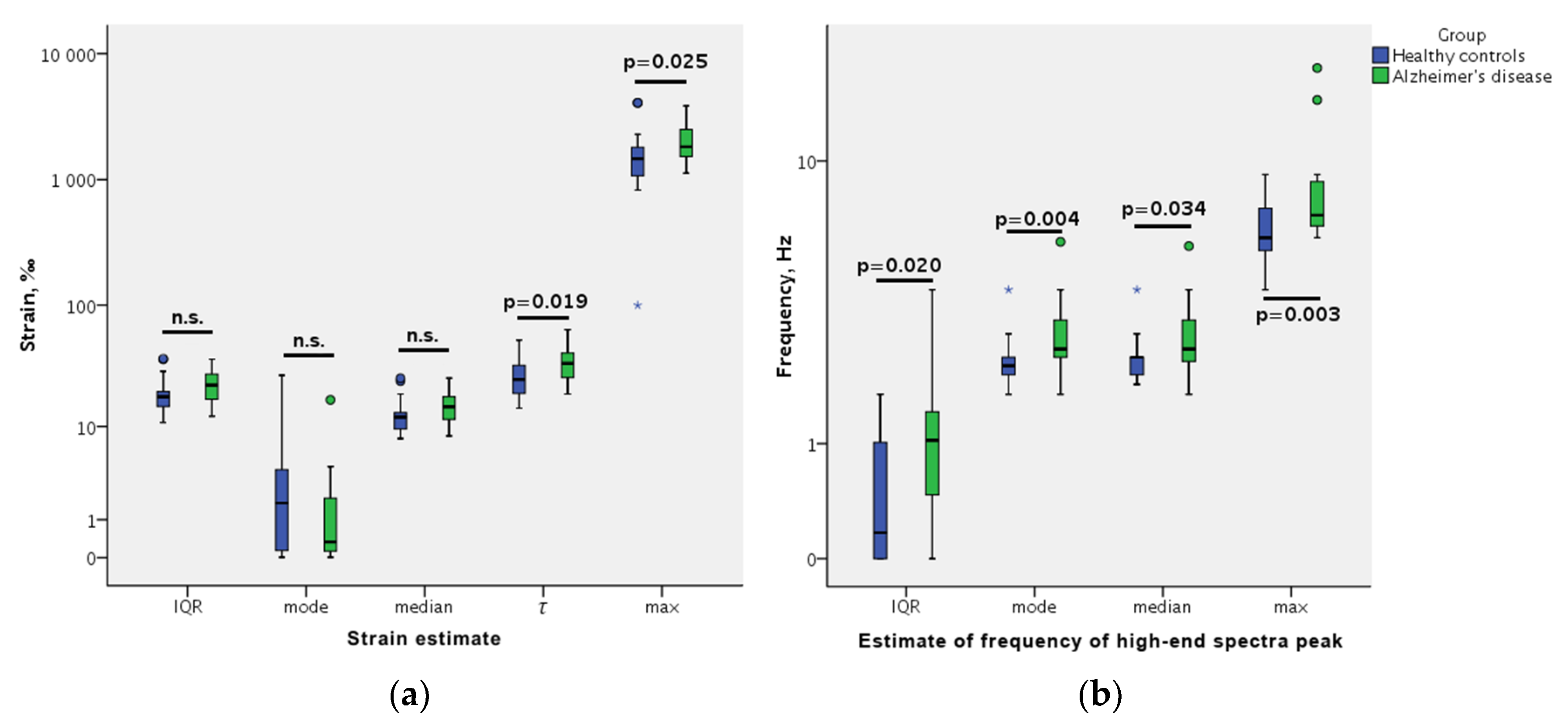
3.1. Estimates of Particular Parameters of Displacement
3.2. Models of Logistic Regression Analysis
4. Discussion
5. Conclusion
Author Contributions
Funding
Acknowledgments
Conflicts of Interest
Abbreviations
| AD | Alzheimer’s disease |
| AUC | area under a curve |
| CSF | cerebrospinal fluid |
| IQR | interquartile range |
| FreqD | dominant frequency |
| FreqHP | frequency of high-end spectra peak |
| LR | logistic regression |
| MMSE | Mini-mental state examination |
| MRI | magnetic resonance imaging |
| MTL | medial temporal lobe |
| PET | positron emission tomography |
| RF | radiofrequency |
| ROI | region of interest |
| ROC | receiver operating characteristic |
| RMS | root mean square |
| TCS | transcranial sonography |
| US | ultrasound |
References
- Nichols, E.; Szoeke, C.E.I.; Vollset, S.E.; Abbasi, N.; Abd-Allah, F.; Abdela, J.; Aichour, M.T.E.; Akinyemi, R.O.; Alahdab, F.; Asgedom, S.W.; et al. Global, regional, and national burden of Alzheimer’s disease and other dementias, 1990–2016: A systematic analysis for the Global Burden of Disease Study 2016. Lancet Neurol. 2019, 18, 88–106. [Google Scholar] [CrossRef] [Green Version]
- Frisoni, G.B.; Bocchetta, M.; Chételat, G.; Rabinovici, G.D.; de Leon, M.J.; Kaye, J.; Reiman, E.M.; Scheltens, P.; Barkhof, F.; Black, S.E.; et al. Imaging markers for Alzheimer disease: Which vs how. Neurology 2013, 81, 487–500. [Google Scholar] [CrossRef]
- Jovicich, J.; Barkhof, F.; Babiloni, C.; Herholz, K.; Mulert, C.; Berckel, B.N.M.; Frisoni, G.B. SRA-NED JPND Working Group Harmonization of neuroimaging biomarkers for neurodegenerative diseases: A survey in the imaging community of perceived barriers and suggested actions. Alzheimers Dement. Diagn. Assess. Dis. Monit. 2019, 11, 69–73. [Google Scholar] [CrossRef]
- Berg, D.; Behnke, S.; Seppi, K.; Godau, J.; Lerche, S.; Mahlknecht, P.; Liepelt-Scarfone, I.; Pausch, C.; Schneider, N.; Gaenslen, A.; et al. Enlarged hyperechogenic substantia nigra as a risk marker for Parkinson’s disease: SN+ A Risk Marker for PD. Mov. Disord. 2013, 28, 216–219. [Google Scholar] [CrossRef] [PubMed]
- Sakalauskas, A.; Speckauskiene, V.; Lauckaite, K.; Jurkonis, R.; Rastenyte, D.; Lukosevicius, A. Transcranial Ultrasonographic Image Analysis System for Decision Support in Parkinson Disease. J. Ultrasound Med. 2018, 37, 1753–1761. [Google Scholar] [CrossRef] [PubMed]
- Kallmann, B.-A.; Sauer, J.; Schließer, M.; Warmuth-Metz, M.; Flachenecker, P.; Becker†, G.; Rieckmann, P.; Mäurer, M. Determination of ventricular diameters in multiple sclerosis patients with transcranial sonography (TCS): A two year follow-up study. J. Neurol. 2004, 251, 30–34. [Google Scholar] [CrossRef] [PubMed]
- DeCarli, C. Qualitative Estimates of Medial Temporal Atrophy as a Predictor of Progression from Mild Cognitive Impairment to Dementia. Arch. Neurol. 2007, 64, 108. [Google Scholar] [CrossRef] [PubMed]
- Urs, R.; Potter, E.; Barker, W.; Appel, J.; Loewenstein, D.A.; Zhao, W.; Duara, R. Visual Rating System for Assessing Magnetic Resonance Images: A Tool in the Diagnosis of Mild Cognitive Impairment and Alzheimer Disease. J. Comput. Assist. Tomogr. 2009, 33, 73–78. [Google Scholar] [CrossRef]
- Cavallin, L.; Løken, K.; Engedal, K.; Øksengård, A.-R.; Wahlund, L.-O.; Bronge, L.; Axelsson, R. Overtime reliability of medial temporal lobe atrophy rating in a clinical setting. Acta Radiol. 2012, 53, 318–323. [Google Scholar] [CrossRef]
- Jack, C.R. Alzheimer Disease: New Concepts on Its Neurobiology and the Clinical Role Imaging Will Play. Radiology 2012, 263, 344–361. [Google Scholar] [CrossRef]
- Yilmaz, R.; Pilotto, A.; Roeben, B.; Preische, O.; Suenkel, U.; Heinzel, S.; Metzger, F.G.; Laske, C.; Maetzler, W.; Berg, D. Structural Ultrasound of the Medial Temporal Lobe in Alzheimer’s Disease. Ultraschall Med. Eur. J. Ultrasound 2017, 38, 294–300. [Google Scholar] [CrossRef] [PubMed]
- Kucewicz, J.C.; Dunmire, B.; Leotta, D.F.; Panagiotides, H.; Paun, M.; Beach, K.W. Functional Tissue Pulsatility Imaging of the Brain During Visual Stimulation. Ultrasound Med. Biol. 2007, 33, 681–690. [Google Scholar] [CrossRef] [Green Version]
- Ince, J.; Alharbi, M.; Minhas, J.S.; Chung, E.M. Ultrasound measurement of brain tissue movement in humans: A systematic review. Ultrasound 2020, 28, 70–81. [Google Scholar] [CrossRef] [PubMed]
- Selbekk, T.; Bang, J.; Unsgaard, G. Strain processing of intraoperative ultrasound images of brain tumours: Initial results. Ultrasound Med. Biol. 2005, 31, 45–51. [Google Scholar] [CrossRef] [PubMed]
- Hall, C.M.; Moeendarbary, E.; Sheridan, G.K. Mechanobiology of the brain in ageing and Alzheimer’s disease. Eur. J. Neurosci. 2020. [Google Scholar] [CrossRef] [PubMed]
- Liao, J.; Yang, H.; Yu, J.; Liang, X.; Chen, Z. Progress in the Application of Ultrasound Elastography for Brain Diseases. J. Ultrasound Med. 2020. [Google Scholar] [CrossRef]
- Varghese, T. Quasi-Static Ultrasound Elastography. Ultrasound Clin. 2009, 4, 323–338. [Google Scholar] [CrossRef] [Green Version]
- Chakraborty, A.; Berry, G.; Bamber, J.; Dorward, N. Intra-operative Ultrasound Elastography and Registered Magnetic Resonance Imaging of Brain Tumours: A Feasibility Study. Ultrasound 2006, 14, 43–49. [Google Scholar] [CrossRef]
- Kucewicz, J.C.; Dunmire, B.; Giardino, N.D.; Leotta, D.F.; Paun, M.; Dager, S.R.; Beach, K.W. Tissue Pulsatility Imaging of Cerebral Vasoreactivity During Hyperventilation. Ultrasound Med. Biol. 2008, 34, 1200–1208. [Google Scholar] [CrossRef] [Green Version]
- Jurkonis, R.; Makūnaitė, M.; Baranauskas, M.; Lukoševičius, A.; Sakalauskas, A.; Matijošaitis, V.; Rastenytė, D. Quantification of Endogenous Brain Tissue Displacement Imaging by Radiofrequency Ultrasound. Diagnostics 2020, 10, 57. [Google Scholar] [CrossRef] [Green Version]
- Michaeli, D.; Rappaport, Z.H. Tissue resonance analysis: A novel method for noninvasive monitoring of intracranial pressure: Technical note. J. Neurosurg. 2002, 96, 1132–1137. [Google Scholar] [CrossRef] [PubMed]
- Alperin, N.; Vikingstad, E.M.; Gomez-Anson, B.; Levin, D.N. Hemodynamically independent analysis of cerebrospinal fluid and brain motion observed with dynamic phase contrast MRI. Magn. Reson. Med. 1996, 35, 741–754. [Google Scholar] [CrossRef] [PubMed]
- Balédent, O.; Fin, L.; Khuoy, L.; Ambarki, K.; Gauvin, A.-C.; Gondry-Jouet, C.; Meyer, M.-E. Brain hydrodynamics study by phase-contrast magnetic resonance imaging and transcranial color doppler. J. Magn. Reson. Imaging 2006, 24, 995–1004. [Google Scholar] [CrossRef]
- Nag, D.S.; Sahu, S.; Swain, A.; Kant, S. Intracranial pressure monitoring: Gold standard and recent innovations. World J. Clin. Cases 2019, 7, 1535–1553. [Google Scholar] [CrossRef]
- Takizawa, H.; Gabra-Sanders, T.; Miller, J.D. Changes of frequency spectrum of the CSF pulse wave caused by supratentorial epidural brain compression. J. Neurol. Neurosurg. Psychiatr. 1986, 49, 1367–1373. [Google Scholar] [CrossRef] [PubMed] [Green Version]
- Robertson, C.S.; Narayan, R.K.; Contant, C.F.; Grossman, R.G.; Gokaslan, Z.L.; Pahwa, R.; Caram, P.; Bray, R.S.; Sherwood, A.M. Clinical experience with a continuous monitor of intracranial compliance. J. Neurosurg. 1989, 71, 673–680. [Google Scholar] [CrossRef] [Green Version]
- Piper, I.R.; Miller, J.D.; Dearden, N.M.; Leggate, J.R.; Robertson, I. Systems analysis of cerebrovascular pressure transmission: An observational study in head-injured patients. J. Neurosurg. 1990, 73, 871–880. [Google Scholar] [CrossRef]
- Holm, S.; Eide, P.K. The frequency domain versus time domain methods for processing of intracranial pressure (ICP) signals. Med. Eng. Phys. 2008, 30, 164–170. [Google Scholar] [CrossRef]
- Wagshul, M.E.; Eide, P.K.; Madsen, J.R. The pulsating brain: A review of experimental and clinical studies of intracranial pulsatility. Fluids Barriers CNS 2011, 8, 5–23. [Google Scholar] [CrossRef] [Green Version]
- Kasprowicz, M.; Lalou, D.A.; Czosnyka, M.; Garnett, M.; Czosnyka, Z. Intracranial pressure, its components and cerebrospinal fluid pressure-volume compensation. Acta Neurol. Scand. 2016, 134, 168–180. [Google Scholar] [CrossRef]
- Lang, E.W.; Paulat, K.; Witte, C.; Zolondz, J.; Mehdorn, H.M. Noninvasive intracranial compliance monitoring: Technical note and clinical results. J. Neurosurg. 2003, 98, 214–218. [Google Scholar] [CrossRef] [PubMed] [Green Version]
- Zhu, D.C.; Xenos, M.; Linninger, A.A.; Penn, R.D. Dynamics of lateral ventricle and cerebrospinal fluid in normal and hydrocephalic brains. J. Magn. Reson. Imaging 2006, 24, 756–770. [Google Scholar] [CrossRef] [PubMed]
- Weaver, J.B.; Pattison, A.J.; McGarry, M.D.; Perreard, I.M.; Swienckowski, J.G.; Eskey, C.J.; Lollis, S.S.; Paulsen, K.D. Brain mechanical property measurement using MRE with intrinsic activation. Phys. Med. Biol. 2012, 57, 7275–7287. [Google Scholar] [CrossRef] [PubMed] [Green Version]
- Scheltens, P.; Leys, D.; Barkhof, F.; Huglo, D.; Weinstein, H.C.; Vermersch, P.; Kuiper, M.; Steinling, M.; Wolters, E.C.; Valk, J. Atrophy of medial temporal lobes on MRI in “probable” Alzheimer’s disease and normal ageing: Diagnostic value and neuropsychological correlates. J. Neurol. Neurosurg. Psychiatr. 1992, 55, 967–972. [Google Scholar] [CrossRef] [PubMed]
- McKhann, G.; Drachman, D.; Folstein, M.; Katzman, R.; Price, D.; Stadlan, E.M. Clinical diagnosis of Alzheimer’s disease: Report of the NINCDS-ADRDA Work Group under the auspices of Department of Health and Human Services Task Force on Alzheimer’s Disease. Neurology 1984, 34, 939–944. [Google Scholar] [CrossRef] [PubMed] [Green Version]
- Ternifi, R.; Cazals, X.; Desmidt, T.; Andersson, F.; Camus, V.; Cottier, J.-P.; Patat, F.; Remenieras, J.-P. Ultrasound Measurements of Brain Tissue Pulsatility Correlate with the Volume of MRI White-Matter Hyperintensity. J. Cereb. Blood Flow Metab. 2014, 34, 942–944. [Google Scholar] [CrossRef] [Green Version]
- Desmidt, T.; Brizard, B.; Dujardin, P.-A.; Ternifi, R.; Réméniéras, J.-P.; Patat, F.; Andersson, F.; Cottier, J.-P.; Vierron, E.; Gissot, V.; et al. Brain Tissue Pulsatility is Increased in Midlife Depression: A Comparative Study Using Ultrasound Tissue Pulsatility Imaging. Neuropsychopharmacology 2017, 42, 2575–2582. [Google Scholar] [CrossRef]
- Maurice, R.L.; Bertrand, M. Lagrangian speckle model and tissue-motion estimation-theory [ultrasonography]. IEEE Trans. Med. Imaging 1999, 18, 593–603. [Google Scholar] [CrossRef]
- Ophir, J.; Céspedes, I.; Ponnekanti, H.; Yazdi, Y.; Li, X. Elastography: A quantitative method for imaging the elasticity of biological tissues. Ultrason. Imaging 1991, 13, 111–134. [Google Scholar] [CrossRef]
- Wells, P.N.T.; Liang, H.-D. Medical ultrasound: Imaging of soft tissue strain and elasticity. J. R. Soc. Interface 2011, 8, 1521–1549. [Google Scholar] [CrossRef] [Green Version]
- D’hooge, J.; Heimdal, A.; Jamal, F.; Kukulski, T.; Bijnens, B.; Rademakers, F.; Hatle, L.; Suetens, P.; Sutherland, G.R. Regional Strain and Strain Rate Measurements by Cardiac Ultrasound: Principles, Implementation and Limitations. Eur. J. Echocardiogr. 2000, 1, 154–170. [Google Scholar] [CrossRef] [PubMed] [Green Version]
- El-Khuffash, A.; Schubert, U.; Levy, P.T.; Nestaas, E.; de Boode, W.P. Deformation imaging and rotational mechanics in neonates: A guide to image acquisition, measurement, interpretation, and reference values. Pediatr. Res. 2018, 84, 30–45. [Google Scholar] [CrossRef] [Green Version]
- Zeng, W.; Gordon-Wylie, S.W.; Tan, L.; Solamen, L.; McGarry, M.D.J.; Weaver, J.B.; Paulsen, K.D. Nonlinear Inversion MR Elastography With Low-Frequency Actuation. IEEE Trans. Med. Imaging 2020, 39, 1775–1784. [Google Scholar] [CrossRef] [PubMed]
- Lacouture, Y.; Cousineau, D. How to use MATLAB to fit the ex-Gaussian and other probability functions to a distribution of response times. Tutor. Quant. Methods Psychol. 2008, 4, 35–45. [Google Scholar] [CrossRef]
- Marmolejo-Ramos, F.; González-Burgos, J. A Power Comparison of Various Tests of Univariate Normality on Ex-Gaussian Distributions. Methodology 2013, 9, 137–149. [Google Scholar] [CrossRef]
- Stone, J.; Johnstone, D.M.; Mitrofanis, J.; O’Rourke, M. The Mechanical Cause of Age-Related Dementia (Alzheimer’s Disease): The Brain is Destroyed by the Pulse. J. Alzheimers Dis. 2015, 44, 355–373. [Google Scholar] [CrossRef]
- de Montgolfier, O.; Thorin-Trescases, N.; Thorin, E. Pathological Continuum from the Rise in Pulse Pressure to Impaired Neurovascular Coupling and Cognitive Decline. Am. J. Hypertens. 2020, 33, 375–390. [Google Scholar] [CrossRef]
- Climie, R.E.; Gallo, A.; Picone, D.S.; Di Lascio, N.; van Sloten, T.T.; Guala, A.; Mayer, C.C.; Hametner, B.; Bruno, R.M. Measuring the Interaction Between the Macro- and Micro-Vasculature. Front. Cardiovasc. Med. 2019, 6, 169. [Google Scholar] [CrossRef] [Green Version]
- Goto, T.; Furihata, K.; Hongo, K. Natural resonance frequency of the brain depends on only intracranial pressure: Clinical research. Sci. Rep. 2020, 10, 2526. [Google Scholar] [CrossRef]
- Ozturk, A.; Grajo, J.R.; Dhyani, M.; Anthony, B.W.; Samir, A.E. Principles of ultrasound elastography. Abdom. Radiol. 2018, 43, 773–785. [Google Scholar] [CrossRef]
- Chatelin, S.; Constantinesco, A.; Willinger, R. Fifty years of brain tissue mechanical testing: From in vitro to in vivo investigations. Biorheology 2010, 47, 255–276. [Google Scholar] [CrossRef] [PubMed]

| Parameter Estimate | AUC, % | 95% Confidence Interval | Cut-Off | Sensitivity, % | Specificity, % |
|---|---|---|---|---|---|
| FreqHP max, Hz | 77.2 | 62.6–91.8 | 6.26 | 89.5 | 61.9 |
| FreqHP mode, Hz | 75.9 | 60.3–91.6 | 2.45 | 63.2 | 81.0 |
| FreqHP median, Hz | 69.7 | 52.7–86.6 | 2.45 | 57.9 | 76.2 |
| FreqHP IQR, Hz | 71.9 | 55.6–88.3 | 0.76 | 73.7 | 66.7 |
| Strain ex-Gaussian τ, ‰ | 71.7 | 55.9–87.5 | 23.22 | 94.7 | 42.9 |
| Strain max, ‰ | 70.7 | 54.4–87.0 | 1308.07 | 94.7 | 42.9 |
| Strain mode, ‰ | 61.7 | 44.2–79.1 | 1.58 | 73.7 | 52.4 |
| Parameter Estimate | β | Exp(β) | Exp(β) 95% Confidence Interval | p Value |
|---|---|---|---|---|
| 1st Model | ||||
| FreqHP_IQR | 2.396 | 10.976 | 1.021–117.985 | 0.048 |
| FreqHP_mode | 4.599 | 99.424 | 3.312–2984.675 | 0.008 |
| FreqHP_max | 1.196 | 3.306 | 1.040–10.506 | 0.043 |
| Strain_mode | −0.510 | 0.600 | 0.390–0.926 | 0.021 |
| Constant | −19.838 | <0.001 | - | 0.002 |
| 2nd Model | ||||
| FreqHP_IQR | 2.377 | 10.776 | 0.969–119.885 | 0.053 |
| FreqHP_mode | 4.455 | 86.028 | 2.744–2696.678 | 0.011 |
| FreqHP_max | 1.144 | 3.138 | 1.026–9.597 | 0.045 |
| Strain_mode | −0.498 | 0.607 | 0.392–0.942 | 0.026 |
| Age | 0.040 | 1.041 | 0.852–1.272 | 0.696 |
| Constant | −21.989 | <0.001 | - | 0.013 |
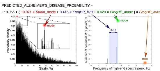
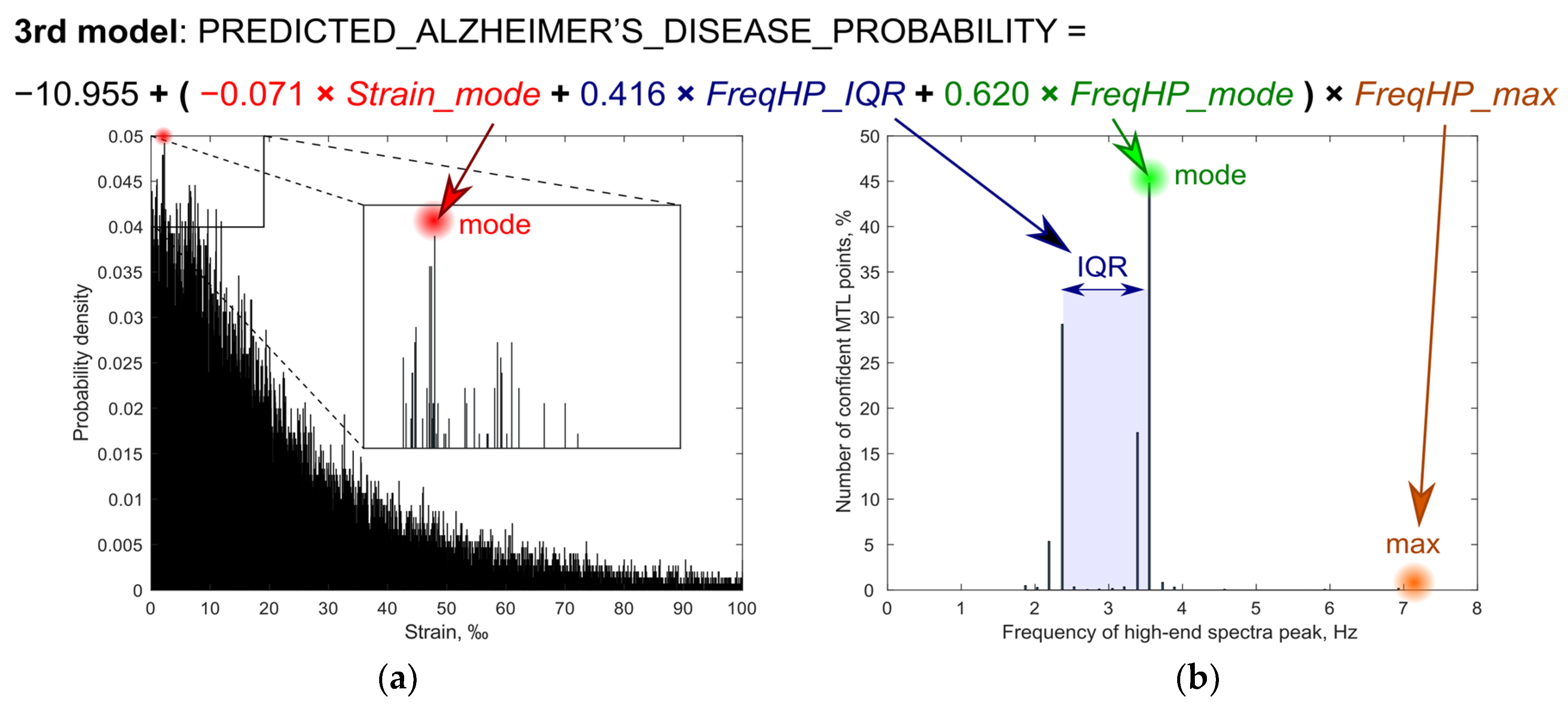
| 3rd Model | ||||
| FreqHP_IQR × FreqHP_max | 0.416 | 1.516 | 1.025 2.240 | 0.037 |
| FreqHP_mode × FreqHP_max | 0.620 | 1.859 | 1.216–2.841 | 0.004 |
| Strain_mode × FreqHP_max | −0.071 | 0.931 | 0.879–0.987 | 0.016 |
| Constant | −10.955 | <0.001 | - | 0.002 |
| 4th Model | ||||
| FreqHP_IQR × FreqHP_max | 0.410 | 1.507 | 1.015–2.235 | 0.042 |
| FreqHP_mode × FreqHP_max | 0.600 | 1.821 | 1.181–2.809 | 0.007 |
| Strain_mode × FreqHP_max | −0.069 | 0.933 | 0.880–0.989 | 0.020 |
| Age | 0.027 | 1.028 | 0.841–1.255 | 0.789 |
| Constant | −12.573 | <0.001 | - | 0.082 |
| Predicted Probability in Model | AUC, % | p Value | 95% Confidence Interval | Cut-Off, % | Sensitivity, % | Specificity, % |
|---|---|---|---|---|---|---|
| 1st model | 95.5 | <0.001 | 88.6–100.0 | 60.98 | 89.5 | 100.0 |
| 2nd model | 95.2 | <0.001 | 87.9–100.0 | 66.53 | 89.5 | 100.0 |
| 3rd model | 95.5 | <0.001 | 88.3–100.0 | 65.20 | 89.5 | 100.0 |
| 4th model | 95.7 | <0.001 | 88.7–100.0 | 68.47 | 89.5 | 100.0 |
© 2020 by the authors. Licensee MDPI, Basel, Switzerland. This article is an open access article distributed under the terms and conditions of the Creative Commons Attribution (CC BY) license (http://creativecommons.org/licenses/by/4.0/).
Share and Cite
Baranauskas, M.; Jurkonis, R.; Lukoševičius, A.; Makūnaitė, M.; Matijošaitis, V.; Gleiznienė, R.; Rastenytė, D. Ultrasonic Assessment of the Medial Temporal Lobe Tissue Displacements in Alzheimer’s Disease. Diagnostics 2020, 10, 452. https://doi.org/10.3390/diagnostics10070452
Baranauskas M, Jurkonis R, Lukoševičius A, Makūnaitė M, Matijošaitis V, Gleiznienė R, Rastenytė D. Ultrasonic Assessment of the Medial Temporal Lobe Tissue Displacements in Alzheimer’s Disease. Diagnostics. 2020; 10(7):452. https://doi.org/10.3390/diagnostics10070452
Chicago/Turabian StyleBaranauskas, Mindaugas, Rytis Jurkonis, Arūnas Lukoševičius, Monika Makūnaitė, Vaidas Matijošaitis, Rymantė Gleiznienė, and Daiva Rastenytė. 2020. "Ultrasonic Assessment of the Medial Temporal Lobe Tissue Displacements in Alzheimer’s Disease" Diagnostics 10, no. 7: 452. https://doi.org/10.3390/diagnostics10070452
APA StyleBaranauskas, M., Jurkonis, R., Lukoševičius, A., Makūnaitė, M., Matijošaitis, V., Gleiznienė, R., & Rastenytė, D. (2020). Ultrasonic Assessment of the Medial Temporal Lobe Tissue Displacements in Alzheimer’s Disease. Diagnostics, 10(7), 452. https://doi.org/10.3390/diagnostics10070452