A Deep Learning-Based Automated CT Segmentation of Prostate Cancer Anatomy for Radiation Therapy Planning-A Retrospective Multicenter Study

Abstract

A commercial deep learning (DL)-based automated segmentation tool (AST) for computed tomography (CT) is evaluated for accuracy and efficiency gain within prostate cancer patients. Thirty patients from six clinics were reviewed with manual- (MC), automated- (AC) and automated and edited (AEC) contouring methods. In the AEC group, created contours (prostate, seminal vesicles, bladder, rectum, femoral heads and penile bulb) were edited, whereas the MC group included empty datasets for MC. In one clinic, lymph node CTV delineations were evaluated for interobserver variability. Compared to MC, the mean time saved using the AST was 12 min for the whole data set (46%) and 12 min for the lymph node CTV (60%), respectively. The delineation consistency between MC and AEC groups according to the Dice similarity coefficient (DSC) improved from 0.78 to 0.94 for the whole data set and from 0.76 to 0.91 for the lymph nodes. The mean DSCs between MC and AC for all six clinics were 0.82 for prostate, 0.72 for seminal vesicles, 0.93 for bladder, 0.84 for rectum, 0.69 for femoral heads and 0.51 for penile bulb. This study proves that using a general DL-based AST for CT images saves time and improves consistency.

1. Introduction

Prostate cancer is the most common cancer type among the western male population. Radiation therapy (RT) remains a cornerstone in the curative treatment chain with surgery and hormonal therapies [1,2]. Almost 1.3 million new prostate cancer cases were diagnosed worldwide in 2018, and the number is estimated to increase by 35% in 10 years and even up to 80% by 2040 [1]. Access to RT is geographically unequal, with regions in poverty having longer waiting times and less access to lifesaving RT globally and locally [1,3]. As the number of cancer patients treated with ionizing radiation increases, healthcare services have to manage limited financial and human resources, indicating a need for automated solutions and tools.

High geometric and dosimetric accuracy are critical for successful RT. Wide use of image- and surface-guided radiation therapy (IGRT, SGRT) and target tracking methods ensure accurate treatment targeting and reproducibility of patient positioning. Correspondingly, recent increases in using volumetric- or intensity-modulated radiation therapy (VMAT, IMRT) and stereotactic body radiation therapy (SBRT) have enabled us to shape the dose distributions much more accurately to match the treatment target and minimize the dose to organs at risk (OAR) [4]. However, the sharp dose gradients created by these techniques can be hazardous if the delineation of structures is inaccurate [5]. For prostate cancer, the challenges concerning inter- and intraobserver variation in target delineation have been well known for decades [6,7,8]; however, it remains the weakest link in the accuracy of RT [9].

To save clinicians’ resources, automated segmentation tools (AST) for radiation therapy planning (RTP) have been developed, ranging from adaptive thresholding to atlas-based techniques [10]. However, using such automated techniques has been limited due to the complexity of the anatomy and poor contrasts in the pelvic region in computed tomography (CT) images. In practice, the accuracy and speed of the delineation have not been good enough to ease clinicians’ work burden [11]. More recently, the focus on autosegmentation has shifted to artificial intelligence (AI)-based methods [12,13,14]. AI is a branch of computer science that attempts to emulate human-like intelligence in machines through computer software and algorithms without direct human stimuli. Deep learning (DL) is the latest form of AI concerned with artificial neural network (ANN) algorithms that mimic the human nervous system [12,15]. Each “neuron” receives an input and creates an output in successive layers, capable of weighing the importance of the passing information. DL uses multiple levels of abstraction in its process to learn connections and correlations when provided with a database. It typically requires large amounts of training data and computational resources. A trained DL model generates results accurately and quickly with minimal user interaction, and the output results directly from the learned features from the problem distribution. For the delineation of structures of interest in RTP of prostate cancer, the problem distribution is a medical imaging dataset with segmented contours [16,17,18,19].

In this study, MVision Delineation from MVision AI Oy (Helsinki, Finland), a fully automated commercially available 3D DL model, was evaluated for accuracy and efficiency gain for CT-based autocontouring for prostate cancer RTP. Conventional evaluation metrics were used to evaluate delineation accuracy between the predictions of the model and the ground truths of clinicians’ contouring.

2. Materials and Methods

2.1. DL Delineation Model

The DL model employed is a convolutional neural network based on an encoder–decoder architecture, similar to 3D U-Net [20] and with more recent residual blocks [21]. To train the DL model, ca. 900 prostate cancer patients’ planning CT image sets from three clinics were collected. Clinical contours with large outliers were excluded from the data. The data used for training the model included 876 samples for bladder, 848 for rectum, 738 for prostate, 416 for penile bulb, 222 for seminal vesicles, 212 for lymph nodes and 127 and 128 for left and right femur heads.

The same pretrained general DL-based AST model was used at all clinics in the study. It is a cloud-based system that uses pseudonymized DICOM data in the autocontouring process. Once it completes the delineations, it sends them automatically back to the clinic’s RTP system for clinicians to review, edit, and approve the results.

2.2. Study Patients

This is a retrospective institutional review board- and The Finnish Institute for Health and Welfare (Terveyden ja hyvinvoinnin laitos (THL) Helsinki, Finland) approved multicenter study. All procedures performed in the study were in accordance with the ethical standards of the institutional and/or national research committee and with the Declaration of Helsinki by the World Medical Association and its later amendments or comparable ethical standards.

Thirty prostate cancer patients were randomly selected from six clinics’ databases, concluding five patients per clinic with RTP CT images and corresponding segmentations. One clinic from Estonia (North Estonia Medical Centre, Tallinn), four clinics from Finland (Docrates Cancer Center, Kuopio University Hospital, Oulu University Hospital, Turku University Hospital) and one clinic from Singapore (National Cancer Centre Singapore) participated in the study. The selection criteria for the patients were: RTP for prostate cancer, no prostatectomy and no femoral implants. Scans were not used in the training set to create the DL model. Two GE (Lightspeed RT16), two Siemens (Sensation Open and Definition) and two Toshiba (Aquilion LB) scanners were used for CT imaging of the patients.

For a blind evaluation, the same patient scans were duplicated and anonymized to manual contouring (MC) and automated and edited contouring (AEC) groups then sent back to the clinics for delineation. Automated contouring (AC) without editions were also used for the comparison. All the regions of interest (ROI) for the AEC group were edited from the autosegmentations to reach clinically acceptable contours, whereas the MC group included empty datasets for manual contouring. Six clinics produced seven ROIs including prostate, seminal vesicles, bladder, rectum, femoral heads and penile bulb. The lymph nodes were produced at one clinic.

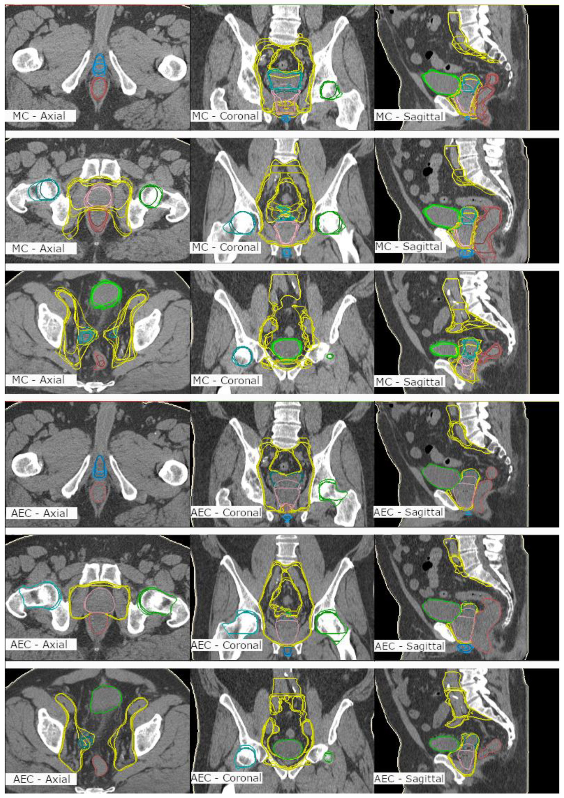
2.3. Contouring

Up to three specialists completed the delineations in each clinic except one, where four oncologists delineated the same 5 patients’ datasets (20 scans altogether) so the interobserver variability could be assessed within the clinic. In this clinic, lymph nodes’ CTV delineations were also evaluated. The analyzed dataset therefore consisted of 30 patients and 45 scans. The OARs were contoured according to each clinic’s clinical protocol either by an oncologist, dosimetrist, radiotherapy technologist or physicist. Contouring was completed in two phases. First, the MC was done by measuring the total time taken for the task per patient. All semiautomatic segmentation tools (such as deformable brush, autothreshold, autopilot, etc.), which were clinically used, could be used for contouring. An RTP system Eclipse (v15.6, Varian Medical Systems Finland Oy, Helsinki, Finland) was used at the Docrates Cancer Center, National Cancer Centre Singapore, Oulu University Hospital and Turku University Hospital for the MC or semiautomatic contouring. Elekta Monaco (v5.11, Elekta Instrument AB, Stockholm, Sweden) was used at the North Estonia Medical Centre and MIM Software (v6.9, MIM Software Inc., Cleveland, OH, USA) at Kuopio University Hospital. A minimum interval of one week was introduced after the MC to minimize possible learning and memory trace of individual patient contouring. Secondly, the same specialists evaluated the autocontouring results, edited the contours until clinically acceptable and measured the total time spent per patient. By the end of phase two, three groups of contours were collected for analysis:

• An MC group contoured in the study into an empty dataset to meet clinical acceptance.
• An AC group that included the nonedited automatically created structure set.
• An AEC group that included the automatically created structures with expert modifications to meet clinical acceptance.

2.4. Contouring Analysis

Efficiency gain using the AST was measured by comparing the total contouring times per patient of the MC method and AEC method to reach clinically acceptable contours. Accuracy of the AST was measured by comparing the AC delineation with all MC delineations with the Dice similarity coefficient (DSC), surface Dice similarity coefficient (S-DSC), 95% Hausdorff distance (HD95) and difference in absolute and relative volume (Diff_mm3 and Diff_%). DSC is the most common metric used to compare binary segmentation masks. It is the ratio of the overlap between two masks normalized by their size, and its value ranges between 0 (no overlap) and 1 (perfect overlap). S-DSC [22] measures the proportion of the surfaces of two masks that lie within a given tolerance (in mm) from each other. We used a fixed tolerance of 2.5 mm for all structures. HD is the maximum distance between the surfaces of two masks. Since HD is very sensitive to outliers, we used HD95, which is the 95th percentile of the distances between the surfaces of the masks. Diff_mm3 is the absolute volume difference between the two masks in mm3 and Diff_% is the relative volume difference between the two masks. The similarity metrics were calculated by an in-house developed (Python) code.

Interobserver consistency using the MC method and AEC method was measured in two ROI groups: first, by comparing the produced lymph node segmentations and second, by comparing five ROIs, including the bladder, prostate, penile bulb, rectum and seminal vesicles, by four oncologists on five patients’ CT scans (the same scans for each oncologist) with both methods. Interobserver consistency was determined by calculating the DSCs of each oncologist compared with the other three oncologists.

3. Results

The efficiency gain in ROI segmentation time using the AST is shown in Figure 1. In all clinics, the average absolute and relative time saved ranged from 0.6 to 17 min and from 1.5% to 70.9%, respectively. Over the expert observers, the absolute and relative time saved ranged from −5 to 51 min and from −25.8% to 96.2%, respectively. The overall average relative time saved for 13 experts contouring 30 patients and 45 scans was 45.8% using the AST. The overall mean absolute MC and AEC delineation times were 27 and 15 min, respectively. For the lymph node delineation, the mean delineation time between four oncologists decreased by 60% from 20 (MC) to 8 min (AEC).

The overall performance of AST is reported in

Table 1. Average similarity scores (DSC, S-DSC and HD95) and average absolute and relative volume differences with one standard deviation (Diff_cm3 and Diff %) between manual contouring (MC) and automated contouring (AC) methods from 30 patients and 45 scans in six clinics by 13 experts.

ROI	DSC	S-DSC (2.5 mm)	HD95 (mm)	Diff_cm3 (cm3)	Diff_% (%)
Bladder	0.93	0.68	3.3	−1.2 ± 12.0	−1.7 ± 8.3
Prostate	0.82	0.38	6.1	−13.5 ± 10.1	−31.6 ± 26.1
Femoral head L	0.68	0.22	25.0	−4.0 ± 32.4	−37.9 ± 60.7
Femoral head R	0.69	0.22	24.7	−3.0 ± 31.2	−30.5 ± 38.7
Lymph nodes *	0.80	0.39	14.7	40.9 ± 86.3	5.2 ± 12.4
Penile bulb	0.51	0.33	7.7	1.2 ± 2.2	−6.8 ± 67.0
Rectum	0.84	0.58	11.4	−4.5 ± 11.4	−9.6 ± 18.7
Seminal vesicles	0.72	0.52	7.1	0.6 ± 6.9	−11.1 ± 31.2

* The lymph nodes were evaluated for five patients and 20 scans while it was performed in one clinic only. ROI: regions of interest, DSC: Dice similarity coefficient, S-DSC: surface Dice similarity coefficient, HD95: 95% Hausdorff distance, L: left, R: right.

in terms of similarity metrics between AC and MC. As seen for the relative volume difference of femoral heads, the results are compromised due to the style differences between the style of the AST and the clinical practice.

The interobserver consistency was studied between the MC and AEC methods by determining the similarity metrics between four experienced oncologists in Clinic 1. The quantitative results are shown in

Table 2. Dice similarity coefficients (DSC) were evaluated between four oncologists for the same five patient data set for manual contouring (MC) and automated and edited contouring (AEC) method. Diff = DSC difference between AEC and MC methods (ROI: regions of interest).

		Oncologist 2			Oncologist 3			Oncologist 4
	ROI	AEC	MC	Diff	AEC	MC	Diff	AEC	MC	Diff
Oncologist 1	Bladder	1.00	0.90	0.10	1.00	0.92	0.08	1.00	0.91	0.09
	Prostate	0.92	0.82	0.10	0.99	0.83	0.17	1.00	0.86	0.14
	Lymph nodes	0.88	0.74	0.14	0.89	0.78	0.12	0.95	0.81	0.14
	Penile bulb	0.82	0.56	0.26	0.87	0.71	0.15	0.80	0.66	0.14
	Rectum	0.97	0.74	0.23	0.97	0.77	0.19	0.98	0.82	0.16
	Seminal vesicles	0.84	0.78	0.06	0.97	0.75	0.22	0.97	0.74	0.24
Oncologist 2	Bladder				1.00	0.91	0.08	1.00	0.92	0.08
	Prostate				0.92	0.86	0.06	0.92	0.80	0.12
	Lymph nodes				0.87	0.78	0.10	0.91	0.72	0.19
	Penile bulb				0.82	0.57	0.24	0.90	0.61	0.29
	Rectum				0.99	0.64	0.35	0.99	0.76	0.23
	Seminal vesicles				0.84	0.79	0.05	0.83	0.79	0.04
Oncologist 3	Bladder							1.00	0.92	0.08
	Prostate							0.99	0.82	0.18
	Lymph nodes							0.92	0.74	0.18
	Penile bulb							0.80	0.74	0.06
	Rectum							0.99	0.77	0.22
	Seminal vesicles							0.97	0.77	0.20

for all organs as a five-patients average DSC. For the lymph nodes, the AEC produced higher interobserver consistency between four oncologists when compared with the MC with overall average DSCs of 0.91 ± 0.04 and 0.76 ± 0.04, respectively. For other ROIs, this was consistently evident as well, with overall average DSCs of 0.94 ± 0.06 and 0.78 ± 0.05. The qualitative results may be seen in Figure 2 for all ROIs. By inspecting the resulting ROI segmentations by the four oncologists in Figure 2, one may note better interobserver consistency produced by the AEC than that of the MC, especially for large and challenging ROI, such as the lymph nodes, as confirmed in Table 2.

4. Discussion

This study emphasizes that DL-based AST streamlines the workload in clinics and decreases the delineation variability between specialists in clinics. The mean time saved was 12 min or 46% for the full set of prostate RTP contours for six clinics and 12 min or 60% when the regional lymph nodes were also included for RTP at one clinic.

In earlier publications, study groups performed similar studies with 5–20 patients [23,24,25,26,27,28]. As we did not have previous data to evaluate a sufficient sample size for the study using power calculation, we used a greater sample size of 30 patients or 45 scans. Langmack et al. [27] presented an equal delineation time using an atlas-based system for prostate RTP. The mean delineation times for manual and automated segmentations were 27 and 16 min, respectively. However, the atlas-based delineation failed in the delineation of seminal vesicles (DSC of 0.57–0.58) and was only moderate for rectum (DSC of 0.76–0.79), which both are critical organs for the RTP of prostate cancer. In a multicenter study, delineation variation is usually larger than in a more focused or single-center study. Still, our DCSs were consistently higher compared with Langmack’s results, except for femoral heads, where the contour style in the trained model was different when compared with individual clinics. Sjöberg et al. [28] evaluated atlas-based pelvic lymph node delineation and found 23–35% (4–6 min) of mean time saved per patient, which was less than half of the time saved compared with our study for the lymph nodes with 49–75% (10–16 min) of time saved.

Balagopal et al. [16] presented a similar DSC for the DL-based autosegmentation of bladder (0.95) and rectum (0.84). Their DSCs were better for prostate (0.90) and femoral heads (0.95–0.96), but they used only one observer and one CT device as a reference, which would have biased the results if compared with a multicenter study. Their model did not delineate seminal vesicles or penile bulb. Magnetic resonance imaging (MRI) is increasingly used in the RTP of prostate cancer to reduce the uncertainty of target volume delineation. Very recently, Kuisma et al. [29] presented results of a commercial-model-based AST for MRI. In their single-center and single-observer study, the DSCs were similar as in our multicenter CT-based study for prostate (0.82 vs. 0.84), bladder (0.93 vs. 0.92) and rectum (0.84 vs. 0.86). Our model was superior for seminal vesicles (0.72 vs. 0.56) but inferior for penile bulb (0.51 vs. 0.69). MRI has a better soft-tissue contrast compared with CT, which might partly explain the better penile bulb DSCs in MRI. In addition, DSC is strongly affected by the size of the structure, which partly explains poor values for smaller structures, such as the penile bulb.

We added different similarity metrics in Table 1 to make it easier in the future for the research community to compare the similarity metrics between large and small ROIs. The S-DSC measures the segmentation accuracy in relation to the contour lines overlapping rather than the overlapping of the volumes, where the volumes of the ROIs will have a large impact on the DSC, contrary to S-DSC. Examples of this are the DSC of 0.69 and S-DSC of 0.22 for femurs and the DSC of 0.51 and S-DSC of 0.33 for penile bulb. The DSC score decreases more with smaller-volume penile bulb compared with larger-volume femurs, although the contour line overlap is larger for penile bulb than for femurs, as shown by S-DSC. The average relative volume difference between the MC and AC methods for penile bulb and femurs were 6.8% and 34.2%, respectively.

Delineation consistency between the clinics was not possible to evaluate since each clinic only delineated their own patients. However, the interobserver variation was evaluated at one clinic between four experienced oncologists. The consistency increased with the AEC method, as the DSCs for the lymph nodes were 0.76 and 0.91 for the MC and AEC, respectively. The increased consistency is also qualitatively visible in Figure 2, where MC and AEC are presented at three planes. The same was evident for the other organs as well, with overall average DSCs of 0.78 ± 0.05 and 0.94 ± 0.06 for the MC and AEC methods, respectively. The improved consistency will have a great impact in large hospitals with several specialists to standardize treatment or to assist optimal delineation for physicians in training.

In our study, there was a large time-saved variation between the clinics. Clinics 1 and 3 saved 70–71% in the delineation time, while Clinic 6 saved only 1.5% on average. However, time saving was larger when the femurs were excluded from the analysis. For femoral heads, there was a large difference between how the AST was trained and the contouring style used in two clinics (Figure 3). This style difference had an obvious negative impact on the efficiency gain. We compared the change in efficiency gain when femoral heads were excluded from the time save analysis. Absolute and relative time saved increased from 5.6 to 8.1 min (from 10.7% to 18.4%) at Clinic 2 and from 0.5 to 4.6 min (from 1.5% to 31.3%) at Clinic 6.

Langmack et al. found that the DSC should be larger than 0.65 to save time using AST and time saving increases linearly with the DSC [27]. The mean DSC per patient in all clinics was higher than 0.60 and only in two scans below 0.65, indicating there should have been reasonable time saved in all clinics. In this study, the clinics were asked to edit the AC group such that the contours would have been clinically feasible for RTP. However, some clinics used a lot of time to edit the femoral heads, with the lowest DSC of 0.38, which were not autosegmented according to their clinical protocol. This deteriorated the total delineation time but did not have a clinical impact on the RTP. On both occasions, the femoral heads’ doses would have been neglected (V50Gy << 5%, the radiation therapy oncology group (RTOG) consensus) [30]. The current version of the model follows the ESTRO ACROP consensus guidelines [31], where the femurs are similar to the style on the right in Figure 3. In a new clinic that is starting to use DL-based delineation, there is a learning curve to accommodate a new way of working. To overcome this, the model should also be able to adapt to certain local delineation protocols. While the model is clinically used for autosegmentation, the model could also learn from the clinically edited contours to correspond to the clinic’s way of working. A national and an international contouring database would fully overcome this if every clinic used the same clinical contouring protocol.

When the segmentation model is based on the latest guidelines, it would also challenge experienced specialists to review their current practices. Likewise, the model should be kept up to date. Additionally, the use of the commercial AST studied here could free up time for clinicians to tackle more important delineation tasks (dose painting, intraprostatic boost, etc.), as every contour does not have to be started from scratch. With consistent normal tissue delineation through consensus guidelines and delineation implementation with accurate ASTs across the clinics, the comparability of radiation toxicity studies could increase in the future. The DL-based AST evaluated in this study could provide a basis for improving the accuracy and consistency of the most critical step in radiation delivery to control disease and limit adverse effects related to errors in the delineation of structures in RTP of prostate cancer patients.

References

- Bray, F.; Ferlay, J.; Soerjomataram, I.; Siegel, R.L.; Torre, L.A.; Jemal, A. Global cancer statistics 2018: GLOBOCAN estimates of incidence and mortality worldwide for 36 cancers in 185 countries. Ca Cancer J. Clin. 2018, 68, 394–424. [Google Scholar] [CrossRef] [PubMed]
- Mohler, J.L.; Antonarakis, E.S.; Armstrong, A.J.; D’Amico, A.V.; Davis, B.J.; Dorff, T.; Eastham, J.A.; Enke, C.A.; Farrington, T.A.; Higano, C.S.; et al. Prostate Cancer, Version 2.2019, NCCN Clinical Practice Guidelines in Oncology. JNCCN 2019, 17, 479–505. [Google Scholar] [CrossRef] [PubMed]
- Williams, M.W.; Drinkwater, K.J. Geographical Variation in Radiotherapy Services across the UK in 2007 and the Effect of Deprivation. Clin. Oncol. 2009, 21, 431–440. [Google Scholar] [CrossRef] [PubMed]
- Moon, D.H.; Efstathiou, J.A.; Chen, R.C. What is the best way to radiate the prostate in 2016? Urol. Oncol. 2017, 35, 59–68. [Google Scholar] [CrossRef]
- Chen, A.M.; Chin, R.; Beron, P.; Yoshizaki, T.; Mikaeilian, A.G.; Cao, M. Inadequate target volume delineation and local–Regional recurrence after intensity-modulated radiotherapy for human papillomavirus-positive oropharynx cancer. Radiother. Oncol. 2017, 123, 412–418. [Google Scholar] [CrossRef]
- Cazzaniga, L.F.; Marinoni, M.A.; Bossi, A.; Bianchi, E.; Cagna, E.; Cosentino, D.; Scandolaro, L.; Valli, M.; Frigerio, M. Interphysician variability in defining the planning target volume in the irradiation of prostate and seminal vesicles. Radiother. Oncol. 1998, 47, 293–296. [Google Scholar] [CrossRef]
- Fiorino, C.; Reni, M.; Bolognesi, A.; Cattaneo, G.M.; Calandrino, R. Intra- and inter-observer variability in contouring prostate and seminal vesicles, implications for conformal treatment planning. Radiother. Oncol. 1998, 47, 285–292. [Google Scholar] [CrossRef]
- Valicenti, R.K.; Sweet, J.W.; Hauck, W.W.; Hudes, R.S.; Lee, T.; Dicker, A.P.; Waterman, F.M.; Anne, P.R.; Corn, B.W.; Galvin, J.M. Variation of clinical target volume in three-dimensional conformal radiation therapy for prostate cancer. Int. J Radiot. Oncol. Biol. Phys. 1999, 44, 931–935. [Google Scholar] [CrossRef]
- Njeh, C.F. Tumor delineation, the weakest link in the search for accuracy in radiotherapy. J. Med. Phys. 2008, 33, 136–140. [Google Scholar] [CrossRef]
- Sharp, G.; Fritscher, K.D.; Pekar, V.; Peroni, M.; Shusharina, N.; Veeraraghavan, H.; Yang, J. Vision 20/20: Perspectives on automated image segmentation for radiotherapy. Med. Phys. 2014, 41, 050902. [Google Scholar] [CrossRef]
- Geraghty, J.P.; Grogan, G.; Ebert, M.A. Automatic segmentation of male pelvic anatomy on computed tomography images: A comparison with multiple observers in the context of a multicentre clinical trial. Radiat. Oncol. 2013, 8, 106. [Google Scholar] [CrossRef] [PubMed]
- LeCun, Y.; Bengio, Y.; Hinton, G. Deep learning. Nature 2015, 521, 436–444. [Google Scholar] [CrossRef] [PubMed]
- Meyer, P.; Noblet, V.; Mazzara, C.; Lallement, A. Survey on deep learning for radiotherapy. Biol. Med. 2018, 98, 126–146. [Google Scholar] [CrossRef]
- El Naqa, I.; Ruan, D.; Valdes, G.; Dekker, A.; McNutt, T.; Ge, Y.; Wu, Q.J.; Hun Oh, J.; Thor, M.; Smith, W.; et al. Machine learning and modeling: Data, validation, communication challenges. Med. Phys. 2018, 45, e834–e840. [Google Scholar] [CrossRef] [PubMed]
- Litjens, G.; Kooi, T.; Bejnordi, B.E.; Setio, A.A.A.; Ciompi, F.; Ghafoorian, M.; van der Laak, A.W.M.J.; van Ginneken, B.; Sánchez, C.I. A survey on deep learning in medical image analysis. Med. Image Anal. 2017, 42, 60–88. [Google Scholar] [CrossRef] [PubMed]
- Balagopal, A.; Kazemifar, S.; Nguyen, D.; Lin, M.H.; Hannan, R.; Owrangi, A.; Jiang, S. Fully automated organ segmentation in male pelvic CT images. Phys. Med. Biol. 2018, 63, 245015. [Google Scholar] [CrossRef] [PubMed]
- He, K.; Cao, X.; Shi, Y.; Nie, D.; Gao, Y.; Shen, D. Pelvic Organ Segmentation Using Distinctive Curve Guided Fully Convolutional Networks. IEEE Trans. Med. Imaging 2019, 38, 585–595. [Google Scholar] [CrossRef]
- Kearney, V.; Chan, J.W.; Wang, T. Attention-enabled 3D boosted convolutional neural networks for semantic CT segmentation using deep supervision. Phys. Med. Biol. 2019, 64, 135001. [Google Scholar] [CrossRef]
- Liu, C.; Gardner, S.J.; Wen, N.; Elshaikh, M.A.; Siddiqui, F.; Movsas, B.; Chetty, I.J. Automatic Segmentation of the Prostate on CT Images Using Deep Neural Networks (DNN). Int. J. Radiat. Oncol. Biol. Phys. 2019, 104, 924–932. [Google Scholar] [CrossRef]
- Çiçek, Ö.; Abdulkadir, A.; Lienkamp, S.S.; Brox, T.; Ronneberger, O. 3D U-Net: Learning Dense Volumetric Segmentation from Sparse Annotation. arXiv 2016, arXiv:1606.06650. [Google Scholar]
- Chen, A.M.; Chin, R.; Beron, P.; Yoshizaki, T.; Mikaeilian, A.G.; Cao, M. Deep Residual Learning for Image Recognition. In Proceedings of the 2016 IEEE Conference on Computer Vision and Pattern Recognition, CVPR 2016, Las Vegas, NV, USA, 27–30 June 2016; pp. 770–778. [Google Scholar]
- Nikolov, S.; Blackwell, S.; Mendes, R.; De Fauw, J.; Meyer, C.; Hughes, C.; Patel, Y.; Meyer, C.; Askham, H.; Romera-Paredes, B.; et al. Deep learning to achieve clinically applicable segmentation of head and neck anatomy for radiotherapy. arXiv 2018, arXiv:1809.04430. [Google Scholar]
- Pejavar, S.; Yom, S.S.; Hwang, A.; Speight, J.; Gottschalk, A.; Hsu, I.C.; Roach, M., III. Computer-Assisted, Atlas-Based Segmentation for Target Volume Delineation in Whole Pelvic IMRT for Prostate Cancer. Technol. Cancer Res. Treat. 2013, 3, 199–206. [Google Scholar] [CrossRef]
- La Macchia, M.; Fellin, F.; Amichetti, M.; Cianchetti, M.; Gianolini, S.; Paola, V.; Lomax, A.J.; Widesott, L. Systematic evaluation of three different commercial software solutions for automatic segmentation for adaptive therapy in head-and-neck, prostate and pleural cancer. Radiat. Oncol. 2012, 7, 160. [Google Scholar] [CrossRef]
- Simmat, I.; Georg, P.; Georg, D.; Birkfellner, W.; Goldner, G.; Stock, M. Assessment of accuracy and efficiency of atlas-based autosegmentation for prostate radiotherapy in a variety of clinical conditions. Strahlenther. Onkol. 2012, 188, 807–815. [Google Scholar] [CrossRef] [PubMed]
- Hwee, J.; Louie, A.V.; Gaede, S.; Bauman, G.; D’Souza, D.; Sexton, T.; Lock, M.; Ahmad, B.; Rodrigues, G. Technology Assessment of Automated Atlas Based Segmentation in Prostate Bed Contouring. Radiat. Oncol. 2011, 6, 110. [Google Scholar] [CrossRef] [PubMed]
- Langmack, K.A.; Perry, C.; Sinstead, C.; Mills, J.; Saunders, D. The utility of atlas-based segmentation in the male pelvis is dependent on the interobserver agreement of the structures segmented. Br. J. Radiol. 2014, 87, 20140299. [Google Scholar] [CrossRef]
- Sjöberg, C.; Lundmark, M.; Granberg, C.; Johansson, S.; Ahnesjö, A.; Montelius, A. Clinical evaluation of multi-atlas based segmentation of lymph node regions in head and neck and prostate cancer patients. Radiat. Oncol. 2013, 8, 229. [Google Scholar] [CrossRef] [PubMed]
- Kuisma, A.; Ranta, I.; Keyriläinen, J.; Suilamo, S.; Wright, P.; Pesola, M.; Warner, L.; Löyttyniemi, E.; Minn, H. Validation of automated magnetic resonance image segmentation for radiation therapy planning in prostate cancer. PHIRO 2020, 13, 14–20. [Google Scholar] [CrossRef]
- Lawton, C.A.; Michalski, J.; El-Naqa, I.; Buyyounouski, M.K.; Lee, W.R.; Menard, C.; O’Meara, M.D.E.; Rosenthal, S.A.; Ritter, M.; Seider, M.; et al. RTOG GU Radiation oncology specialists reach consensus on pelvic lymph node volumes for high-risk prostate cancer. Int. J. Radiat. Oncol. Biol. Phys. 2009, 74, 383–387. [Google Scholar] [CrossRef]
- Salembier, C.; Villeirs, G.; De Bari, B.; Hoskin, P.; Pieters, B.R.; Van Vulpen, M.; Khoo, V.; Henry, A.; Bossi, A.; De Meerleer, G.; et al. ESTRO ACROP Consensus Guideline on CT- And MRI-based Target Volume Delineation for Primary Radiation Therapy of Localized Prostate Cancer. Radiother Oncol. 2018, 127, 49–61. [Google Scholar] [CrossRef]