
Frequency Measurement Method of Signals with Low Signal-to-Noise-Ratio Using Cross-Correlation


Abstract
1. Introduction
2. Fundamentals and Methods
2.1. Cross-Correlation
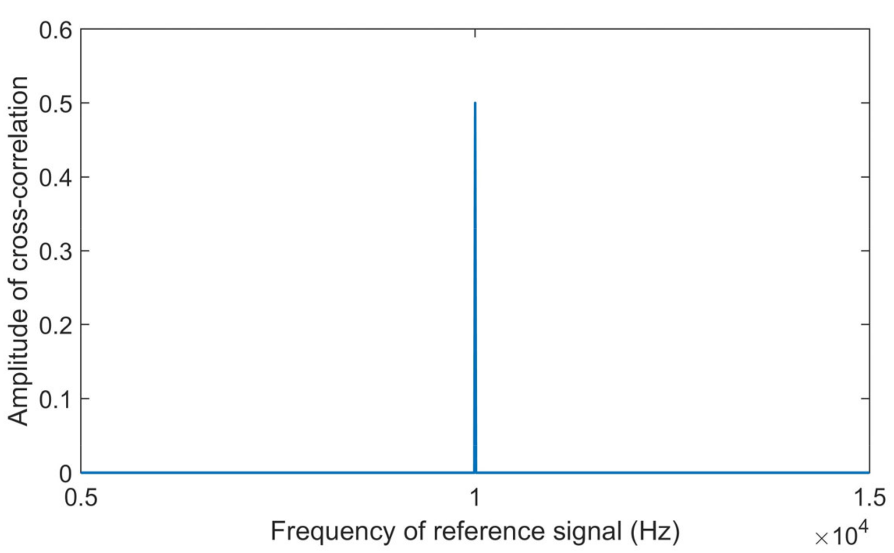
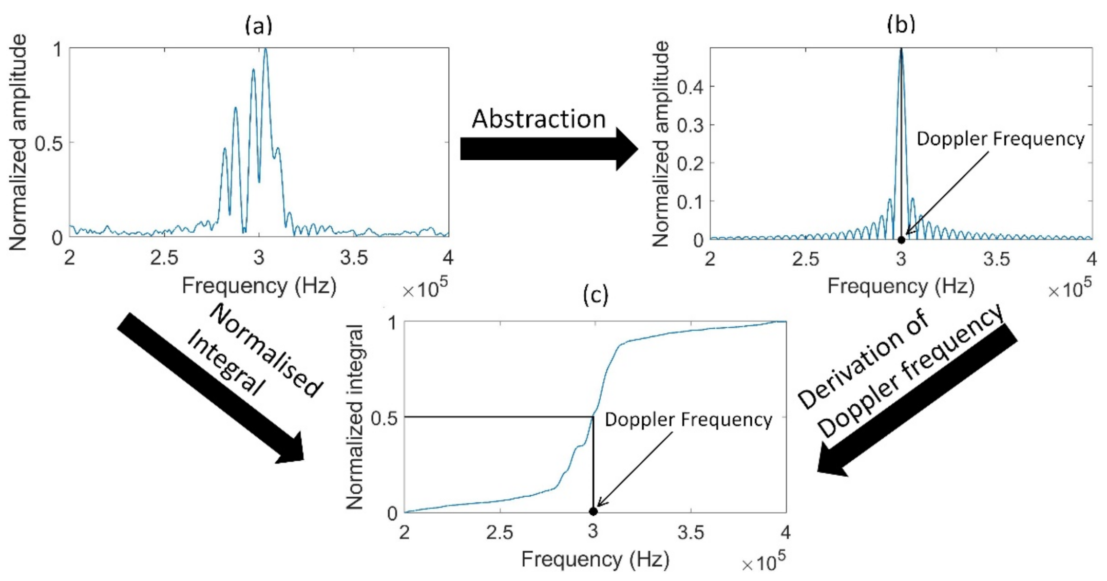
2.2. Cross-Correlation Spectrum
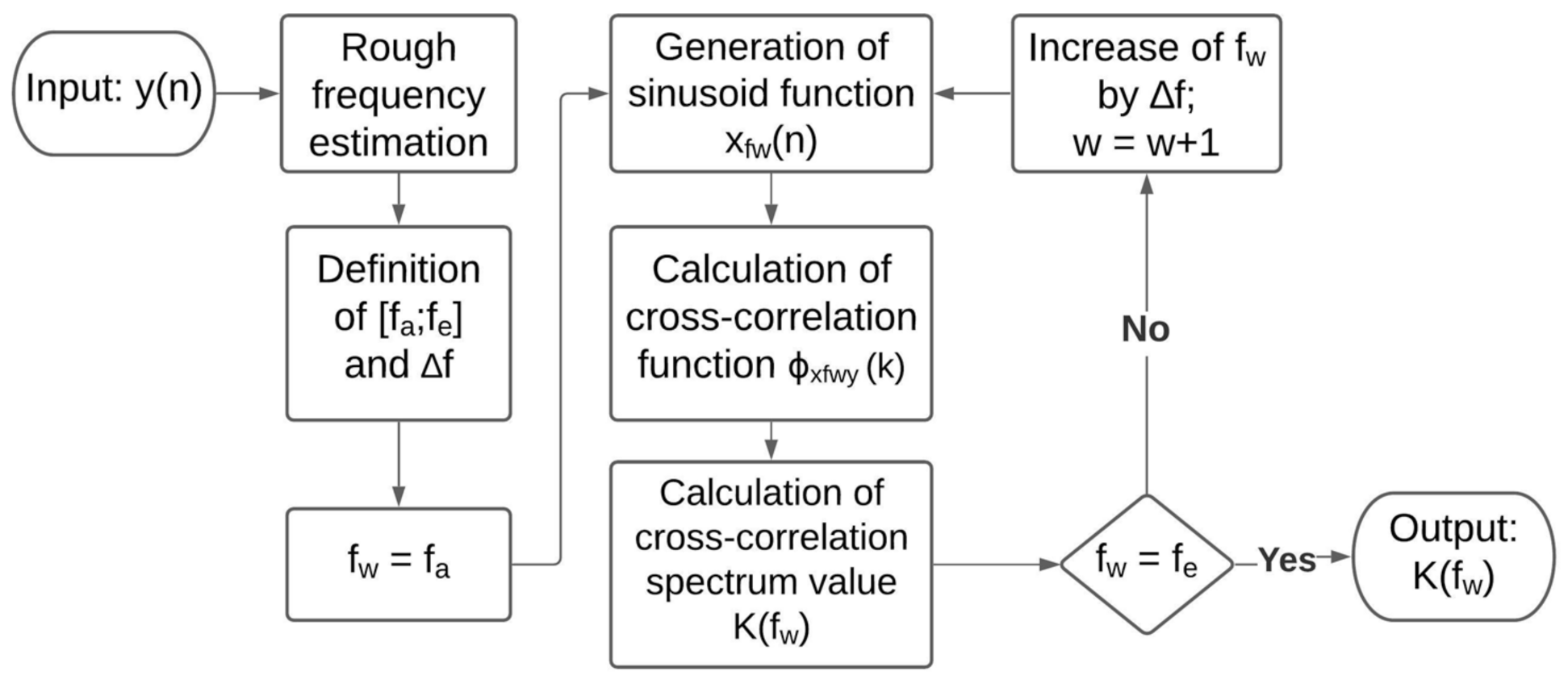
- The viewed frequency range and the frequency resolution are defined by the user. To analyze the test signal’s frequency efficiently, a rough frequency estimation is performed beforehand, to set the frequency range in a way that it is minimized as much as possible, while ensuring that the signal’s frequencies are included in the defined range. is set according to the accuracy requirements. If, for example, the signal’s frequencies are around 1 kHz and an accuracy of 0.5% is required, should be set to 1 Hz at most;
- is initialized to ;
- The sinusoid function is generated according to Equation (13);
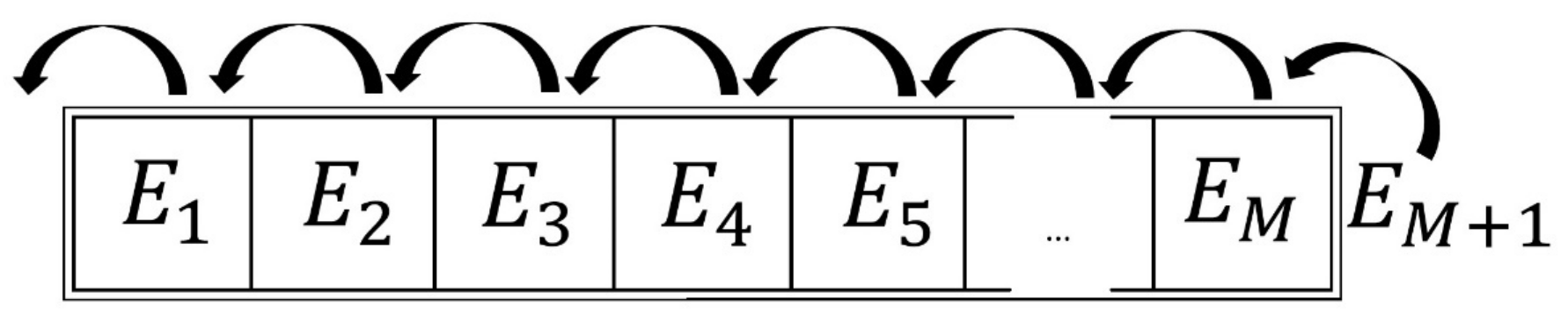
- The cross-correlation function between the test signal and is calculated using Equation (16). The parameter Z (see Equation (16)) should be set to the signal period length of ;
- The cross-correlation spectrum’s value for the current frequency is determined by identifying the amplitude of the cross-correlation function . Here, it is accomplished by finding the function’s maximum value;
- The frequency is increased by , i.e., (see Equation (14));
- The steps from 3–6 are repeated, until has been determined.
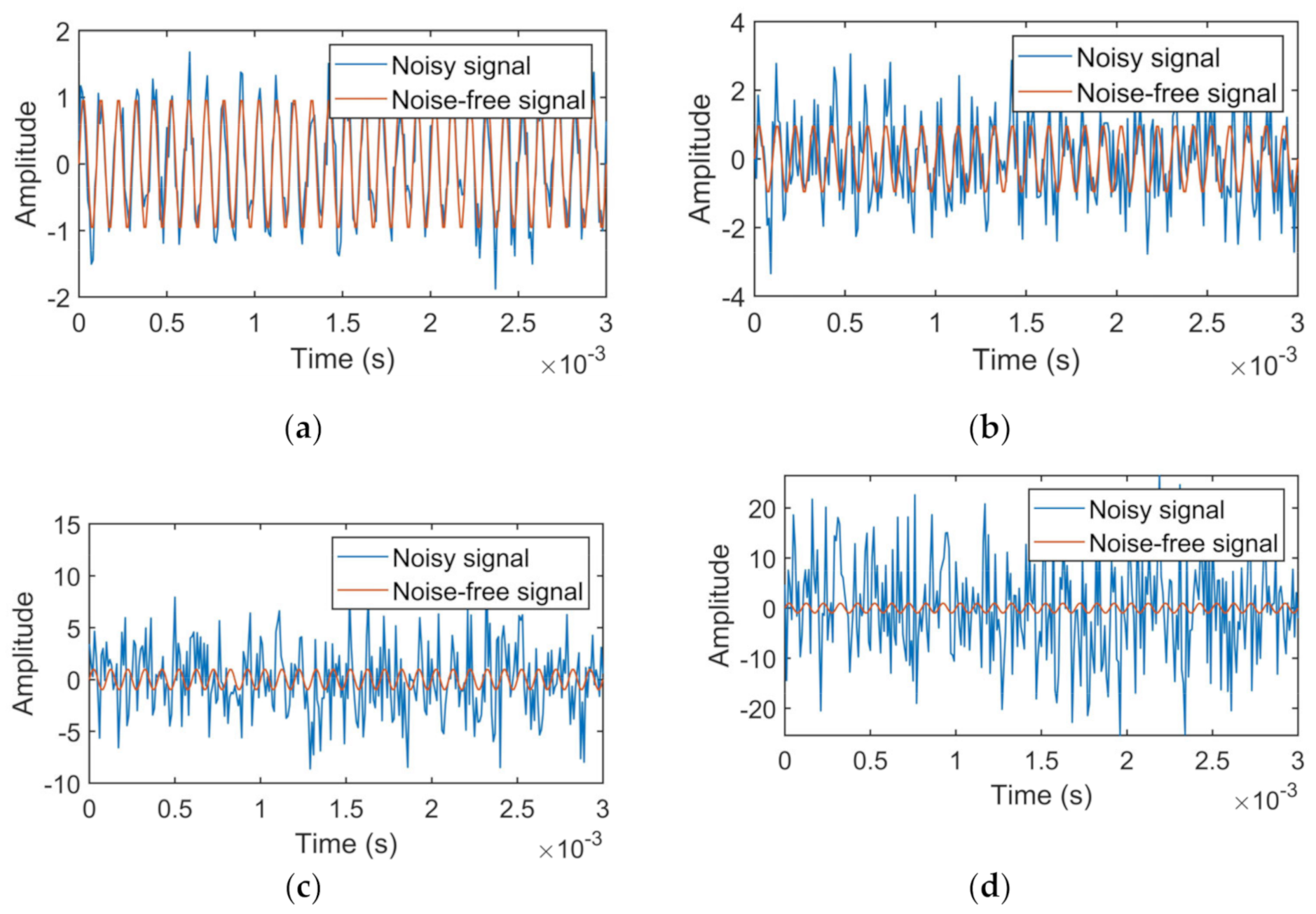
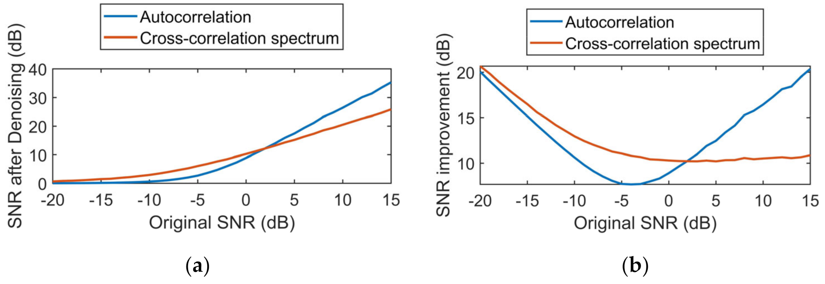
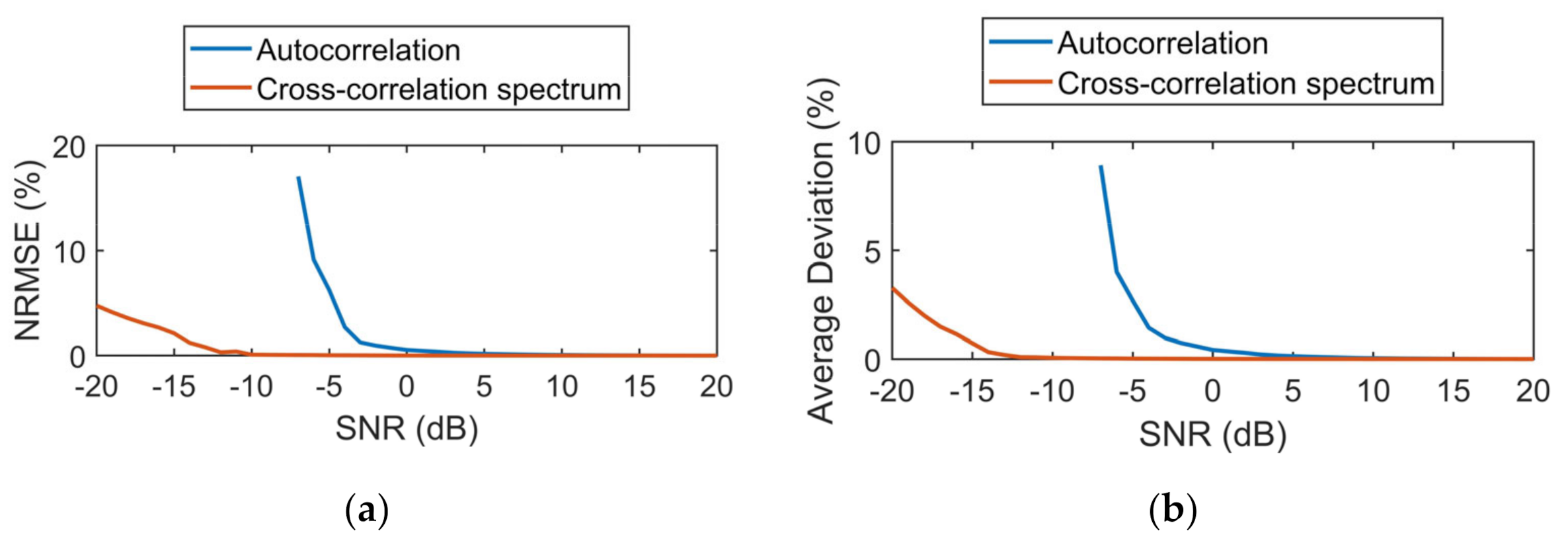
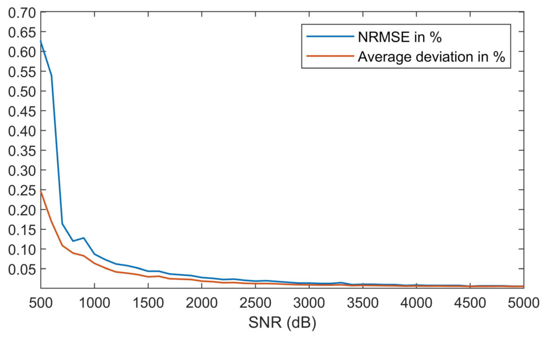
3. Simulations
4. Application Example
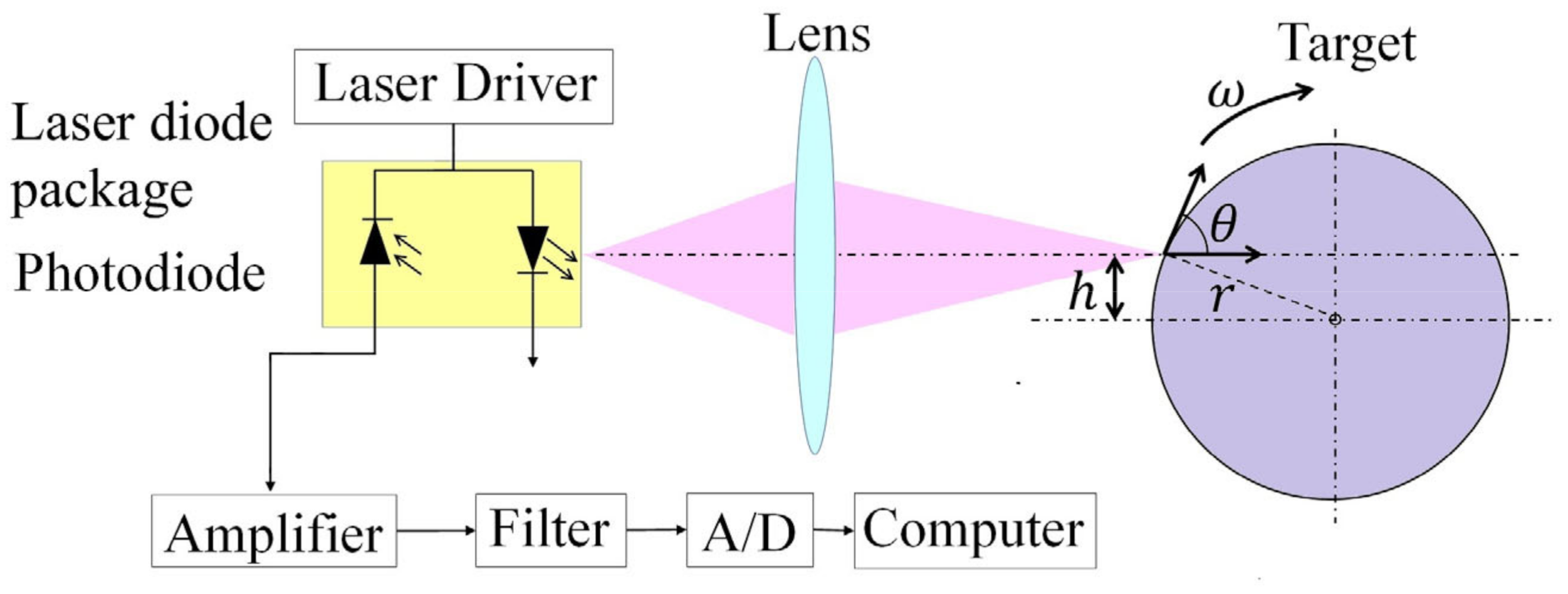
4.1. Self-Mixing Interferometry
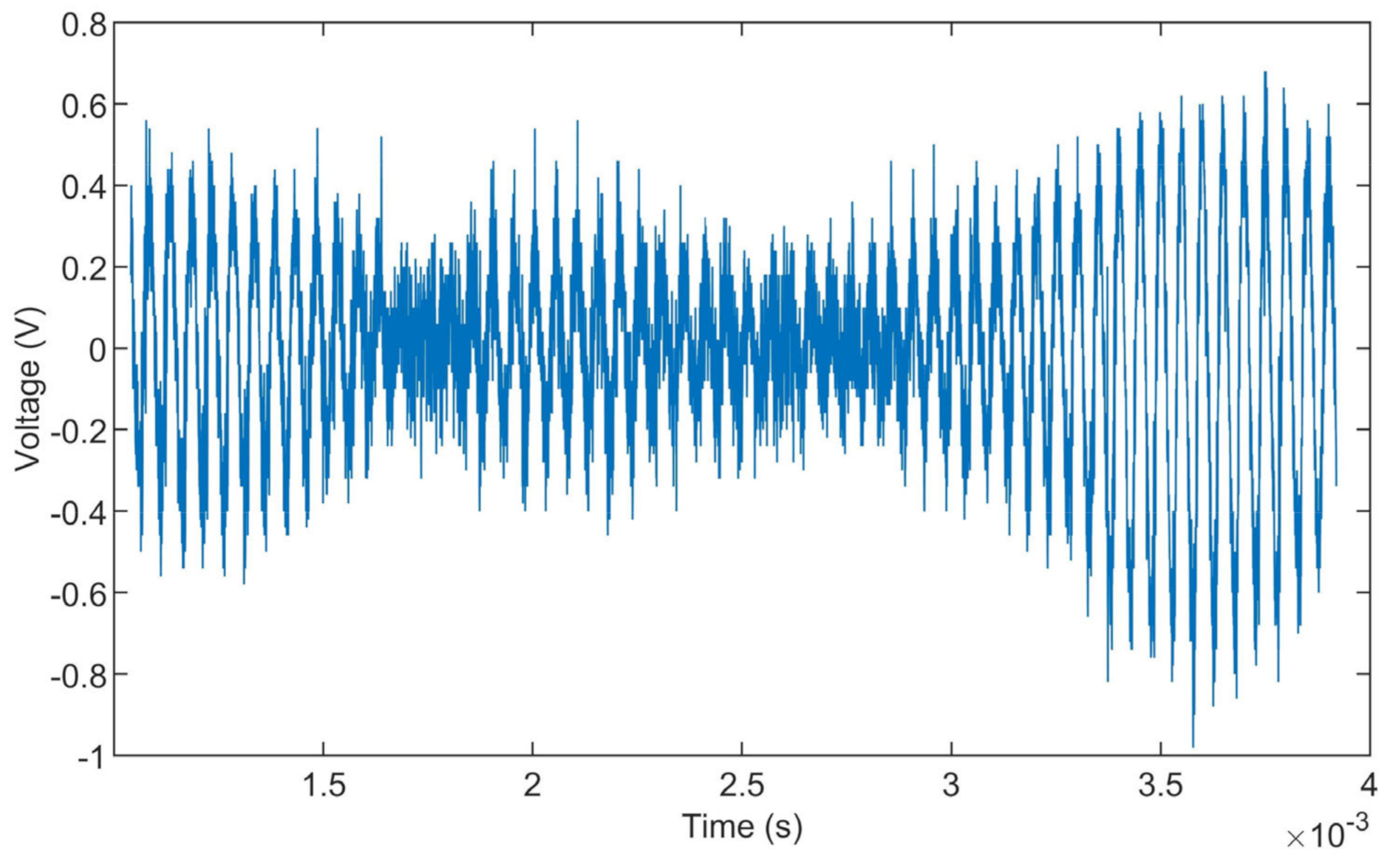
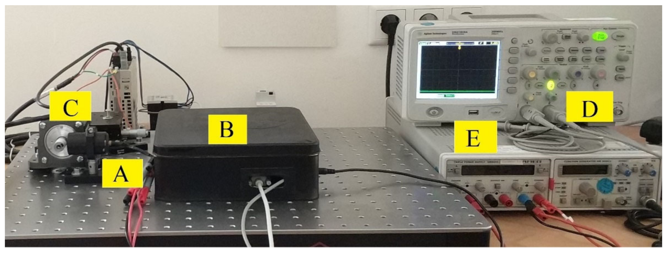
4.2. Experiments on SMI-Signals
5. Discussions
Author Contributions
Funding
Data Availability Statement
Conflicts of Interest
References
- Sanchez-Lopez, J.D.; Murrieta-Rico, F.N.; Petranovskii, V.; García, J.A.; Yocupicio-Gaxiola, R.I.; Sergiyenko, O.; Tyrsa, V.; Nieto-Hipolito, J.I.; Vazquez-Brise, M. Effect of phase in fast frequency measurements for sensors embedded in robotic systems. Int. J. Adv. Robot. Syst. 2019, 16, 1–7. [Google Scholar] [CrossRef]
- Murrieta-Rico, F.N.; Petranovskii, V.; Dalván, D.H.; Sergiyenko, O.; Antúnez-García, J.; Yocupicio-Gaxiola, R.I.; Sanchez-Lopez, J.d.D. Phase effect in frequency measurements of a quartz crystal using the pulse coincidence principle. In Proceedings of the 2020 IEEE 29th International Symposium on Industrial Electronics, Delft, The Netherlands, 17–19 June 2020; pp. 185–190. [Google Scholar]
- Liu, H.; Pang, G.K.H. Accelerometer for mobile robot positioning. IEEE Trans. Ind. Appl. 2001, 37, 812–819. [Google Scholar] [CrossRef]
- Deng, W.; Yang, T.; Jin, L.; Yan, C.; Huang, H.; Chu, X.; Wang, Z.; Xiong, D.; Tian, G.; Gao, Y.; et al. Cowpea-structured PVDF/ZnO nanofibers based flexible self-powered piezoelectric bending motion sensor towards remote control of gestures. Nano Energy 2019, 55, 516–525. [Google Scholar] [CrossRef]
- Ju, F.; Wang, Y.; Zhang, Z.; Wang, Y.; Yun, Y.; Guo, H.; Chen, B. Miniature piezoelectric spiral tactile sensor for tissue hardness palpation with catheter robot in minimally invasive surgery. Smart Mater. Struct. 2019, 28. [Google Scholar] [CrossRef]
- Karns, A.M. Development of a laser doppler velocimetry system for supersonic jet turbulence measurements. Master’s Thesis, The Pennsylvania State University, Pennsylvania, University Park, PA, USA, August 2014. [Google Scholar]
- Sun, H.; Liu, J.G.; Zhang, Q.; Kennel, R.M. Self-mixing interferometry for rotational speed measurement of servo drives. Appl. Opt. 2016, 55, 236–241. [Google Scholar] [CrossRef] [PubMed]
- Sondkar, S.Y.; Dudhane, S.; Abhyankar, H.K. Frequency measurement methods by signal processing techniques. Procedia Eng. 2012, 38, 2590–2594. [Google Scholar] [CrossRef]
- Tan, C.; Yue, Z.M.; Wang, J.C. Frequency measurement approach based on linear model for increasing low SNR sinusoidal signal frequency measurement precision. IET Sci. Meas. Technol. 2019, 13, 1268–1276. [Google Scholar] [CrossRef]
- Najmi, A.H.; Sadowsky, J. The continuous wavelet transform and variable resolution time-frequency analysis. Johns Hopkins Apl Tech. Dig. 1997, 18, 134–139. [Google Scholar]
- Khan, N.A.; Jafri, M.N.; Qazi, S.A. Improved resolution short time Fourier transform. In Proceedings of the 7th International Conference on Emerging Technologies, Islamabad, Pakistan, 5–6 September 2011; pp. 1–3. [Google Scholar]
- Liu, Y.; Jiang, Z.; Wang, G.; Xiang, J. Synchrosqueezing transform based general linear chirplet transform of instantaneous rotational frequency estimation for rotating machines with speed variation. In Proceedings of the 2020 Asia-Pacific International Symposium on Advanced Reliability and Maintenance Modeling (APARM), Vancouver, BC, Canada, 20–23 August 2020; pp. 1–5. [Google Scholar]
- Liu, J.G. Eigenkalibrierende Meßverfahren und deren Anwendungen bei den Messungen elektrischer Größen. VDI Verlag GmbH: Düsseldorf, Germany, 2000. [Google Scholar]
- Lee, Y.; Cheatham, T.P.; Wiesner, J. The application of correlation functions in the detection of small signals in noise. Available online: https://dspace.mit.edu/bitstream/handle/1721.1/4912/RLE-TR-141-04718321.pdf?sequence=1 (accessed on 28 August 2020).
- Larsen, J. Correlation Functions and Power Spectra. Available online: http://bme.elektro.dtu.dk/31610/notes/power.spectra.correlation.func.pdf (accessed on 16 September 2020).
- Wang, H.; Ruan, Y.; Yu, Y.; Guo, Q.; Xi, J.; Tong, J. A new algorithm for displacement measurement using self-mixing interferometry with modulated injection current. IEEE Access 2020, 8, 123253–123261. [Google Scholar] [CrossRef]
- Sun, H. Optimization of Velocity and Displacement Measurement with Optical Encoder and Laser Self-Mixing Interferometry. Available online: https://mediatum.ub.tum.de/doc/1507276/1507276.pdf (accessed on 14 January 2021).
- Liu, Y.; Liu, J.; Kennel, R. Rotational speed measurement using self-mixing interferometry. Appl. Opt. 2021, 60, 5074–5080. [Google Scholar] [CrossRef]
- Sun, H.; Liu, J.G.; Kennel, R.M. Improving the accuracy of laser self-mixing interferometry for velocity measurement. In Proceedings of the 2017 IEEE International Instrumentation and Measurement Technology Conference (I2MTC), Turin, Italy, 22–25 May 2017; pp. 236–241. [Google Scholar]
- Kliese, R.; Rakić, A.D. Spectral broadening caused by dynamic speckle in self-mixing velocimetry sensors. Opt. Express 2012, 20, 18757–18771. [Google Scholar] [CrossRef] [PubMed]
- Mowla, A.; Nikolic, M.; Taimre, T.; Tucker, J.; Lim, Y.; Bertling, K.; Rakic, A. Effect of the optical system on the Doppler spectrum in laser-feedback interferometry. Appl. Opt. 2015, 54, 18–26. [Google Scholar] [CrossRef] [PubMed]


| Scheme | NRMSE in % | Average Deviation in % |
|---|---|---|
| −20 | 4.7141 | 3.2802 |
| −15 | 2.1118 | 0.7325 |
| −10 | 0.0885 | 0.0652 |
| −5 | 0.0382 | 0.0262 |
| −4 | 0.0355 | 0.0244 |
| −3 | 0.0312 | 0.0214 |
| −2 | 0.0240 | 0.0182 |
| −1 | 0.0191 | 0.0154 |
| 0 | 0.0145 | 0.0140 |
| 1 | 0.0136 | 0.0135 |
| 2 | 0.0125 | 0.0124 |
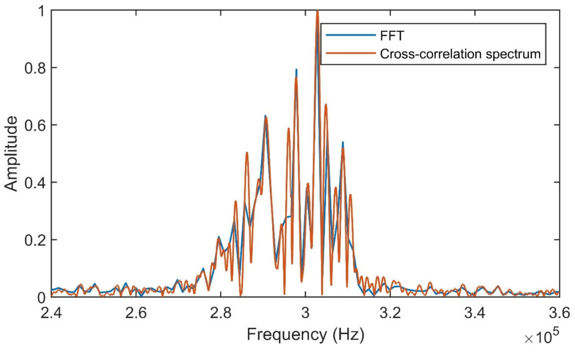
| FFT | Cross-Correlation Spectrum | ||
|---|---|---|---|
| Frequency | Energy | Frequency | Energy |
| 301,513 | 0.1750 | … | |
| 301,480 | 0.1600 | ||
| 301,490 | 0.1618 | ||
| 301,500 | 0.1643 | ||
| 301,510 | 0.1665 | ||
| 301,520 | 0.1695 | ||
| 301,530 | 0.1727 | ||
| 301,540 | 0.1765 | ||
| 301,550 | 0.1803 | ||
| 301,560 | 0.1841 | ||
| 302,734 | 1 | … | |
| 302,710 | 0.9808 | ||
| 302,720 | 0.9827 | ||
| 302,730 | 0.9840 | ||
| 302,740 | 0.9861 | ||
| 302,750 | 0.9894 | ||
| … | |||
| 302,820 | 0.9986 | ||
| 302,830 | 0.9996 | ||
| 302,840 | 1 | ||
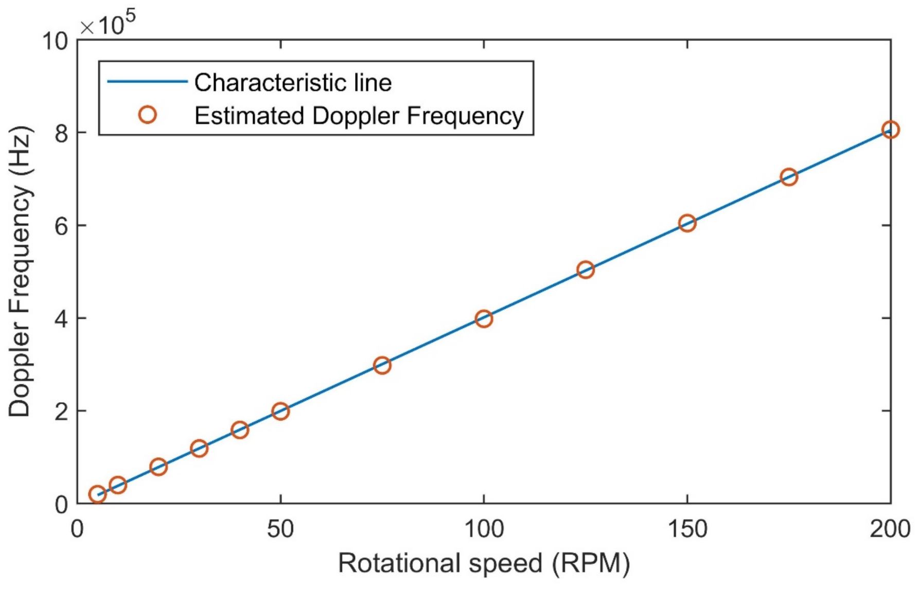
| Rotational Speed | Doppler Frequency in Hz | Doppler Frequency of the Characteristic Line in Hz | Linearity |
|---|---|---|---|
| 5 | 19,863.79 | 17,920.50 | −0.24% |
| 10 | 39,692.23 | 38,101.50 | −0.20% |
| 20 | 78,921.36 | 78,463.50 | −0.06% |
| 30 | 118,590.4 | 118,825.5 | 0.03% |
| 40 | 158,504.6 | 159,187.5 | 0.09% |
| 50 | 198,683.8 | 199,549.5 | 0.11% |
| 75 | 297,685.6 | 300,454.5 | 0.35% |
| 100 | 398,130.6 | 401,359.5 | 0.40% |
| 125 | 503,959.1 | 502,264.5 | −0.21% |
| 150 | 604,433.3 | 603,169.5 | −0.16% |
| 175 | 703,830.3 | 704,074.5 | 0.03% |
| 200 | 806,050.0 | 804,896.9 | -0.12% |
Publisher’s Note: MDPI stays neutral with regard to jurisdictional claims in published maps and institutional affiliations. |
© 2021 by the authors. Licensee MDPI, Basel, Switzerland. This article is an open access article distributed under the terms and conditions of the Creative Commons Attribution (CC BY) license (https://creativecommons.org/licenses/by/4.0/).
Share and Cite
Liu, Y.; Liu, J.; Kennel, R. Frequency Measurement Method of Signals with Low Signal-to-Noise-Ratio Using Cross-Correlation. Machines 2021, 9, 123. https://doi.org/10.3390/machines9060123
Liu Y, Liu J, Kennel R. Frequency Measurement Method of Signals with Low Signal-to-Noise-Ratio Using Cross-Correlation. Machines. 2021; 9(6):123. https://doi.org/10.3390/machines9060123
Chicago/Turabian StyleLiu, Yang, Jigou Liu, and Ralph Kennel. 2021. "Frequency Measurement Method of Signals with Low Signal-to-Noise-Ratio Using Cross-Correlation" Machines 9, no. 6: 123. https://doi.org/10.3390/machines9060123
APA StyleLiu, Y., Liu, J., & Kennel, R. (2021). Frequency Measurement Method of Signals with Low Signal-to-Noise-Ratio Using Cross-Correlation. Machines, 9(6), 123. https://doi.org/10.3390/machines9060123