Article

Adjustable Speed Control and Damping Analysis of Torsional Vibrations in VSD Compressor Systems

by
Mattia Rossi
,
Maria Stefania Carmeli
and
Marco Mauri
*,†
Department of Mechanics, Politecnico di Milano, Via La Masa 1, 20156 Milano, Italy
*
Author to whom correspondence should be addressed.
These authors contributed equally to this work.
Machines 2021, 9(12), 374; https://doi.org/10.3390/machines9120374
Submission received: 23 November 2021 / Revised: 13 December 2021 / Accepted: 15 December 2021 / Published: 20 December 2021
(This article belongs to the Section Electrical Machines and Drives)

Abstract

:
This paper proposes a model-based two-degree-of-freedom (2DOF) speed control for a medium voltage (MV) variable speed drive (VSD) connected to a centrifugal compressor (CC) train. Torsional mode excitations in the drive shaft due to converter switching behaviour are considered. An effective description of the harmonics transfer is proposed. The tuning strategy aims to optimize the tracking behaviour of the step and ramp command, taking care of critical speed excitations. The stability of the closed-loop dynamics against time delay and drive parameter variations are studied by means of Nyquist diagrams and time-domain simulations. A descriptive method for the process damping behaviour is proposed. The control strategy is evaluated through simulations as well as an experimental setup, based on a hardware in the loop (HIL) in a master–slave configuration.

1. Introduction

In the oil and gas industry, voltage source drives (VSDs) are key elements from liquefied natural gas trains to subsea scenarios [1], because they adjust their speed according to the centrifugal compressor (CC) train requirements, maximizing overall efficiency and making them suitable as prime movers [2,3]. However, there may be harmful interactions in the coupling shaft, such as torsional mode excitations and fatigue cycles. The intrinsic nature of switching-based drives produces a pulsating torque transfer on the transmission components that can match some torsional natural frequencies (TNFs), implying an oscillating behavior of the state variables [4,5]. In fact, crack and/or lifetime reduction can happen if the torque constraints are not satisfied [6]. Hence, resonant mechanical models, such as a dual-inertia elastic systems, are commonly used to design a control law [7,8,9].
Looking to the industrial feasibility of a digital signal processor (DSP), this paper proposes a 2DOF controller, based on classical PI cascade control architecture, with the aim to obtain good reference tracking and load torque rejection for each DOF. We additionally aim to achieve a MV-VSD that follows a CC speed-profile in the presence of TNFs excitation. The selection of this control architecture is due to the necessity of implementing this control on existing industrial controllers without changing the implemented control strategy. Model-based pole placement rules are used to design the feedback controller, and aimed to reject the load torque changes. A feedforward action that optimizes the speed tracking is properly selected according to the actual reference profile, avoiding excessive coupling torque vibrations. More advance controls or estimators [10] could be used to improve the control performances, but these implementations are out of the scope of this paper.
Usually, a CC profile involves dynamic ramp references with different slopes (e.g., the pressure cycle does not vary instantaneously), and more than only a step-command of the load torque (e.g., valve opening, starting another CC in parallel) [11]. Hence, the case-study analysed in the paper considers a mixed-speed profile and a quadratic load torque, both coming from a high-level CC pressure map.
The paper also proposes a damping analysis, because a closed-loop strategy indirectly affects the process damping ζP at each TNF, influencing the superimposition of the mechanical damping ζmech and the electrical damping ζelet. Delayed control algorithm may increase/sustain potential failure conditions [12,13]. Thus, a descriptive approach to consider the time delay influence onto ζP is given. The simulated control strategy is then experimentally validated through a hardware-in-the-loop (HIL) in a master–slave configuration. The outline of the paper is as follows. A description of the case study requirements and the related mechanical modeling are given in Section 2 and Section 3. Section 4 presents the AC-DC-AC stage and the harmonics transfer, followed by the combined control design in Section 5 and Section 6. Section 7 addresses robustness issues and process damping description. In Section 8, the control design is compared and verified by means of HIL test.

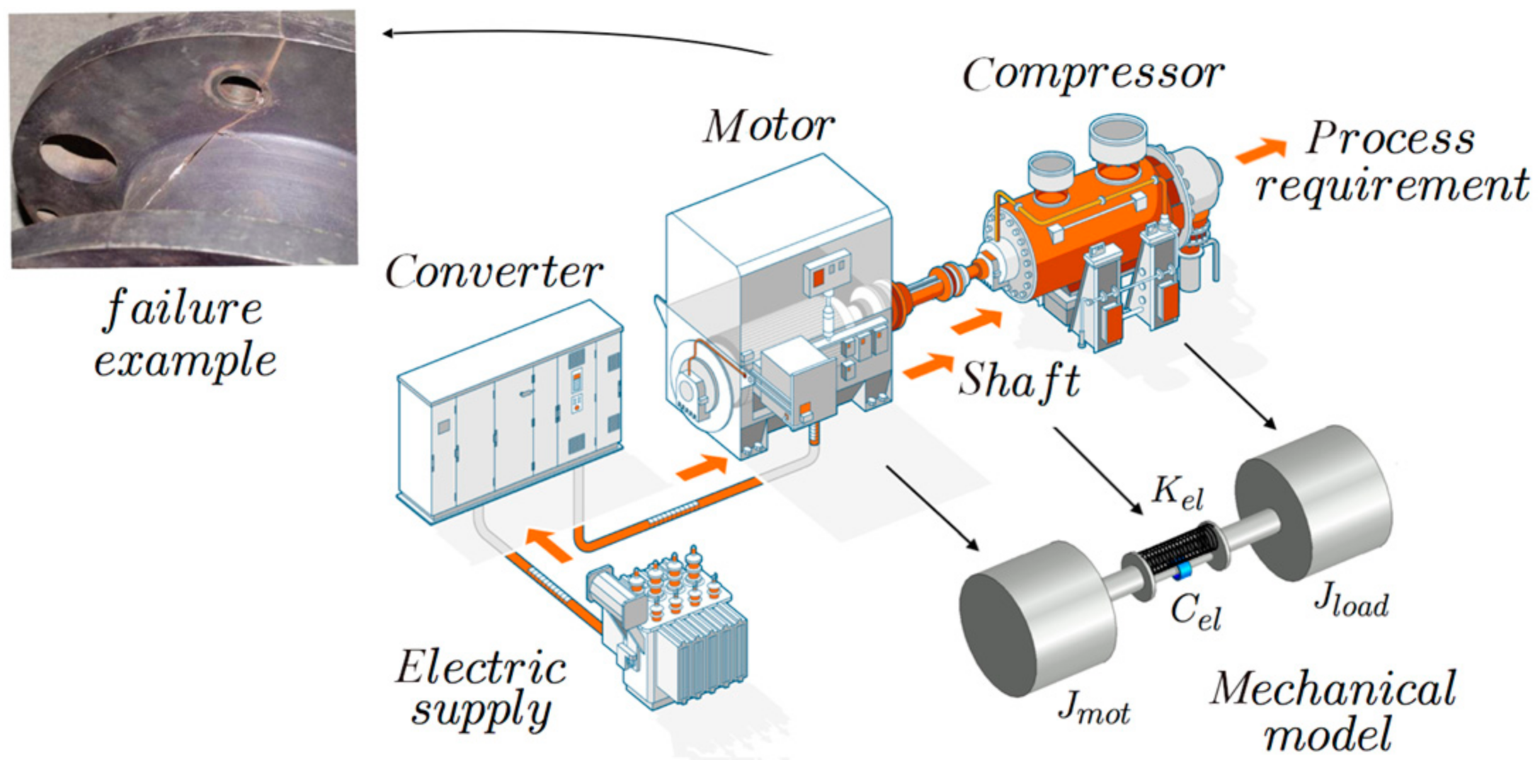
2. MV Field Case Application

This paper presents a case study of an 8 MW industrial application, which consists of a VSD directly connected to a CC train through a coupling shaft. For reasons of simplicity, this paper considers the CC as the only load stage. The VSD is based on an induction motor and a multilevel conversion unit, which comprises an Active Neutral Point Clamped 5-level (5-level ANPC) Voltage Source Inverter (VSI) driven by a 36-pulse diode-bridge rectifier. The VSD control system has to guarantee the command tracking of the CC speed profile, which implies a certain pressure injection from the load stage to the next (outer pressure/volume controls). A complete scheme is shown in Figure 1, while the parameters are given in Table 1.
Let us consider for this analysis that the system should follow the speed profile shown in Figure 2. Two steady-state values are considered for testing purpose: 10% and 20% of the rated speed Ωrat. Furthermore, let us assume a non-linear load torque characteristic m l o a d t affecting the CC: it follows m l o a d t = f v Ω load 2 t + f s .
In particular, considering mload (t) as a disturbance, Figure 2 also includes a critical event given by a sudden load change, e.g., a downstream valve opening at t = 50 s.

3. Drive train Mechanical Modeling

In a MV field, the mechanical design of the drive-train provides TNFs between 0–100 Hz; such range mainly includes the first TNF and second TNF, see [3,10]. This paper focuses on a dual-inertia model, which correctly describes the first torsional mode associated to the first TNF.
J m d Ω m o t d t = m m o t m c o u p l i n g J l d Ω l o a d d t = m c o u p l i n g m l o a d m c o u p l i n g = K e l θ m o t θ l o a d + C e l ( Ω m o t Ω l o a d ) ,
The angular positions of the motor and the load are θmot, and θload, respectively. The motor torque is mmot, the load torque is mload and the coupling torque is mcoupling. The angular speeds of the motor and the load are Ωmot and Ωload, respectively. Using the model (1), the transfer function G31(s) from Ω m o t to m m o t is defined in (2):
G 31 ( s ) = G m o t ( s ) = Ω m o t m m o t = 1 J t o t N m o t ( s ) D ( s ) ,
where Jtot = Jmot + Jload and the numerator Nmot(s) and the denominator D(s) are given in (3).
N m o t ( s ) = J l o a d s 2 + C e l s + K e l D ( s ) = J m o t J l o a d J t o t s 2 + C e l s + K e l
Equation (2) can be rewritten as in (4), where the main mechanical parameters that characterize the elasticity of the drive shaft are identified: the resonance parameters ζres, ωres, and the anti-resonance parameters ζant, ωant.
G m o t ( s ) = 1 J t o t s 1 + 2 ζ a n t ω a n t s + 1 ω a n t 2 s 2 1 + 2 ζ r e s ω r e s s + 1 ω r e s 2 s 2 ω r e s = J t o t K e l J m o t J l o a d , ω a n t = K e l J l o a d ζ r e s = C e l 2 J t o t J m o t J l o a d K e l , ζ a n t = C e l 2 1 J l o a d K e l
In (4), ωres is associated with the poles of the denominator and ζres is the damping coefficient; ωant is associated to the zero of numerator and ζant is the damping coefficient.
These two eigenvalues for the system under analysis define the anti-resonance frequency at ωant = 2π6.6 rad/s, ζant = 4.3 × 10⁻⁴ and the first Torsional Natural Frequency at ωres = 2π17 rad/s, ζres = 1.1 × 10⁻³. The first torsional mode associated with the first TNF at ωres is shown in a 3D plot in Figure 3.

4. Analysis of the VSD Vibrating Behavior

Although the motor drive pulsating torque is the main source of TNFs excitation, the vibration behaviour in terms of amplitude and oscillation decay is related to the VSD integration in the closed-loop control strategy. A complete analysis of the torsional response needs to study:
  • The AC-DC-AC topology and the torque spectrum;
  • The control loops design and the oscillation characteristics.
An electrical scheme overview of the motor drive is shown in Figure 4. As discussed in [4,11], the AC-DC-AC stage produces integer harmonics and interharmonics in torque (referred to DC-link coupling). The overall excitation content transferred to the shaft line is computed in (5), as a function of the motor speed and supply frequency. m, k are integer multipliers according to the following cases:
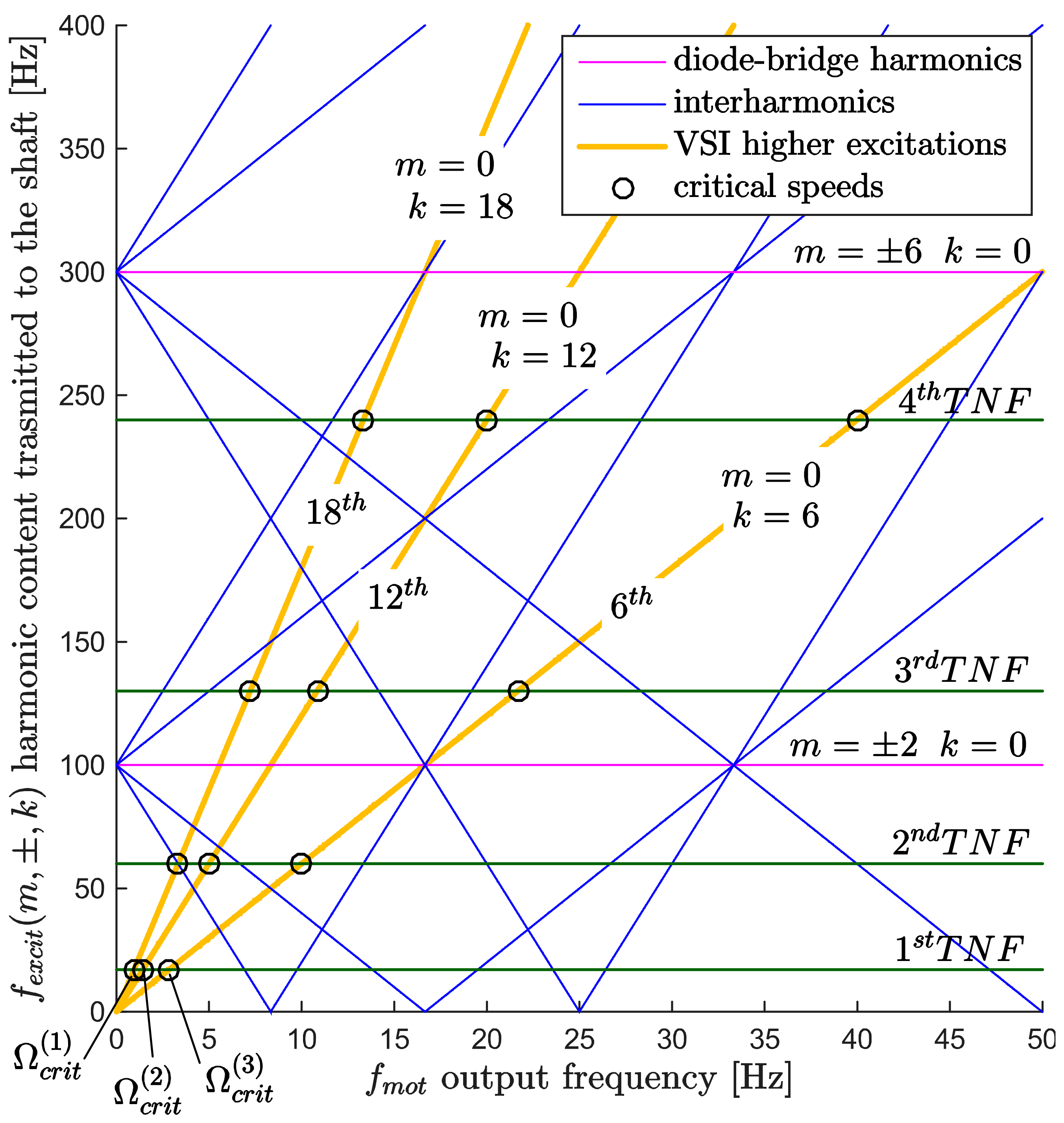
  • m = 0 and k ≠ 0 → VSI inverter integer harmonic;
  • m ≠ 0 and k = 0 → diode-bridge integer harmonic;
  • m ≠ 0 and k ≠ 0 → interharmonics DC-link.
f e x c i t ( m , ± k ) = m f l i n e ± k f m o t ,
where fmot = nppΩmot/60. Experimentally, the motor torque running the VSD at the rated speed Ωrat in no-load condition leads to a motor torque as in Figure 5. Performing a spectrum analysis of the air-gap torque pulsations, the highest excitations components nk are the sixth, twelfth, and eighteenth, with a torque magnitude close to the 2% of the rated torque; the other components have a negligible magnitude. Hence, the pulsating torque is mainly defined by the VSI switching behaviour, kfmot with k = 6, 12, 18.

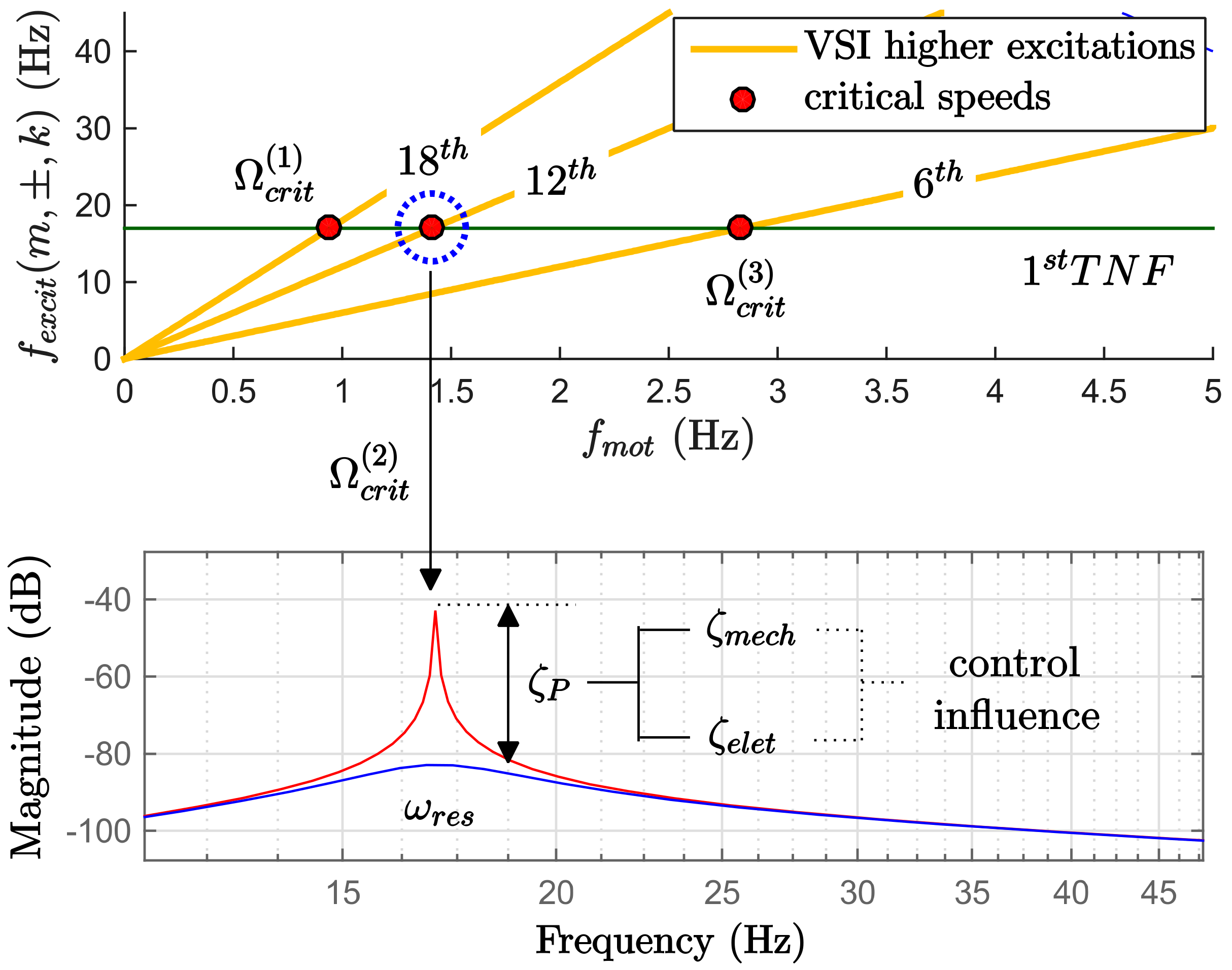
5. Campbell Diagram and First Analysis

The torsional behaviour, the torque content and the application speed range information can be merged in a Campbell diagram: a 2D graphical representation shown in Figure 6. The intersection points between the TNF horizontal line and the excitations lines transferred to the shaft fexcit (m, ±, k) identify the critical speeds Ω(i)crit. They can be computed for the first TNF, as in (6).
Ω c r i t ( i ) = ω r e s 2 π f l i n e n k ( i = 1 , 2 , 3 ) ,
According to Table 2, Ωcrit(1), Ωcrit(2), Ωcrit(3), are excited at quite low speeds: this can be a problem either during a start-up or for a speed reference in their neighborhood.
Furthermore, due to the VSD closed-loop integration, the actual damping factor at each Ω(i)crit is a combination of the mechanical one given by the shaft proprieties ζmech and the electrical damping ζelet mainly given by the electrical motor damping ζmot [14]. The control strategy defines the contributions of each term, and it is possible to analyze this effect with a more general definition of an overall process damping coefficient ζP, as shown in Figure 7 and given in (7).
ζ P = f ζ m e c h , ζ e l e t ζ m e c h = ζ r e s ζ e l e t = f ζ m o t ,
One way to describe this coefficient is through the closed-loop transfer function of the process, where the control architecture adds additional dynamics besides Gmot(s) (4).
For the speed control a 2DOF piece of architecture that includes a feedback controller R(s) aimed to improve the load torque rejection, a feedforward controller C(s) aimed to optimize the command-tracking performance [7,15] has been selected.
A full scheme is reported in Figure 8. The load speed Ωload is controlled by closing the feedback loop on the motor speed Ω ^ m o t that came out from an estimator E(s), seen as an intermediate stage between Ωmot and Ω ^ m o t , Gload(s) is described through Gmot and G41 = Ωload/mmot, as given in (8).
G l o a d ( s ) = Ω l o a d Ω m o t = G 41 ( s ) G m o t ( s ) = N l o a d ( s ) N m o t ( s ) ,
where N l o a d s = s C e l + K e l it is possible to define a cross-coupling term G d s , as shown in (9), in order to consider the effect of the m l o a d torque on motor speed Ω m o t :
G d ( s ) = m m o t m l o a d = G 42 ( s ) G 41 ( s ) = N d ( s ) N l o a d ( s ) ,
where N d s = J m o t s 2 + s C e l + K e l .

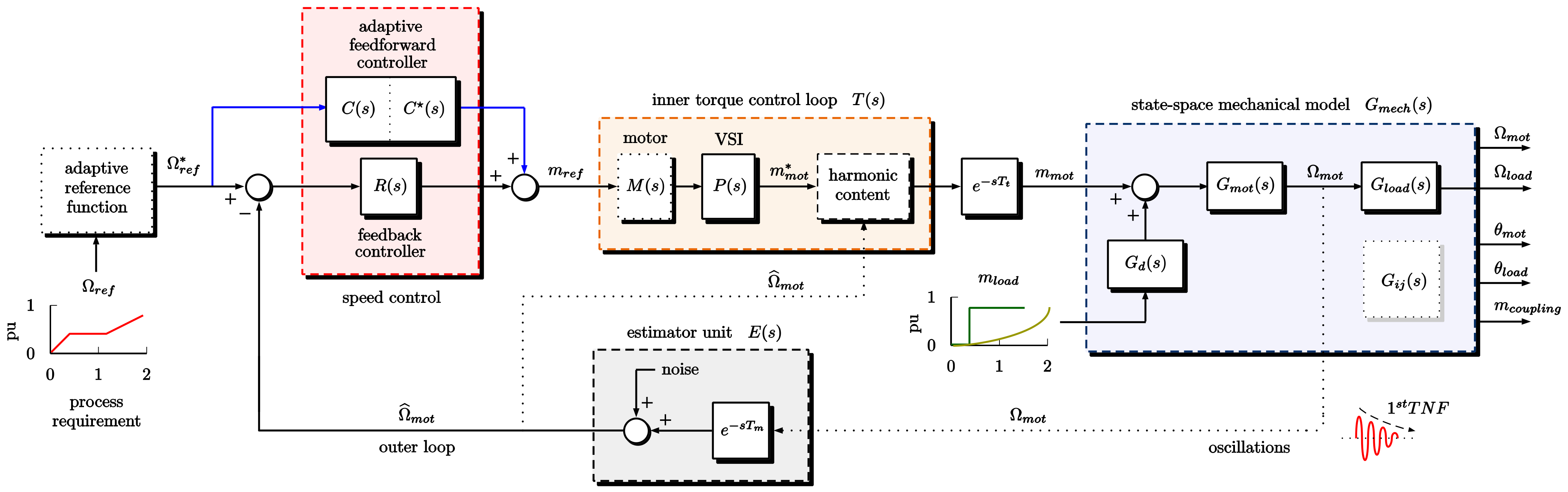
6. Torque Control Loop

The torque control loop transfer function T(s) considers a current control aimed to adjust the voltage input of a modulator that fed the VSI. A simple modeling splits T(s) into two transfer functions: the power stage P(s) and the harmonic stage H(s). Assuming a high bandwidth for the current controller, the VSI mainly influences high-frequency dynamics, then the power stage can be modeled as in (10):
P ( s ) = m m o t * m r e f = 1 1 + s T p ,
where Tp = 5 ms according to the cycle time of the switching states for the system under analysis [16,17,18,19]. Considering the spectrum analysis in Figure 5, the harmonic content of the motor torque mmot is represented through a critical speeds function H(s) as follows:
m m o t = m m o t * 1 + A n k sin n k Ω m o t t H ( s ) : m m o t m m o t * { 1 + A sin ( 6 t h Ω m o t t ) } + A sin ( 12 t h Ω m o t t ) } + A sin ( 18 t h Ω m o t t ) }
where A is the average magnitude of the harmonic components (i.e., 2% from Figure 5).

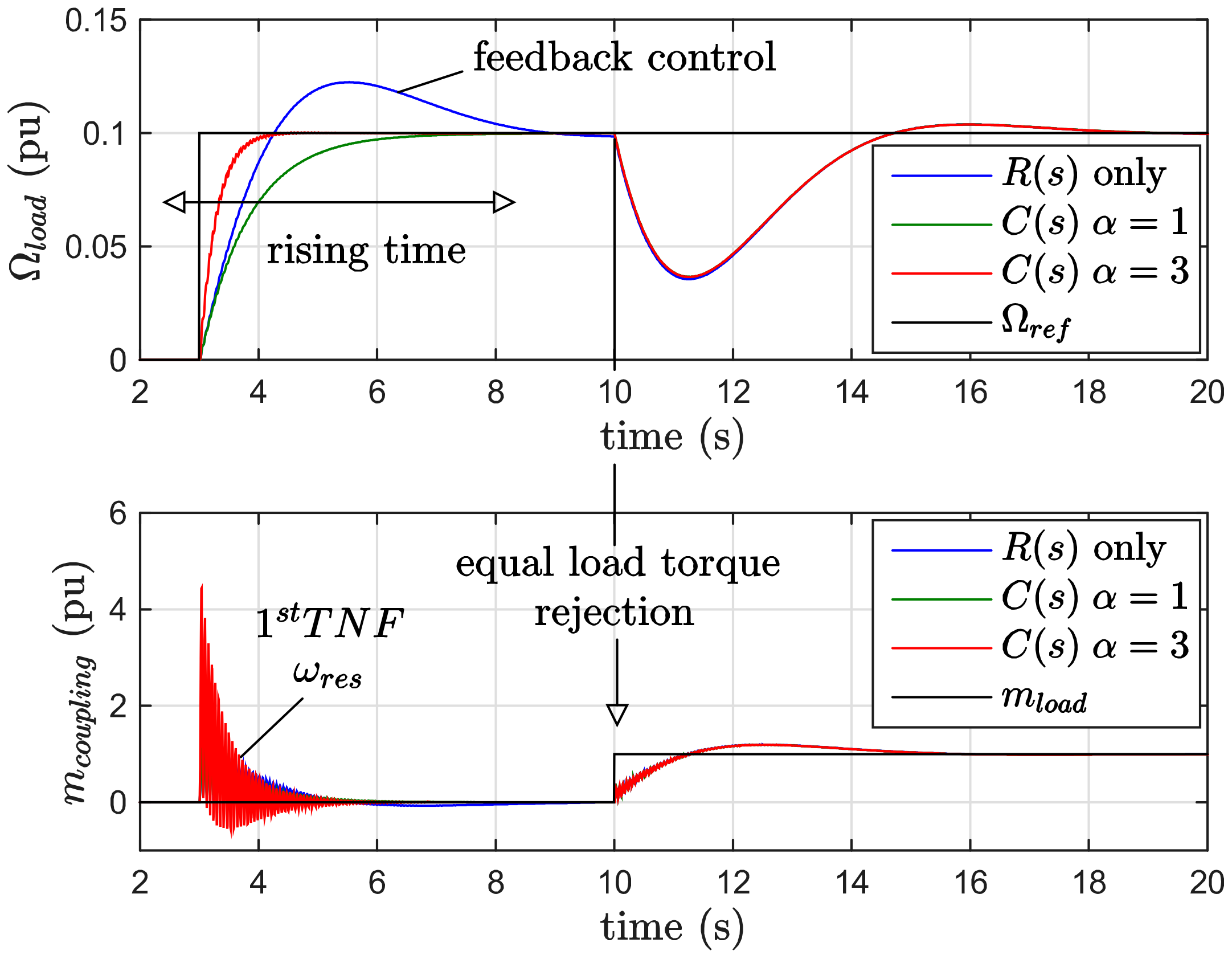
6.1. Feedback Controller Design

The control scheme architecture is shown in Figure 8. The selected PI-feedback controller is R s = k p + k i / s where kp and ki are the proportional and integral gains, respectively. Closing the feedback loop on the motor speed Ωmot, the open-loop transfer function L(s) is given by (12):
L ( s ) = R ( s ) G m o t ( s ) = ( s k p + k i ) N m o t ( s ) J t o t s 2 D ( s ) .
Hence, the command-tracking transfer function from Ωref to Ωload is F c o m ( s ) = L ( s ) / 1 + L ( s ) G l o a d ( s ) and leads to the transfer function (13):
F c o m ( s ) = Ω l o a d Ω r e f = ( s k p + k i ) N l o a d ( s ) J t o t s 2 D ( s ) + ( s k p + k i ) N m o t ( s ) .
A model-based pole placement rule is chosen as control design solution. This approach is based on the following assumptions: undamped condition (Cel = 0), ideal actuation for T(s) = 1 and E(s) = 1. In particular, (13) can be rewritten in an equivalent form such as (14):
F c o m ( s ) = k p ω 1 2 ω 2 2 k i s k p + k i s 2 + 2 ζ 1 ω 1 s + ω 1 2 s 2 + 2 ζ 2 ω 2 s + ω 2 2 p 1 , 2 a n d p 3 , 4 ,
where there are four complex closed-loop poles p1,2 and p3,4 defined by the coefficients (ω1, ζ1) and (ω2, ζ2) that are the function of the previous system parameters {Jmot, Jload, Kel} and controller parameters {kp, ki}. Comparing (12) and (13), it is possible to write the algebraic system (15):
k p = J m o t J l o a d ω 1 2 ω 2 2 K e l k i = 2 J m o t ζ 1 ω 1 + ζ 2 ω 2 0 = J m o t ω 1 2 + 4 ζ 1 ω 1 ζ 2 ω 2 + ω 2 2 K e l J t o t J l o a d k i 0 = 2 J m o t J l o a d ζ 1 ω 1 ω 2 2 + ζ 2 ω 2 ω 1 2 k p K e l .
As shown in Figure 9, to design the controller, a classical pole placement could be used assuming identical damping ζ1 = ζ2, identical real part ω1 ζ1 = ω2 ζ2 and identical radius ω1 = ω2 [15].
However, a model-based design rule can be tailored to the first known TNF dynamics [20,21]. Assuming p1,2 and p3,4 are placed into separate s-plane regions, one of them is selected as the dominant one, and then the other resonant poles are computed in order to assure enough damping. As R(s) has only two tunable parameters {kp, ki}, the poles cannot be arbitrarily placed [8], so an analytical procedure to design the controller could be:
1.
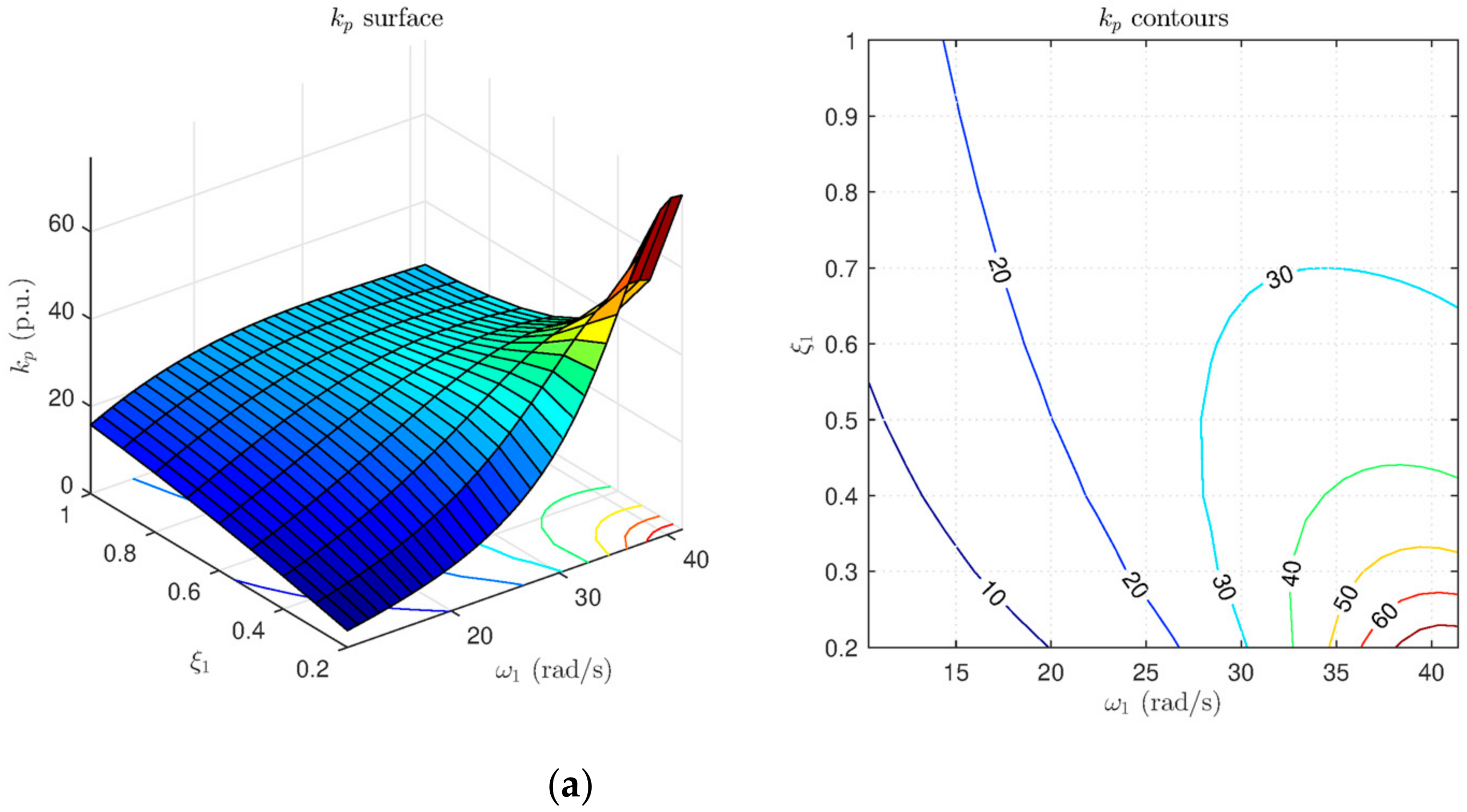
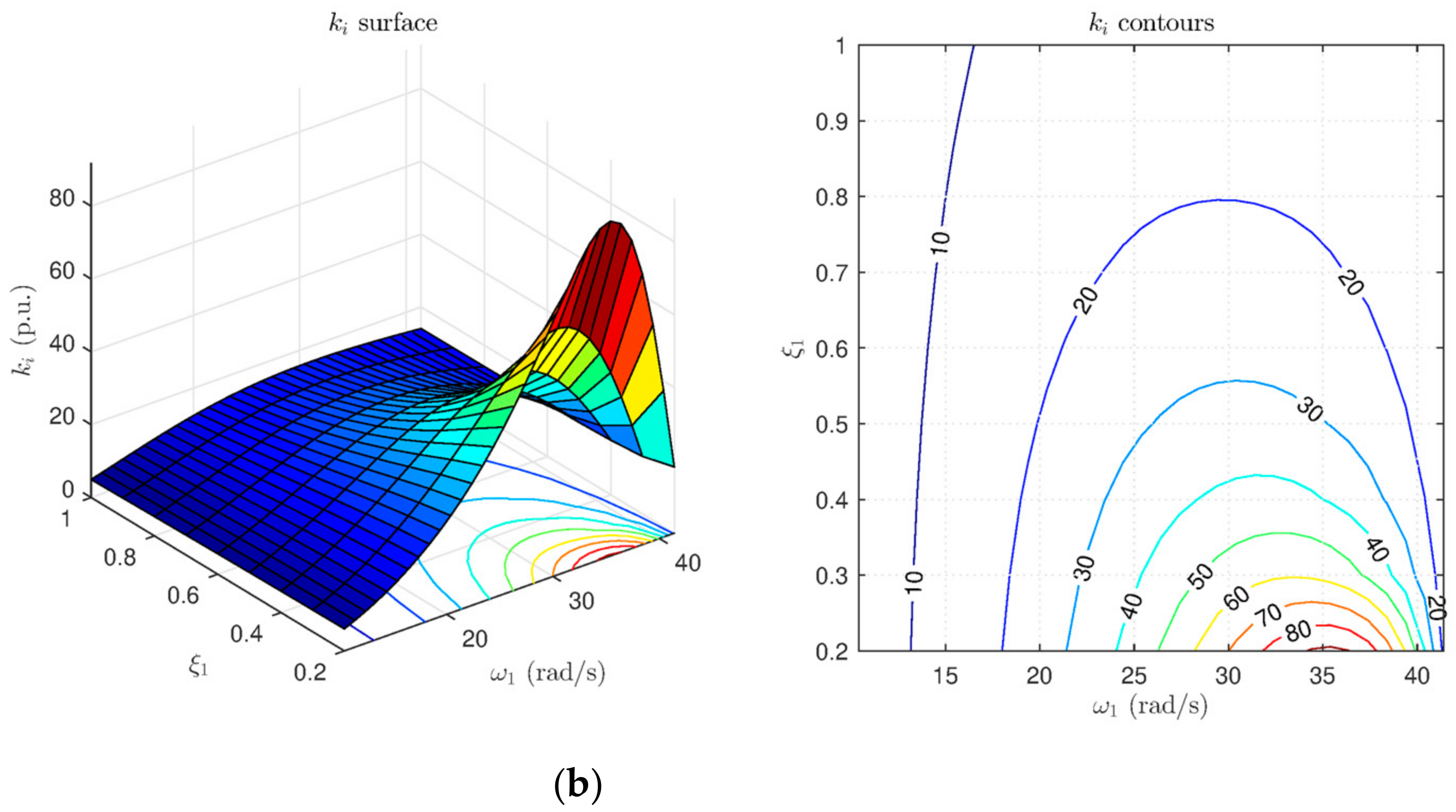
From (15), kp and ki are written as a function of the pole pair p1,2, based on {Jmot, Jload, Kel, ω1, ζ1} as in (16):
k p = 2 J m o t ζ 1 ω 1 J t o t K e l J m o t J l o a d ω 1 2 + J l o a d ω 1 2 K e l + 4 ζ 1 2 2 K e l J l o a d ω 1 2 + J l o a d ω 1 2 K e l + 4 ζ 1 2 2 k i = J m o t ω 1 2 J t o t K e l J m o t J l o a d ω 1 2 + J l o a d ω 1 2 K e l + 4 ζ 1 2 1 J t o t J m o t K e l J l o a d ω 1 2 + J l o a d ω 1 2 K e l + 4 ζ 1 2 2
Both kp and ki parameters are graphically represented as two controller parameter surfaces, as shown in Figure 10.
2.
Choosing the pole-pair p1,2 as the dominant ones, as it follows ω1 < ω2. A fast closed-loop dynamic is guaranteed by settling the frequency boundaries according to ωant as given in (17). In addition, ζ1 should be high in order to have R(s) robustly stable on load torque rejection. The coefficients of p1,2 ⇒ (ω1, ζ1) are chosen through the gains counter plots in Figure 10, then kp, and ki are selected, focusing on the linear parts of the surface.
ω a n t 4 ω 1 < ω a n t and 0.2 ζ 1 1 ,
3.
The resonant coefficients of p3,4 ⇒ (ω2, ζ2) are a function of the previous parameters, as given in (18):
ω 2 = K e l k i J m o t J l o a d ω 1 2 ζ 2 = k p ω 2 2 J m o t ζ 1 ω 1 2 J m o t ω 2 .
This strategy leads to the coefficients of Table 3 and to the bode diagrams of the transfer function L(s) and Fcom(s), as shown in Figure 11.
The performances of the designed controller R(s) are evaluated through two step responses: a speed step at constant torque, and a torque step at constant speed, as shown in Figure 12.

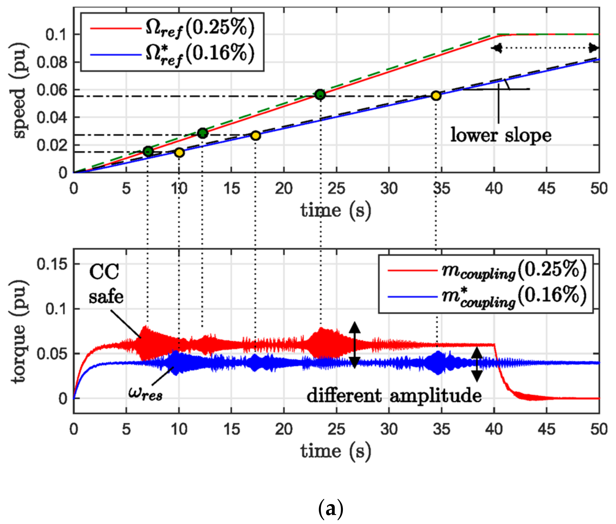
6.2. Feedforward Controller Design

It is possible to improve the control performances adding a feedforward action C(s) into the speed control. In this way, the reference-tracking transfer function F*com(s) becomes (19):
F c o m * ( s ) = R ( s ) + C ( s ) G m o t ( s ) G l o a d ( s ) 1 + R ( s ) G m o t ( s ) .
In order to reduce the overshoot in the response to the load speed Ωload shown in Figure 11, the related feed forward control transfer function C(s) can be computed by imposing (20):
R ( s ) + C ( s ) G m o t ( s ) G l o a d ( s ) 1 + R ( s ) G m o t ( s ) α k p J t o t s + α k p J t o t ,
where α is a design parameter that defines the new dynamics of the command-tracking response in terms of rising time. This leads to the transfer function (21):
C ( s ) = k p s α 1 k p 4 ξ p 2 J t o t s + α k p J t o t .
Once again, the speed step response at constant torque Ωload = 0.1, mload = 0 is evaluated. The benefits of a 2DOF strategy compared with the original regulator R(s) are shown in Figure 13, especially for α = 1 it is possible to mitigate the overshoot, while a higher α decreases the rising time with higher overshoot.
However, the feed forward action C(s) should be designed, minimizing the tracking error of the closed-loop etr(s) (22):
e tr ( s ) = Ω r e f Ω l o a d = 1 F c o m * ( s ) Ω r e f .
According to the CC speed profile, a useful criterion is to evaluate the steady-state error est(s) through the final value theorem in the following cases:
  • When a speed step reference Ωref(s) = h/s is applied, where h represents the step size (e.g., h = 1):
e s t ( s ) = l i m s 0 s e t r 1 s = l i m s 0 s 1 F c o m * ( s ) 1 s = 0
  • When a speed ramp reference Ωref(s) = h/s2 is applied:
e st ( s ) = lim s 0 s 1 F c o m * ( s ) h s 2 = h α k p J t o t .
For the ramp speed reference, to obtain est(s) = 0 the order of C(s) should be in a higher order. Keeping a relative zero-grade, Equation (20) can be rewritten as in (25), where it is used for a second order type:
R ( s ) + C ( s ) G m o t ( s ) G l o a d ( s ) 1 + R ( s ) G m o t ( s ) 2 α h s + α 2 h 2 s 2 + 2 α h s + α 2 h 2 .
This leads to a new C*(s) defined in (26):
C ( s ) = J t o t h s 2 α 1 s + h α 2 1 4 ξ p 2 s + α h 2 ,
where the new closed-loop transfer function differs from the previous one, due to the double pole at s =αhs. In Figure 14, the different choices of α for a speed ramp of a 1% slope are shown.
Different actions, summarized by Copt(s) = F{C(s), C*(s)}, could be applied according to the given reference. Evaluating the actual slope of the speed reference Ωref, a simple algorithm can be executed to select a proper feedforward action, or to reduce the ramp slope. A pseudocode example is given in Algorithm 1.
Algorithm 1. Feedforward Adaptation Pseudocode.
1: α = 1&h = 0.1 ← according to Figure 13 and Figure 14
2: x = dΩref/dt ← it could be discretized
3: if x > 0 then
4: if x ≥ 20% then ← assuming a step
5: Copt(s) = C(s) ← according to (20)
6: else if 0 < x ≤ 1% then ← keeping limit to 1%
7: Copt(s) = C*(s) ← according to (23)
8: else
9: lowerref,t) ← decrease the ramp* slope
10: goto 3
11: else if x < 0 then
12: x = |x| and goto 3
13: else if x = 0 then goto 3
This criterion can be extended to different reference profiles by solving an optimization problem aimed to setpoint tracking, e.g., using an H2 approach: min + e tr ( s ) 2 2 where . 2 stands for the 2-norm.
A ramp command excites the first TNF by running through the critical speeds Ωcrit(i). The applied torque mcoupling leads to shaft failures if the maximum oscillations amplitude Mm(t) exceeds the crack boundary [10]. From Table 1, it follows that this maximum value should respect (27):
M m ( t ) = max m c o u p l i n g ( t ) 10 % m r a t .
According to (27), a slope limit of 1% is followed for the system under analysis.
If the slope is greater than 1%, according to Algorithm 1, the reference will be modified in order to have a lower ramp, even if this modification changes the settling time as a side effect. It is not useful to change the slope only where there are localized critical speeds, due to the introduction of some additional ramps with higher slopes (e.g., 1.23%) that aim to follow the reference. The comparison between these two strategies is shown in Figure 15.

7. Control Stability and Robustness

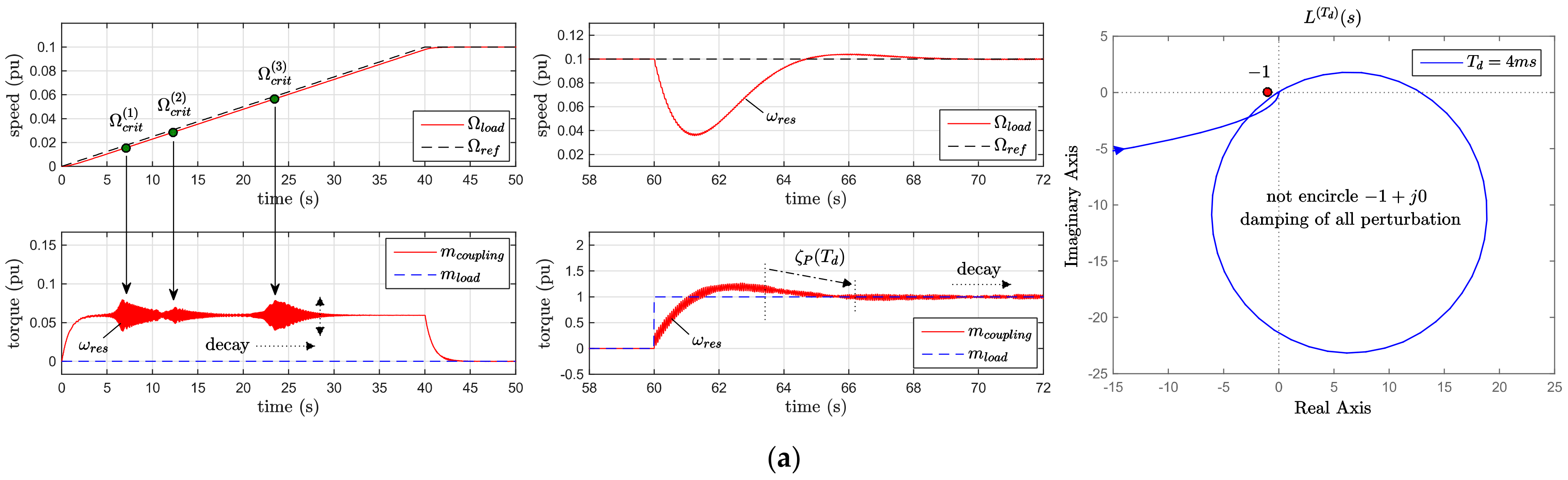
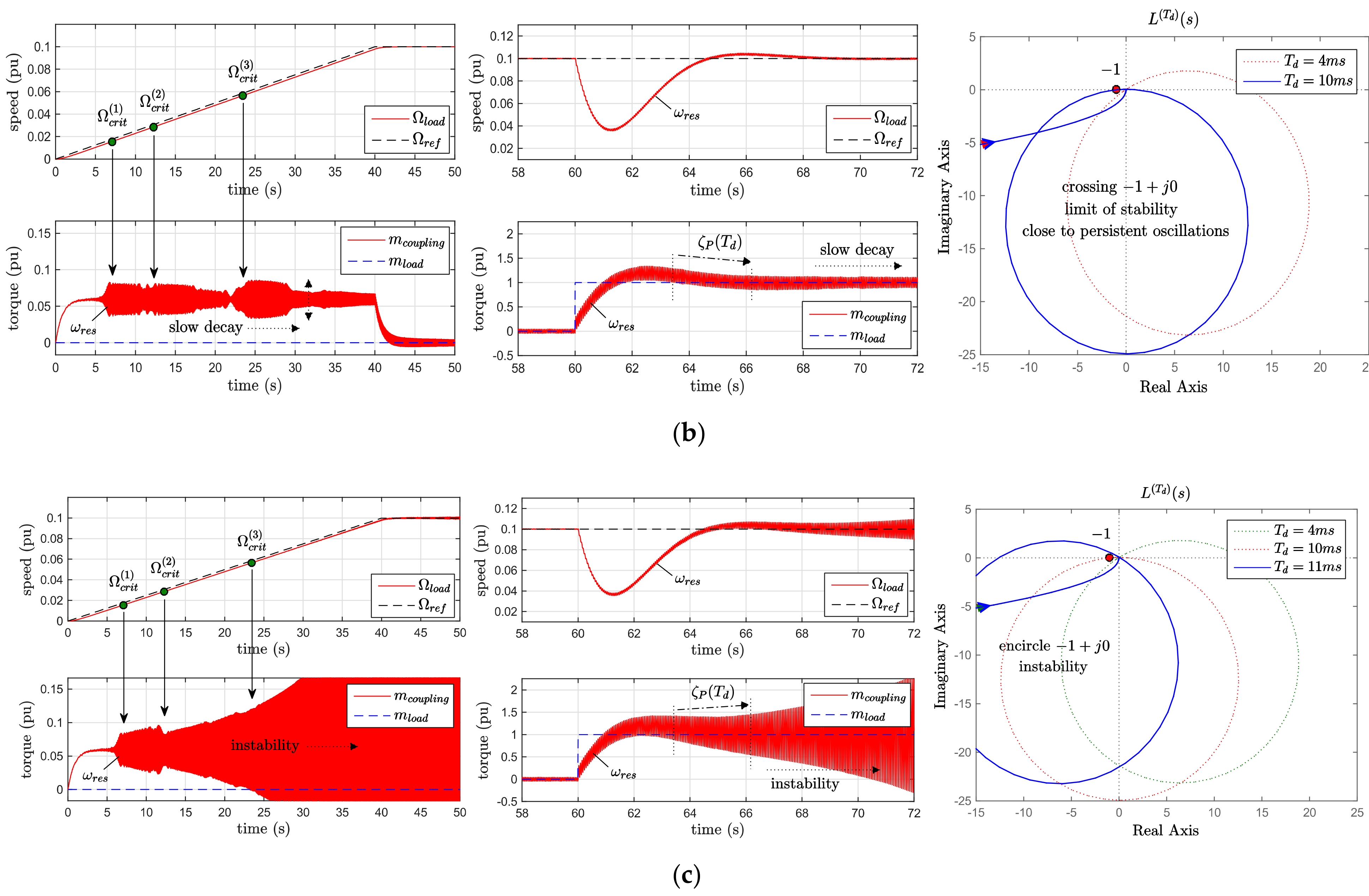
7.1. Nyquist Analysis

Implementing the control algorithm in an industrial DSP leads to time delays due to continuous/discrete-time conversion and integration methods [13,20,21,22,23]. Latencies modify the damping action on the first TNF due to the decreasing effect of the overall closed-loop stability. Time delays can be roughly split into torque-actuation delay Tt, located in the inner torque control transfer function T(s), and speed-computation delay Tm, located in the estimator transfer function E(s). They both can be modeled as first order transfer functions (28) (Figure 8).
T ( s ) : m m o t = m r e f e s T t E ( s ) : Ω ^ m o t = Ω m o t e s T m e T i 1 s T i ( i = t , m ) ,
The behavior of the system can be analyzed through a Nyquist analysis performed on the open-loop transfer function L(s) (12). This is useful to compute a critical time delay Tcr that gives the maximum latency after the stability is lost. Defining a total system delay as Td = Tt + Tm, from (12) this follows (29):
L ( T d ) . ( s ) = L ( s ) e s T d for T d = 0 , , T cr ,
Increasing Td, the vibrating behavior changes in terms of higher amplitude and time–decay, both for critical speeds crossing and step response, as shown in Figure 16. We identified Tcr ≅ 10 ms as the critical value for the system under analysis; if Td < Tcr the system results are stable, but the decaying behavior depends on Td. This sensitivity to Tcr is fundamental to choose a proper sampling time for the discretization onto a DSP.

7.2. Process Damping and Characteristics

A novel descriptive method to analyze the process damping ζP of (7) could be based on the sensitivity to time-delay of reference tracking transfer function F*com(s) [24,25,26,27,28]. The denominator DF(s) of this transfer function has further terms in addition to Gmot(s), with the closed-loop poles characterized as in (30):
D F ( s ) = s 2 + 2 ζ 1 ω 1 s + ω 1 2 s 2 + 2 ζ 2 ω 2 s + ω 2 2 ω 1 , ζ 1 dominant poles ω 2 , ζ 2 { J m o t , J l o a d , K e l , C e l ζ m e c h , k p , k i , ω 1 , ζ 1 } .
If some mechanical parts are changed (e.g., higher CC size ≠ Jload, bigger motor ≠ Jmot, lifetime of the shaft ≠ Kel, Cel), they lead to different {kp,ki} until the worst case is reached: a (ω2, ζ2) close to (ω1, ζ1). Indirectly, the mechanical characteristics can be a positive/negative help to damp the first TNF through ζmech. Similarly, the intrinsic behavior of the motor can add an electromagnetic damping ζelet. Such dynamics can be model as a resonating transfer function given in (31), with an electrical resonance at ωelet.
M ( s ) = μ ω e l e t 2 s 2 + 2 ζ e l e t ω e l e t s + ω e l e t 2
ζelet and ωelet can be computed from an FEM analysis of the electrical side only [2,26,29]. Usually, in CC trains ζelet is negligible compared with ζmech, which is higher due to large Jmot, Jload. In addition, ωelet is located at higher frequency, on the contrary to ωmech. However, even without changes in the electrical or mechanical parts, ζP changes because the control strategy affects the impact of ζmech, ζelet. Considering the latency effect of Td, from (19), it follows (32):
F c o m ( T d ) ( s ) = R ( s ) + C i ( s ) G m o t ( s ) G l o a d ( s ) e s T d 1 + R ( s ) G m o t ( s ) e s T d ,
As shown in Figure 17, increasing the time-delay, the magnitude of the resonance is increased, and this produces a higher amplitude of the first TNF oscillations.
As a first approximation, the resonating behavior at s = j ωres can be described as in (33), where μ = 1 for simplicity.
F c o m ( T d ) ( s ) s = j ω r e s μ ω r e s 2 s 2 + 2 ζ P ω r e s s + ω r e s 2 s = j ω r e s ,
Exploiting the right side of (33) follows a description of ζP(Td) as a function of Td through | F c o m T d s | s = j ω r e s , as in (34).
ζ P ( T d ) = 1 2 Im 1 F c o m ( T d ) ( s ) s = j ω r e s ,
where ζP(Td) is computed using a polynomial curve fitting from samples of (34), changing Td = 0, , Tcr inside the stable region, as shown in Figure 18. This approach allows us to consider the electrical and mechanical design, in addition to the control topology. For example, changing the motor inertia to Jmot * = 10 Jmot, this follows ω*resωres and the stability boundary increases from Tcr to T*cr. As shown in Figure 18, with the same amount of delay, ζ*P (Td) is less sensitive to Td.

8. HIL Experimental Setup

The experimental setup consists of a HIL in a master–slave configuration. A master board is used to implement the control algorithm, and dynamic models for VSI (the DC-link is assumed constant), motor and estimator units. The control algorithm is partially translated from MATLAB/Simulink into C-code, and completed with an assembly-code, then compiled onto a Motorola DSP 24-bit word. A slave board is used to implement the mechanical model, process boundaries and load a torque profile. The boards allow four sampling times Ts from 25 μs to 2 ms, used for backward-discretization. The most sensitive operations are computed at the highest Ts. The communications are based on fibre-optic links. This HIL provides a rapid prototyping platform to test the different speed profiles earlier analyzed in simulation. An overview is shown in Figure 19.
The CC reference profile given in Figure 2 is evaluated with different C(s) and C*(s), as shown in Figure 20. The simulation agrees with the HIL results: there are similar torsional vibrations in terms of amplitude and time–decay both on critical speed crossings and step responses. The torque mcoupling constraint is respected due to a speed ramp of 0.5% and 1%, respectively, validating the early analyzed approach. The process damping is ζP(7 ms) ≅ 0.3. For effective simulations, an additional white noise generator should be added because the HIL presents a greater noise than actual simulation, i.e., due to hardware implementation delays. Comparison between HIL and simulation results are reported in Table 4.
In addition to time-domain simulations, the power spectra of the coupling torque is evaluated through a waterfall diagram. The diagrams in Figure 20 exhibit the spectrum variation over time, by plotting a series of frequency-domain spectrums calculated during a consecutive time window of 15 s. This method is accurate if it is considered as a steady-state signal. By applying a Hanning window in a range 55–70 s, it follows a noisier waterfall diagram for the HIL than the other, but there are clear first TNF peak lines for both.

9. Conclusions

This paper presents a complete design procedure and performance analysis of a motor drive control, in order to minimize oscillations and improve system reliability. A model-based pole placement design method and an adjustable feedforward action of a 2DOF speed control have been presented. Sensitivity to time delays, noise and parameter changes were analyzed by means of Nyquist diagrams, the process damping descriptive method, time-domain simulations and waterfall diagrams. Simulations and HIL experiments showed that the designed controller achieved good reference tracking for both step and ramp commands, as well as a robust load torque rejection to valve opening for an industrial compressor system.

Author Contributions

M.R., M.S.C., M.M. have contributed in the same way to all the paper sections. All authors have read and agreed to the published version of the manuscript.

Funding

This research received no external funding.

Institutional Review Board Statement

Not applicable.

Informed Consent Statement

Not applicable.

Data Availability Statement

Not applicable.

Acknowledgments

The authors would like to thank the ABB MV-Drives DMDR-MDC in Turgi Switzerland, in particular Christian Stulz, Halina Burzanowska, Pieder Jorg and Corrado Fiordimela. We would also like to thank the Delta JS Switzerland, in particular Joachim Schmied for rotordynamics simulation.

Conflicts of Interest

The authors declare no conflict of interest.

References

  1. Muszynski, R.; Deskur, J. Damping of torsional vibrations in highdynamic industrial drives. IEEE Trans. Ind. Electron. 2010, 57, 544–552. [Google Scholar] [CrossRef]
  2. Holopain, T.; Repo, A.; Niiranen, J. Electromechanical interaction in torsional vibrations of drive train systems including an electrical machine. In Proceedings of the 8th IFToMM International Conference on Rotordynamics, Seoul, Korea, 12–15 September 2010; p. 933. [Google Scholar]
  3. Del Puglia, S.; Franciscis, S.; Van de Moortel, S.; Jörg, P.; Hattenbach, T.; Sgrò, D.; Antonelli, L.; Falomi, S. A Torsional Interaction Optimization in a LNG Train with Load Commutated Inverter. In Proceedings of the 8th IFToMM International Conference on Rotor Dynamics, Seoul, Korea, 12–15 September 2010. [Google Scholar]
  4. Song-Manguelle, J.; Schröder, S.; Geyer, T.; Ekemb, G.; Nyobe-Yome, J.M. Prediction of mechanical shaft failures due to pulsating torques of variable-frequency drives. IEEE Trans. Ind. Appl. 2010, 46, 1979–1988. [Google Scholar] [CrossRef]
  5. Mauri, M.; Rossi, M.; Bruha, M. Generation of Torsional Excitation in a Variable-Speed-Drive System. In Proceedings of the IEEE 23nd International Symposium on Power Electronics, Electrical Drives, Automation and Motion, SPEEDAM, Capri Island, Italy, 22–24 June 2016. [Google Scholar]
  6. Szabat, K.; Orlowska-Kowalska, T. Vibration suppression in a twomass drive system using PI speed controller and additional feedbacks—Comparative study. IEEE Trans. Ind. Electron. 2007, 54, 1193–1206. [Google Scholar] [CrossRef]
  7. Harnefors, L.; Saarakkala, S.E.; Hinkkanen, M. Speed control of electrical drives using classical control methods. IEEE Trans. Ind. Appl. 2013, 49, 889–898. [Google Scholar] [CrossRef]
  8. Saarakkala, S.E.; Hinkkanen, M.; Zenger, K. Speed control of two-mass mechanical loads in electric drives. In Proceedings of the IEEE Energy Conversion Congress and Exposition, ECCE, Raleigh, NC, USA, 15–20 September 2012; pp. 1246–1253. [Google Scholar]
  9. Saarakkala, S.E.; Hinkkanen, M. State-space speed control of two mass mechanical systems: Analytical tuning and experimental evaluation. IEEE Trans. Ind. Appl. 2014, 50, 3428–3437. [Google Scholar] [CrossRef] [Green Version]
  10. Rossi, M.; Marco, M.; Castelli-Dezza, F.; Carmeli, M.S. Discrete multi-layer estimator implementation for sensorless control of elastic drive systems—An industrial case study. In Proceedings of the 14th IMEKO TC10 Workshop on Technical Diagnostics, Milan, Italy, 27–28 June 2016. [Google Scholar]
  11. Schramm, S.; Sihler, C.; Song-Manguelle, J.; Rotondo, P. Damping torsional interharmonic effects of large drives. IEEE Trans. Power Electron. 2010, 25, 1090–1098. [Google Scholar] [CrossRef]
  12. Brock, S.; Deskur, J. The problem of measurement and control of speed in a drive with an inaccurate measuring position transducer. In Proceedings of the International Workshop on Advanced Motion Control, Trento, Italy, 26–28 March 2008; Volume 1, pp. 132–136. [Google Scholar]
  13. Ikeda, H.; Hanamoto, T.; Tsuji, T. Digital Speed Control of Multi-Inertia Resonant System Using Real Time Simulator. In Proceedings of the International Conference on Electrical Machines and Systems, Seoul, Korea, 8–11 October 2007; Volume 10, pp. 1881–1886. [Google Scholar]
  14. Holopain, T.; Niiranen, J.; Jörg, P.; Andreo, D. Electric Motors and Drives in Torsional Vibration Analysis and Design. In Proceedings of the 42nd Turbimachinery Symposium, Houston, TX, USA, 1–3 October 2013. [Google Scholar]
  15. Zhang., G.; Furusho, J. Speed control of two-inertia system by PI/PID control. IEEE Trans. Ind. Electron. 2000, 47, 603–609. [Google Scholar] [CrossRef]
  16. A.P.I. Standard. Tutorial on the API Standard Paragraphs Covering Rotor Dynamics and Balance: An Introduction to Lateral Critical and Train Torsional Analysis and Rotor Balancing; American Petroleum Institute (API): Washington, DC, USA, 1996. [Google Scholar]
  17. DeWinter, F.; Grainger, L. A practical approach to solving large drive harmonic problems at the design stage. IEEE Trans. Ind. Appl. 1990, 26, 1095–1101. [Google Scholar] [CrossRef]
  18. Ferretti, G.; Magnani, G.; Rocco, P. Some fundamental limitations in the control of two-mass systems. In Proceedings of the IEEE 2009 International Conference on Mechatronics, ICM, Malaga, Spain, 14–17 April 2009. [Google Scholar]
  19. Harnefors, L. Proof and application of the positive-net-damping stability criterion. IEEE Trans. Power Syst. 2011, 26, 481–482. [Google Scholar] [CrossRef]
  20. Kocur., J.; Muench, M. Impact of Electrical Noise on the Torsional Response of VFD Compressor Trains. In Proceedings of the Proceedings of the Forty First Turbomachinery Symposium, Houston, TX, USA, 24–27 September 2012. [Google Scholar]
  21. Lecchini, A.; Campi, M.C.; Savaresi, S.M. Virtual reference feedback tuning for two degree of freedom controllers. Int. J. Adapt. Control Signal Process. 2002, 16, 355–371. [Google Scholar] [CrossRef] [Green Version]
  22. Lipo, T.A.; Krause, P.C. Stability analysis of a rectifier-inverter induction motor drive. IEEE Trans. Power Appar. Syst. 1969; PAS-88, 55–66. [Google Scholar]
  23. Rossi, M.; Mauri, M.; Carmeli, M.S.; Castelli-Dezza, F. Latency Effect in a Variable Speed Control on Torsional Response of Elastic Drive Systems. In Proceedings of the IEEE 22nd International Conference on Electrical Machines, ICEM, Lausanne, Switzerland, 4–7 September 2016; pp. 2282–2288. [Google Scholar]
  24. Rotondo, P.; Andreo, D.; Falomi, S.; Jörg, P.; Lenzi, A.; Hattenbach, T.; Fioravanti, D.; De Franciscis, S. Combined Torsional and Electromechanical Analysis of an LNG Compression Train with Variable Speed Drive System. In Proceedings of the 38th Turbimachinery Symposium, Houston, TX, USA, 14–17 September 2009; pp. 93–102. [Google Scholar]
  25. Simond, J.J.; Sapin, A.; Tu Xuan, M.; Wetter, R.; Burmeister, P. 12-Pulse LCI synchronous drive for a 20 MW compressor modeling, simulation and measurements. IAS Annu. Meet. 2005, 4, 2302–2307. [Google Scholar]
  26. Szabat, K.; Orlowska-Kowalska, T.; Dybkowski, M. Indirect Adaptive Control of Induction Motor Drive System with an Elastic Coupling. IEEE Trans. Ind. Electron. 2009, 56, 4038–4042. [Google Scholar] [CrossRef]
  27. Tamaoki, T.; Takanezawa, M.; Lu, Z.; Xiao, S.; Kimoto, M.; Morita, N. A study for on-line transfer function analysis, in realizing higher speed response adjustment, in association with variable speed rolling mill motor drive system. In Proceedings of the International Power Electronics Conference—ECCE Asia, IPEC, Sapporo, Japan, 21–24 June 2010; pp. 2516–2519. [Google Scholar]
  28. Thomsen, S.; Hoffmann, N.; Fuchs, F.W. PI Control, PI-Based State Space Control, and Model-Based Predictive Control for Drive Systems with Elastically Coupled Loads—A Comparative Study. IEEE Trans. Ind. Electron. 2011, 58, 3647–3657. [Google Scholar] [CrossRef]
  29. Wachel, J.C.; Szenasi, F.R. Analysis of Torsional Vibrations in Rotating Machinery. In Proceedings of the 22sd Turbomachinery Symposium, Dallas, TX, USA, 14–16 September 1993. [Google Scholar]
Figure 1. Centrifugal compressor schema.
Machines 09 00374 g001
Figure 2. Reference signals.
Machines 09 00374 g002
Figure 3. Vibrating behaviour of the drive train. (a) Bode diagrams; (b) torsional vibration mode.
Machines 09 00374 g003
Figure 4. Exploit of the electrical topology of a VSD.
Machines 09 00374 g004
Figure 5. Motor torque harmonic content. (a) Air-gap torque time behavior; (b) air-gap torque harmonics contents.
Machines 09 00374 g005
Figure 6. Campbell diagram of the analyzed system.
Machines 09 00374 g006
Figure 7. Damping influences at critical speeds: critical frequencies representation in the Campbell and Bode diagrams.
Machines 09 00374 g007
Figure 8. Control scheme.
Machines 09 00374 g008
Figure 9. Pole placement assignment cases. (a) Poles position; (b) pole placement design regions.
Machines 09 00374 g009
Figure 10. Controller parameters 3D surfaces. (a) kp design surfaces; (b) ki design surfaces.
Machines 09 00374 g010aMachines 09 00374 g010b
Figure 11. Bode diagram with kp = 10 and ki = 6.5. (a) Open-loop transfer function L(s) Bode diagram; (b) command-tracking transfer function Fcom(s) Bode diagram. Red lines represent rigid behavior.
Machines 09 00374 g011
Figure 12. Step responses with R(s). (a) Speed reference step changing response; (b) load torque step changing response.
Machines 09 00374 g012
Figure 13. First order transient comparison according α in terms of speed response and torque response.
Machines 09 00374 g013
Figure 14. Second order transient comparison according to α, in terms of speed response and torque response.
Machines 09 00374 g014
Figure 15. Energy consideration for ramp speed reference. (a) Speed and torque system behavior; (b) speed reference possible modifications.
Machines 09 00374 g015aMachines 09 00374 g015b
Figure 16. System response (torque and speed) and stability analysis with different Td: (a) Td = 4 ms; (b) Td = 10 ms; (c) Td = 11 ms.
Machines 09 00374 g016aMachines 09 00374 g016b
Figure 17. Latency impact on F(Td)com(s) varying Td.
Machines 09 00374 g017
Figure 18. Process damping description as a function of Td.
Machines 09 00374 g018
Figure 19. HIL in back-to-back configuration (Motorola DSP 24-bit word); (1) master board; (2) slave board (load model); (3) signaling interfaces; (4) interface boards; (5) emergency panel.
Machines 09 00374 g019
Figure 20. Comparison between simulation (a) and HIL (b) results.
Machines 09 00374 g020
Table 1. System parameters.
Electric Data
Voltage vrat (kV)6
Current irat (A)931
Frequency fline (Hz)50
Speed Ωrat (rpm)1492.45
Pole pairs npp2
Mechanical Data
IM inertia Jmot (Nms2/rad)510
Load inertia Jload (Nms2/rad)226.3
Stiffness Kel (Nm/rad)1.347 × 107
Damping Cel (Nm s/rad)100
Static friction fs (Nm)0.95
Dynamic friction fv (Nms2/rad2)10−4
Crack limit ad mrat (%)10
Table 2. System critical speed.
Supply Frequency fline (Hz)50 50 50
Resonance first TNF (Hz)17 17 17
Resonance ωres (rad/s)106.76 106.76 106.76
Integer (m, ±k) (0, +6) (0, +12) (0, +18)
Harmonics nk 6th 12th 18th
Critical Speeds Ω(i)crit (pu)(3) 0.056 (2) 0.028 (1) 0.019
Table 3. Feedback coefficients design.
p1,2Pulsation ω1 (Rad/s)10.5
Damping ζ1 0.55
Gain kp (pu)10
Gain ki (pu)6.5
p3,4Pulsation ω2 (rad/s)112.05
Damping ζ2 0.34
Table 4. Maximum oscillations Mm (t).
SimulationCritical Speeds Ω(1)crit Mm ≅ 4%
Ramp command (0.1 → 0.2) Mm ≅ 2%
Step commandMm ≅ 3.5%
HILCritical speeds Ω(1)crit Mm ≅ 4.5%
Ramp command (0.1 → 0.2) Mm ≅ 2.2%
Step commandMm ≅ 3.5%
Noise level % ≅1.6%
Publisher’s Note: MDPI stays neutral with regard to jurisdictional claims in published maps and institutional affiliations.

