Abstract
Industrial robots have advantages in the processing of large-scale components in the aerospace industry. Compared to CNC machine tools, robot arms are cheaper and easier to deploy. However, due to the poor consistency of incoming materials, large-scale and lightweight components make it difficult to automate robotic machining. In addition, the stiffness of the tandem structure is quite low. Therefore, the stability of the milling process is always a concern. In this paper, the robotic milling research is carried out for the welding pre-processing technology of large-scale components. In order to realize the automatic production of low-conformity parts, the on-site measurement–planning–processing method is adopted with the laser profiler. On the one hand, the laser profiler hand–eye calibration method is optimized to improve the measurement accuracy. On the other hand, the stiffness of the robot’s processing posture is optimized, combined with the angle of the fixture turntable. Finally, the experiment shows the feasibility of the on-site measurement–planning–processing method and verifies the correctness of the stiffness model.
1. Introduction
Large-scale components are commonly found in the aerospace and shipbuilding fields. The manufacturing requirements of these components require large-scale machine tools. However, large-scale or special-purpose machine tools are expensive. The deployment of large components on the machine tool is time-consuming and laborious [1,2]. Therefore, it is difficult to meet the demand. In addition, some workpieces have to use machine tools because manual work cannot guarantee product quality, though they do not have high accuracy requirements. Therefore, industrial robots are widely used in this case. Industrial robots have incomparable flexibility and price advantages to CNC machine tools [3,4,5]. They are easy to deploy and have a large working space. They have gradually become key pieces of equipment in the field of aerospace manufacturing. However, their shortcomings are also obvious. For example, the stiffness of the tandem structure is poor, the programming difficulty is often higher than that of the CNC system, and it is not easy to automate the incoming materials with low consistency. Especially in the milling process, the serial structure of industrial robots makes machine chatter unavoidable. Thus, the chatter problem has always been a research hotspot [6,7,8,9].
This paper focuses on the robotic processing of large structural parts in the aerospace field. Since large-size components are often welded by multiple parts, bevel processing is indispensable in the welding process. However, the bevel processing is often carried out manually. Because of its large amount of removal, workers need to finish this part by working in a dusty and noisy environment for hours. In addition, due to the low stiffness of this lightweight component, the consistency of its previous processing is very poor. Furthermore, the workpiece has no positioning reference, which brings great difficulties to automation. In this paper, the authors will accomplish robotic bevel processing for low-consistency workpieces automatically. At the same time, considering that the processing method is milling, the stiffness performance of the robot needs to be optimized to improve processing stability.
Due to the structural characteristics and manufacturing process characteristics of large lightweight components, the incoming consistency of the bevel processing process is low. This, together with no benchmark fixtures, results in barriers to deploying automated production. Therefore, the robot cannot process with an inflexible program such as traditional CNC milling.
In this paper, a flexible robotic milling process framework is proposed, as shown in Figure 1. The robot carries a laser line sensor to scan and obtain the point cloud of the workpiece profile. As a laser profiler can provide high-accuracy data, the point cloud data can be processed and applied to trajectory planning directly.

Figure 1.
A flexible robotic milling process framework.
According to bevel processing technical requirements, the 3D cameras are not suitable for milling applications because of their low accuracy. However, the hand–eye calibration method of the profiler based on a laser line is not widely applied. To improve detection accuracy, a hand–eye calibration method for a laser line sensor based on Genetic Algorithms (GA) is proposed.
Compared to CNC, the disadvantages of robotic milling are obvious. The low stiffness aggravates chatter during the milling process. Thus, in this section, the effect of stiffness on processing is considered. Robotic milling stability is improved by optimizing the manipulator’s processing posture. On the other hand, the velocity of the manipulator’s trajectory is also optimized to improve the processing efficiency.
The remainder of the paper is organized as follows: The related works of several key techniques are introduced in Section 2. Section 3 will present a novel hand–eye calibration method. Section 4 will provide the feature analysis method and path planning based on point cloud data of the actual part. The milling postures will be optimized in Section 5 based on stiffness modeling. The results and discussion of the system experiment will be shown in Section 6. Section 7 will conclude the paper.
2. Related Works
This section includes the robot hand–eye calibration method for a laser profiler and research on the stiffness of robots.
Aerospace structural parts often require online measurements to obtain the structural characteristics of the current workpiece. According to different applications, the accuracy requirements are different, and the sensors are also different. In the existing research, there are many methods to measure the whole workpiece or the region of interest using robots combined with measurement sensors. Kuss et al. used a 3D camera to achieve a three-dimensional measurement of structural steel workpieces [10] and completed the deburring process according to the measurement results. Han et al. used a system of robots and 3D cameras to measure the three-dimensional shape of the workpiece on the forging production line [11]. Yu designed the line laser rotating mirror scanning equipment and successfully applied it to the scanning of the car body in white by the robot system [12]. Wang et al. used a mobile robot combined with a 3D camera to increase the scanning range of the robot and realized the scanning of the wind turbine blade model [13]. Ge et al. used robots and line laser sensors to realize the welding seam of the steel pipe workpiece via online measurement and removal [14]. Guo et al. used robots and line laser sensors to measure and remove spiral welds on steel pipes [15]. Among them, it can be found that due to its limited accuracy, 3D cameras are often used in applications where precision requirements such as deburring and polishing are not high. Sensors based on the principle of laser imaging, usually used for quality inspection or welding seam processing, requires high precision or simple scanning methods. In this paper, for bevel processing, the accuracy requirements are relatively high, and 3D cameras are not suitable. Therefore, the laser profile sensor is the first choice.
Generally speaking, in order to adapt to the task of 3D measurement of large-scale components, the system adopts the form of “eye on hand”. Hand–eye calibration methods currently mainly include traditional methods, optimization methods, and some probability-based methods, but most of them are for camera sensors. The research ideas of hand–eye calibration for a laser profiler are similar and simple. A typical calibration method is to use a robot to measure a standard ball in multiple poses [16,17,18,19] and construct a similar equation to solve it. In addition, some scholars use some special-shaped calibration objects, such as disc-shaped [20], X-shaped [21] and multi-step calibration objects [22]. Carlson et al. used a three-orthogonal plane method for calibration [23], and Sharifzadeh et al. improved this by using a single plane to achieve convenient and stable calibration [24]. However, for the measurement task, what needs to be obtained is the 3D reconstruction result of the measured object. From the perspective of 3D reconstruction, there are many systematic errors, including distortion and scattering, which cannot be solved by traditional methods. Therefore, on this basis, optimization methods may be more suitable to improve data accuracy.
Industrial robots are composed of tandem rotary joints. Although this structure is beneficial to increase the working space of the robot, it will result in significantly low stiffness characteristics. The cutting force acting on the end of the robot arm during the machining process will cause undesired displacements. Due to the low stiffness, the error produced during the machining process accounts for the main proportion of the machining error [25]. Therefore, a lot of research has focused on the stiffness modeling and stiffness error compensation of the robot. Stiffness modeling methods can be divided into two categories: virtual joint method (VJM), which describes elastic components as lumped parameter models [26,27], and finite element analysis (FEA), which calculates elastic deformation based on computer finite element-aided design tools [28,29,30]. The virtual joint method can easily obtain the stiffness model of the robot, but the accuracy is not as good as the finite element method. The main advantage of the finite element analysis method is its higher accuracy, but it requires higher computing power support and higher modeling skills. Gong [31] believes that the influence of robot load and the weight of the connecting rod on the deformation of the joint is significantly greater than the flexible deformation of the connecting rod, so most of the literature only considers the influence of the flexible joint deformation [31,32,33]. Khalil [34] uses the cantilever beam model to consider the flexible deformation of the connecting rod, which is too complex to be suitable for engineering applications. Therefore, the virtual joint method is widely used in robot processing applications because of its high computational efficiency and acceptable accuracy. Salisbury [35] first proposed a robot stiffness model. The transmission components of each joint of the robot (such as reducer, actuator, etc.) are the main sources of flexible deformation of the robot. A virtual torsion spring is used to represent the stiffness of each joint, thereby establishing a classic stiffness model. However, this model is only valid when the robot has no load. Therefore, Chen et al. proposed a Conservative Congruential Transformation (CCT) [36,37]. CCT describes the relationship between the Cartesian stiffness matrix and the joint stiffness matrix and considers the displacement change of the robot caused by the load on the end of the robot. This paper is based on this method to identify the stiffness of the robot. The robot processing path is optimized using this stiffness index.
3. Hand–Eye Calibration
3.1. Modeling
The robot hand–eye calibration is used to obtain the coordinate system of the sensor relative to the robot end. The calibration model of the robot line laser scanning system is shown in Figure 2. In order to calibrate the hand–eye relationship, the following coordinate system needs to be established: stands for robot base coordinate system; stands for robot tool coordinate system, where is the axe of robot flange center; stands for the profiler coordinate system, where is perpendicular to the laser plane.
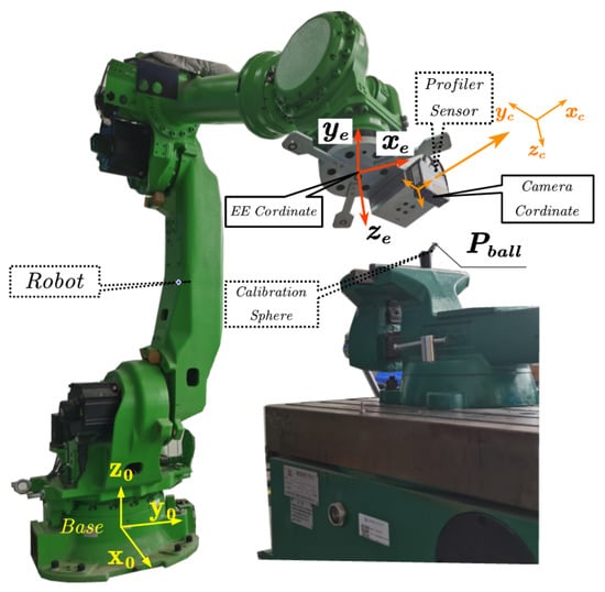
Figure 2.
The calibration model of the robot line laser scanning system.
It is easy to obtain the transformation relationship through the kinematics between and . Therefore, the goal is to solve the transformation relationship between and . Let be the center of calibration ball in , and be that in . Therefore, the relationship is:
Equation (1) can be transformed into the following form:
where r and t denote the rotation and translation of T.
The relative relationship between the center of the laser calibration sphere and the profiler coordinate system is shown in Figure 3. Therefore, according to the measurement principle of the line laser sensor, we use the least square method to solve the radius and the secant plane center (only x and z of ) of the light plane and the laser calibration sphere. Thus, h (y of ) in Figure 4 can be calculated with and .

Figure 3.
The relative relationship between the center of the laser calibration sphere and the profiler coordinate system.
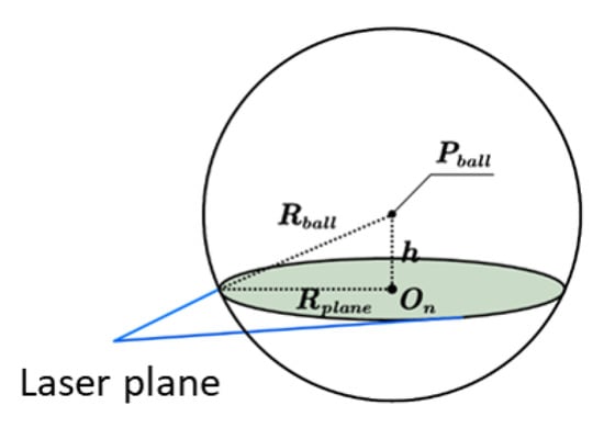
Figure 4.
The measurement principle of the line laser sensor.
As the calibration sphere is fixed, is constant in . To solve , equations can be set from different positions and postures of the manipulator, that is:
3.2. Solution
As the analytical method is applied, the results show a great degree of dispersion in y values of . Therefore, a solution based on a Genetic Algorithm (GA) is proposed for the calibration method to improve the accuracy. GA is an optimization process that is suitable for a wide range of values, many parameters and nonlinearity. Since directly solving the six parameters of the hand–eye relationship is easy to converge to the local optimum, this part adopts the method of applying GA to solve the rotation component and translation component, respectively.
As the initial value of the rotation and translation components are calculated from the designed model, the objective function and individual fitness functions are designed as follows. The rotation matrix of the x component is:
Then the rotation of is:
Thus, the objective function can be expressed as:
where denotes the Euclidean norm, and denote Euler angle inputs. Floating point encoding is adopted instead of binary encoding to shorten the encoding length and improve the efficiency. The individual fitness function can be expressed as:
Let , while is calculated above. The same is true for the translation component; the objective function can be expressed as:
3.3. Calibration Results
To obtain a reasonable calibration results, 3 time measurements are carried out for each of the 3 postures. The analytical method and GA method are both tried out, so there are 18 groups of data, as shown in Table 1. In Figure 5, calculated sphere centers are shown in an intuitive form. The standard deviation of the sphere centers by analytical method is , while that by the GA method is . It shows that the method based on GA has a good robustness to system errors. The final hand–eye calibration result is = 126.92 mm, = 9.44 mm, = 41.48 mm, r = 60.489, p = −3.813, y = −2.024.

Table 1.
Sphere center results.

Figure 5.
Calculated sphere centers results; (a) analytical method; (b) GA method.
The reason for the inaccuracy of the analytical method is that the diameter of the calibration sphere used in this calibration is a bit small (10 mm), while the repeated positioning accuracy of the robot is 0.2 mm. The sensor’s sensitivity to the light environment and the accumulation of errors, etc., lead to a large deviation between the results of this calibration using the analytical method and the design value. According to the above factors, the authors design the corresponding objective function for the GA on the basis of the analytical method and obtain a more accurate result.
4. Planning Based on Processing Features
4.1. Scanning
The workpiece profile in point cloud data is the precondition of all the analysis jobs. The manipulator carried a profiler to scan the workpiece, which is shown in Figure 6. The main problem is how to align the data obtained from different devices. Specifically, two kinds of data are needed to reconstruct the point cloud data, tool position information from the manipulator and point information from the sensor. For every profile points group , there is a tool position . Therefore, multiple measurements can be expressed as:
where denotes the hand–eye calibration matrix in the previous section, and n denotes the times of measurements. Then, the final point cloud data are fused as .
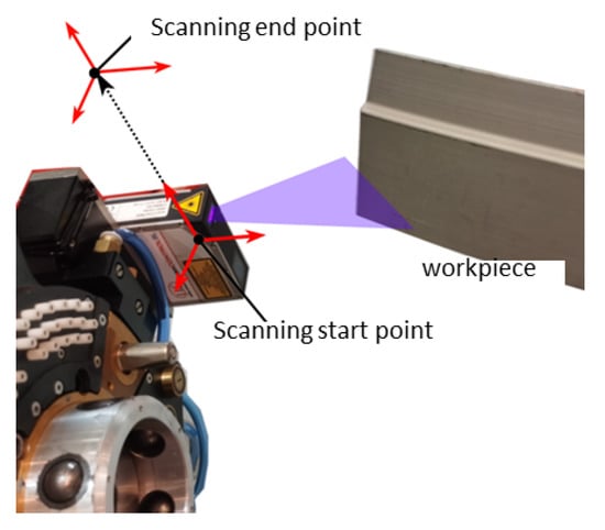
Figure 6.
The installation of a manipulator and a profiler.
However, to reconstruct a high accuracy workpiece model, n needs to be large. Multiple measurements will consume a lot of time. According to the profiler’s communication performance, the data frequency can be 50 Hz. Continuous measurement by a moving manipulator can solve this problem. The manipulator is configured to move in a straight line (easy to interpolate) at a uniform speed. The authors use time stamps to align the sensor data with and . Thus, other can be calculated by interpolation. Then the final point cloud data are computed with Equation (9). Therefore, this method can improve the efficiency significantly.
4.2. Extraction
Figure 7 shows the situation of robotic milling on a workpiece. As the process features are suitable for peripheral milling, the end side face of the workpiece needs to be extracted for tool path planning. In the previous part, the scanned model is made up of 2D profiles. Every profile is one frame, and the edge points are made of vertexes in every frame. As vertex is extremum, it is easy to extract in a 2D plane. Figure 8a,b shows the performance of edge extraction.
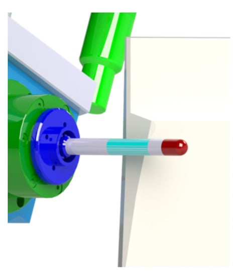
Figure 7.
The situation of robotic milling on the workpiece.
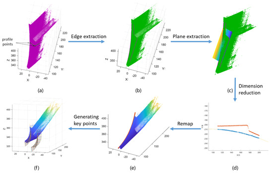
Figure 8.
Tool path planning procedure: (a) rough point cloud data, (b) edge extraction result, (c) plane extraction result, (d) edge extraction in 2D, (e) edge in 2D remapping to 3D, (f) key points on edge.
The least square method, a simple identification method, is used for plane fitting. From the plane expression , the expression in matrix form is:
The objective function is:
4.3. Planning
When considering the cutting amount, the z-axis of the peripheral milling cutter should be planned on the direction of a narrow feather. Then the cutter motion direction y-axis is perpendicular to the z-axis and normal to the extraction plane x-axis. After the coordinate is defined, a series of key points of the tool path can be generated every 1 mm, as shown in Figure 8e.
Finally, to face the requirements of processing, the angle of the edge side face and bevel plane is 40°, and the tool path also needs to be rotated around the z-axis by 40°. Thus one tool path is generated, as shown in Figure 8f, and all other tool paths are spatially translated along the edge side face.
5. Processing Posture Optimization
Mode coupling chatter was identified as the dominant source of vibrations in robotic machining, largely due to the inherent low structure stiffness of an industrial robot. In this section, the authors establish the stiffness model and identify the stiffness matrix. Then, a new evaluation indicator is proposed and applied to optimize the manipulator’s stiffness performance.
Before modeling, three hypotheses should be stated here: (1) The end effector is infinitely stiff. (2) Links of the manipulator are infinitely stiff. (3) All the processing is in a steady state, as the feeding motion is quite slow. Therefore, all the deformations are caused by joint flexibility.
5.1. Cartesian Stiffness Model
In the process of robot grasping objects and operations, is regarded as a measure between the displacement of the robot tool coordinate system and the interaction force when an external force acts on the robot end effector. In the classic stiffness description, it is related to the joint stiffness of robot as follows:
According to the Taylor expansion formula, the relationship between the small force vector and small displacement vector on the end of the manipulator is expressed as (higher-order terms are ignored):
According to the robot Jacobian matrix, can be expressed as:
However, the classic stiffness description is valid only for a quasi-static robot configuration with no loading. During processing, the milling force can cause joint torque. As joint torque can be given by , Equation (13) is substituted into a virtual work principle, which is written as:
The last term can be simplified by using the method proposed by Chen et al., that is:
Thus, the additional stiffness term due to external loading has been incorporated using the Conservative Congruence Transformation (CCT) approach.
5.2. Joint Stiffness Identification
Judging from Equation (17), the joint stiffness is very sensitive to the condition number of the Jacobian matrix. In order to ensure that the stiffness identification program can converge to a stable value, it is necessary to determine the dexterity in each posture to select a posture suitable for stiffness identification.
The physical meaning of the dexterity of a robot is a comprehensive measure of the movement ability in all directions, which is used to measure the flexibility of the robot in various spatial poses. It is defined as:
where are the eigenvalues of , and are the singular values of the Jacobian matrix.
As the dexterity is deeply affected by Axis II and Axis III of the 6 DOF robot, a contour map of under the two axes is given in Figure 9 to analyze the suitable postures. In addition, Axis IV, V, VI are configured at 45° to avoid singular points.
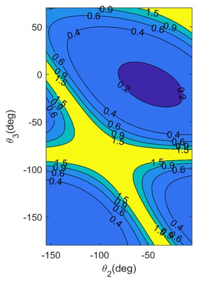
Figure 9.
Contour map of under the two axes.
To simplify the identification, the authors hope to ignore term. Equation (17) shows that the higher the milling force is, the bigger value the gets. A 2000 N force vector and a 200 Nm torque are applied to the end of the manipulator. Here, two indices and are adopted to describe the influence of on based on translational and rotational displacements. They are defined as follows:
and
where and denotes the point-displacements of robot end-effector under milling force with and without considering , respectively. In addition, and denote the small rotations of the robot end-effector under torque with and without considering .
Figure 10 shows the contour map of and on Axis II and Axis III. The darker color means the lower influence. However, all the values of and are tiny. When and 0.0001 rad, the term is considered negligible. Therefore, substitute Equation (12) into Equation (13), the force can be written as:
or
If joint flexibility is expressed as:
Then, by expanding Equation (22), it turns out that:
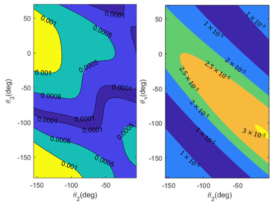
Figure 10.
Contour map of (a) and (b) under the two axes.
Consequently, Equation (24) is the form for force loading tests. According to the analysis above, a posture of higher dexterity and lower influence of is chosen. Then, the joint stiffness can be computed by the amount of applied force values and displacements of the robot’s end-effector. In order to obtain a higher accuracy stiffness matrix of joints, the least squares method will be adopted with multiple measurements. The identification experiment is carried out in Section 6.2.
5.3. Optimization
Suppose the stiffness matrix of joints has been obtained, Cartesian stiffness can be calculated at every posture by Equation (14), thus providing a different measure for the influence of milling force at different postures. Figure 11 shows the robotic milling system, including an industrial robot, an electric spindle (end-effector), and a fixture turntable. In this system, there are two redundant degrees of freedom, rotation of the fixture turntable and rotation of the cutter. Therefore, for the milling job, there are always a series of processing postures gaining better stiffness performance. In addition, two conditions must be met: (1) the postures of the manipulator are solvable, (2) the postures are non-collision.
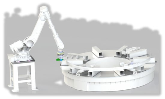
Figure 11.
The robotic milling system.
An optimization problem is defined as follows:
where denotes the rotation offset of the milling cutter and denotes the rotation of the fixture turntable, i denotes the points in the whole tool paths, and denotes 6 angles of the posture in joint space. The objective function is the average of the displacements , which are calculated according to the stiffness equation.
6. Experiments, Results and Discussions
In this section, simulations and experiments are carried out to verify the methods proposed above. This part contains the complete process of the robotic milling system, including measurement and planning, stiffness identification and optimization, and machining test.
6.1. Tool Path Planning
The coordinate system is defined as shown in Figure 12. is the origin of the robot tool coordinate system. is the origin of the processing coordinate system. The industrial robot is ABB IRB6700-150 with a 150 kg payload. Based on the single up-milling tool path generated in Section 4, all the tool paths are planned layer by layer, as shown in Figure 13.
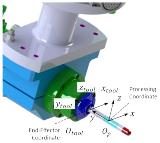
Figure 12.
The tool coordinate system.
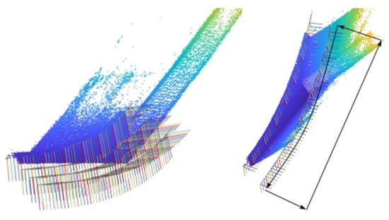
Figure 13.
All the tool paths.
However, not all tool paths cut the workpiece. Considering the processing efficiency, the authors accelerate the motion of the non-cutting path. A velocity planning method is proposed here:
where denotes the minimum distance between the y-axis of the processing coordinate system and the point cloud of the workpiece; and denote the velocity of the cutter at non-cutting points; R denotes the radius of the cutter.
Figure 14 shows the performance of the non-cutting path velocity planning. The darker color denotes a lower velocity and lighter denotes higher.
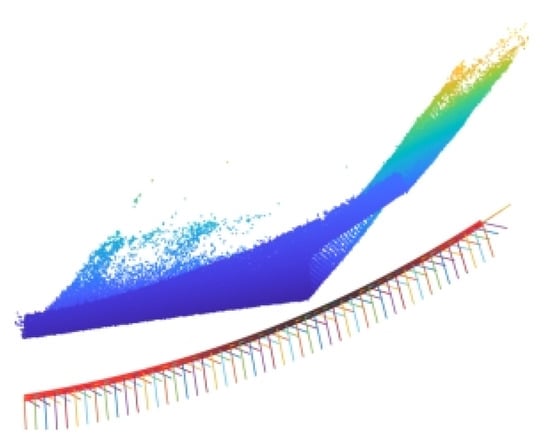
Figure 14.
The performance of the non-cutting path velocity planning.
6.2. Stiffness Identification and Optimization
Figure 15 shows the platform of the stiffness identification. The authors use a tracker to measure the displacements of the end-effector. A tool is designed for the installation of the target ball and force sensor. A bench vise is adopted to load the force.
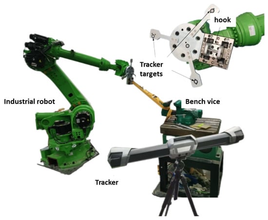
Figure 15.
The platform of the stiffness identification.
According to Section 5, three indices need to be considered, namely the dexterity, and , shown in Figure 16. Three points, denoting three postures, are chosen from the three charts to carry out the identification experiment. The detailed data are partly shown in the Appendix A.
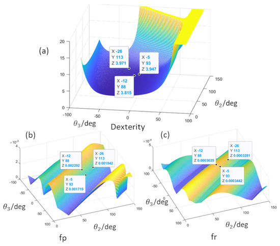
Figure 16.
The platform of the stiffness identification; the calculation results of (a) dexterity, (b) and (c) under and .
The 6D displacement vector can only be solved accurately when the end of the robot is in micro-motion. Only in this case, the relationship formula between the stiffness of the robot joint and the end of the Cartesian stiffness is valid. Therefore, the maximum load during the experiment is set to 200 N.
As the installation location of the sensor does not coincide with tool coordinate system, transformations of the force and torque are necessary. For force, the transformation is:
where is the force data of the sensor, and is the force of the end of the robot. denotes the transformation matrix from the robot to the sensor. For torque, that is:
where denotes the torque on the end of the robot. denotes the distance from the sensor to the end of the robot. denotes the rotation matrix from the end of the robot to the tool coordinate system.
Finally, the least squares method is applied to multiple pairs of force and displacement to improve the accuracy. The detailed data of robot posture configuration and loading are presented in the Appendix A. The joint stiffness of the robot is shown in the following table (Table 2).
Table 2.
The joint stiffness of the robot identification results.
To optimize the angles of the two redundant DOFs of the machining system, the function in (25) is defined as the stiffness evaluation index. Figure 17 shows the result of the traversal simulation of the two redundant DOFs of the machining system using the stiffness evaluation index. Figure 17b is the three-dimensional figure of the simulation result, and Figure 17a is the contour sketch of the right figure. Figure 17c,d is the robot postures before and after optimization. The technological parameters of the milling process: the spindle speed is 6000 r/min, the feed speed is 1 mm/s, the feed is 1mm, and the milling cutter is a 4-blade end mill with a diameter of 10mm. The milling force simulation program and the method of milling force parameter identification refer to the method introduced in [33] for simulation calculation.
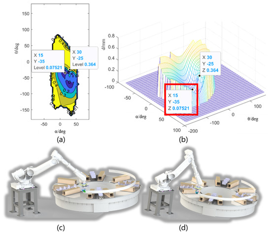
Figure 17.
The result of traversal simulation of the two redundant degrees of freedom. (a) The contour sketch of the displacements; (b) the displacements under all degrees of the two redundant DOFs; (c,d) the robot postures before and after optimization.
6.3. Machining Test
It should be noted that the maximum mean square error of the hand–eye calibration reprojection is 0.41 mm. According to the analysis and optimization results of the processing accuracy in the previous part, the absolute positioning accuracy of the robot improves to be ±0.1 mm by using the hand–eye calibration method. The optimized processing gains the average displacement mode length of the process at 0.07 mm. Considering the above data comprehensively, it is not difficult to find that the machining results cannot meet most of the needs by relying on the absolute positioning accuracy of the robot for milling processing. Therefore, manual tool setting is required before milling to minimize the impact of the absolute positioning accuracy of the robot on the machining accuracy.
For the robot bevel milling process, the comparison effect of the processing result and manual bevel processing are shown in Figure 18. It can be found that the surface quality under visual inspection is similar between robotic milling and manual grinding. The bevel inclination angle needs to be obtained by applying numerical software analysis to the point cloud data after the bevel milling is completed, and the average distance of the blunt edge also needs to be obtained by numerical analysis software. Before evaluating the processing result, the processing requirements are shown in Figure 19.

Figure 18.
Comparison effects of the robot bevel milling processing result and manual bevel processing result.
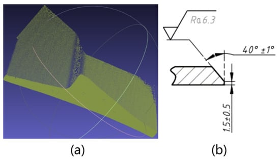
Figure 19.
The evaluation of the processing result. (a) Point cloud data of the milling result; (b) the processing requirements.
The distance between the upper and lower curves on the green plane is the required root size. The result of the distance between the upper and lower edge of the bevel end surface obtained by point cloud data measurement is shown in Figure 20. The basic size is 1.5 mm. The shadow is the tolerance zone in the process requirements. It can be seen that after removing the influence of some error points, the overall indicators are within the process requirements.
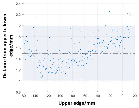
Figure 20.
The distances between the upper and lower edge of the bevel end surface.
Figure 21 is a schematic diagram of calculating the inclination angle of the bevel based on the workpiece point cloud after processing. Nine reference planes are selected equidistantly on the bottom edge curve. Based on numerical analysis software, the bevel angle in each section is analyzed and marked. The error of the angle is under ±1°, which meets the processing requirements.
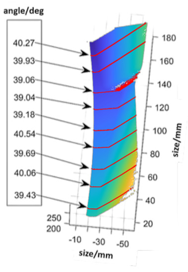
Figure 21.
Schematic diagram of calculating the inclination angle of the bevel based on the workpiece point cloud after processing.
7. Conclusions
In this paper, the authors present a completed work on a robotic milling system. The significance of the work is that it can realize automated robotic milling of low-consistency parts. It liberates workers from the harsh environment and improves the production efficiency.
The main contributions of this paper are as follows:
(1) A hand–eye calibration optimization method is proposed based on GA, which presented a good robustness to system errors.
(2) The authors propose a processing feature extraction method based on the point cloud data of the actual workpiece. The tool paths are generated based on velocity optimization.
(3) A processing posture optimization model based on the robot stiffness is proposed for the specific system with a fixture turntable. The stiffness model ignoring the Kc term is verified by simulation.
(4) The robotic bevel milling task is completed, and the results meet the processing requirements.
In future work, the authors will conduct more process tests to optimize process parameters. The milling path planning method proposed in this paper has good regional adaptability to the different postures of the workpiece, but the robotic milling is not limited to the workpiece involved in this paper. The follow-up should conduct detailed research on the regional features of other parts to improve the adaptability of the tool path planning method.
Author Contributions
Methodology, K.B.; software, K.B.; validation, M.L.; formal analysis, K.B.; investigation, K.B.; resources, Y.G.; data curation, Y.G.; writing—original draft preparation, Y.G.; writing—review and editing, M.L.; supervision, H.G.; project administration, W.D.; funding acquisition, W.D. All authors have read and agreed to the published version of the manuscript.
Funding
This research was funded by the Creative Application Research of China Aerospace Science and Technology (Grant No. A06AB525) and the National Science and Technology Major Project of China (Grant No. 2017ZX04005001-005).
Institutional Review Board Statement
Not applicable.
Informed Consent Statement
Not applicable.
Data Availability Statement
Not applicable.
Conflicts of Interest
The authors declare no conflict of interest.
Appendix A
In this section, the testing data of loading for stiffness identification are partly presented, as shown in Table A1 and Figure A1.
Table A1.
Three postures for loading tests in stiffness identification (unit: deg).
Table A1.
Three postures for loading tests in stiffness identification (unit: deg).
| Posture | AxisI | AxisII | AxisIII | AxisIV | AxisV | AxisVI |
|---|---|---|---|---|---|---|
| 1 | 0 | 93 | −5 | 45 | 45 | 45 |
| 2 | 0 | 113 | −26 | 45 | 45 | 45 |
| 3 | 0 | 88 | −12 | 45 | 45 | 45 |
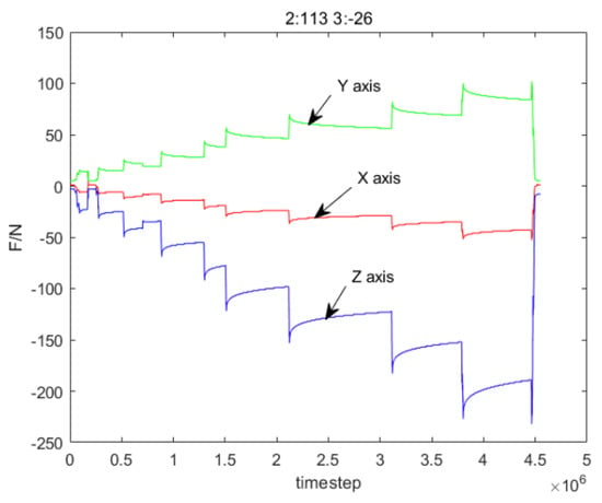
Figure A1.
The recorded data of the force sensor during several loadings of Posture 2.
References
- Lei, P.; Zheng, L.; Xiao, W.; Li, C.; Wang, D. A closed-loop machining system for assembly interfaces of large-scale component based on extended STEP-NC. Int. J. Adv. Manuf. Technol. 2017, 91, 2499–2525. [Google Scholar] [CrossRef]
- Moeller, C.; Schmidt, H.C.; Koch, P.; Boehlmann, C.; Kothe, S.; Wollnack, J.; Hintze, W. Real Time Pose Control of an Industrial Robotic System for Machining of Large Scale Components in Aerospace Industry Using Laser Tracker System. SAE Int. J. Aerosp. 2017, 10, 100–108. [Google Scholar] [CrossRef] [Green Version]
- Chen, Y.; Dong, F. Robot machining: Recent development and future research issues. Int. J. Adv. Manuf. Technol. 2013, 66, 1489–1497. [Google Scholar] [CrossRef] [Green Version]
- Qin, C.; Tao, J.; Wang, M.; Liu, C. A novel approach for the acquisition of vibration signals of the end effector in robotic drilling. In Proceedings of the 2016 IEEE International Conference on Aircraft Utility Systems (AUS), Beijing, China, 10–12 October 2016; pp. 522–526. [Google Scholar]
- Pham, A.D.; Ahn, H.J. High Precision Reducers for Industrial Robots Driving 4th Industrial Revolution: State of Arts, Analysis, Design, Performance Evaluation and Perspective. Int. J. Precis. Eng. Manuf.-Green Technol. 2018, 5, 519–533. [Google Scholar] [CrossRef]
- Cordes, M.; Hintze, W.; Altintas, Y. Chatter stability in robotic milling. Robot. Comput.-Integr. Manuf. 2019, 55, 11–18. [Google Scholar] [CrossRef]
- He, F.x.; Liu, Y.; Liu, K. A chatter-free path optimization algorithm based on stiffness orientation method for robotic milling. Int. J. Adv. Manuf. Technol. 2019, 101, 2739–2750. [Google Scholar] [CrossRef]
- Safi, S.M.; Amirabadi, H.; Lirabi, I.; Khalili, K.; Rahnama, S. A new Approach for Chatter Prediction in Robotic milling Based on Signal Processing in Time domain. Appl. Mech. Mater. 2013, 346, 45–51. [Google Scholar] [CrossRef]
- Leonesio, M.; Villagrossi, E.; Beschi, M.; Marini, A.; Bianchi, G.; Pedrocchi, N.; Tosatti, L.M.; Grechishnikov, V.; Ilyukhin, Y.; Isaev, A. Vibration Analysis of Robotic Milling Tasks. Procedia CIRP 2018, 67, 262–267. [Google Scholar] [CrossRef]
- Kuss, A.; Drust, M.; Verl, A. Detection of Workpiece Shape Deviations for Tool Path Adaptation in Robotic Deburring Systems. Procedia CIRP 2016, 57, 545–550. [Google Scholar] [CrossRef]
- Han, L.; Cheng, X.; Li, Z.; Zhong, K.; Shi, Y.; Jiang, H. A robot-driven 3D shape measurement system for automatic quality inspection of thermal objects on a forging production line. Sensors 2018, 18, 4368. [Google Scholar] [CrossRef] [Green Version]
- Yu, C.; Chen, X.; Xi, J. Modeling and calibration of a novel one-mirror galvanometric laser scanner. Sensors 2017, 17, 164. [Google Scholar] [CrossRef] [Green Version]
- Wang, J.; Tao, B.; Gong, Z.; Yu, S.; Yin, Z. A Mobile Robotic Measurement System for Large-scale Complex Components Based on Optical Scanning and Visual Tracking. Robot. Comput.-Integr. Manuf. 2020, 67, 102010. [Google Scholar] [CrossRef]
- Ge, J.; Deng, Z.; Li, Z.; Li, W.; Lv, L.; Liu, T. Robot welding seam online grinding system based on laser vision guidance. Int. J. Adv. Manuf. Technol. 2021, 116, 1737–1749. [Google Scholar] [CrossRef]
- Guo, W.; Zhu, Y.; He, X. A Robotic Grinding Motion Planning Methodology for a Novel Automatic Seam Bead Grinding Robot Manipulator. IEEE Access 2020, 8, 75288–75302. [Google Scholar] [CrossRef]
- Yin, S.; Ren, Y.; Guo, Y.; Zhu, J.; Yang, S.; Ye, S. Development and calibration of an integrated 3D scanning system for high-accuracy large-scale metrology. Measurement 2014, 54, 65–76. [Google Scholar] [CrossRef]
- Xu, X.; Zhu, D.; Zhang, H.; Yan, S.; Ding, H. TCP-based calibration in robot-assisted belt grinding of aero-engine blades using scanner measurements. Int. J. Adv. Manuf. Technol. 2017, 90, 635–647. [Google Scholar] [CrossRef]
- Wu, D.; Chen, T.; Li, A. A high precision approach to calibrate a structured light vision sensor in a robot-based three-dimensional measurement system. Sensors 2016, 16, 1388. [Google Scholar] [CrossRef] [PubMed]
- Niola, V.; Rossi, C.; Savino, S.; Strano, S. A method for the calibration of a 3-D laser scanner. Robot. Comput.-Integr. Manuf. 2011, 27, 479–484. [Google Scholar] [CrossRef]
- Chen, W.; Du, J.; Xiong, W.; Wang, Y.; Chia, S.; Liu, B.; Cheng, J.; Gu, Y. A Noise-Tolerant Algorithm for Robot-Sensor Calibration Using a Planar Disk of Arbitrary 3-D Orientation. IEEE Trans. Autom. Sci. Eng. 2018, 15, 251–263. [Google Scholar] [CrossRef]
- Yin, S.; Ren, Y.; Zhu, J.; Yang, S.; Ye, S. A vision-based self-calibration method for robotic visual inspection systems. Sensors 2013, 13, 16565–16582. [Google Scholar] [CrossRef] [Green Version]
- Santolaria, J.; Aguilar, J.J.; Guillomía, D.; Cajal, C. A crenellated-target-based calibration method for laser triangulation sensors integration in articulated measurement arms. Robot. Comput.-Integr. Manuf. 2011, 27, 282–291. [Google Scholar] [CrossRef]
- Carlson, F.B.; Johansson, R.; Robertsson, A. Six DOF eye-to-hand calibration from 2D measurements using planar constraints. In Proceedings of the 2015 IEEE/RSJ International Conference on Intelligent Robots and Systems (IROS), Hamburg, Germany, 28 September–2 October 2015; pp. 3628–3632. [Google Scholar] [CrossRef] [Green Version]
- Sharifzadeh, S.; Biro, I.; Kinnell, P. Robust hand-eye calibration of 2D laser sensors using a single-plane calibration artefact. Robot. Comput.-Integr. Manuf. 2020, 61, 101823. [Google Scholar] [CrossRef]
- Kim, S.H.; Nam, E.; Ha, T.I.; Hwang, S.H.; Lee, J.H.; Park, S.H.; Min, B.K. Robotic Machining: A Review of Recent Progress. Int. J. Precis. Eng. Manuf. 2019, 20, 1629–1642. [Google Scholar] [CrossRef]
- Nubiola, A.; Bonev, I.A. Absolute calibration of an ABB IRB 1600 robot using a laser tracker. Robot. Comput.-Integr. Manuf. 2013, 29, 236–245. [Google Scholar] [CrossRef]
- Dumas, C.; Caro, S.; Cherif, M.; Garnier, S.; Furet, B. Joint stiffness identification of industrial serial robots. Robotica 2012, 30, 649–659. [Google Scholar] [CrossRef] [Green Version]
- Klimchik, A.; Pashkevich, A.; Chablat, D. CAD-based approach for identification of elasto-static parameters of robotic manipulators. Finite Elem. Anal. Des. 2013, 75, 19–30. [Google Scholar] [CrossRef] [Green Version]
- Huang, T.; Zhao, X.; Whitehouse, D.J. Stiffness estimation of a tripod-based parallel kinematic machine. IEEE Trans. Robot. Autom. 2002, 18, 50–58. [Google Scholar] [CrossRef]
- Deblaise, D.; Hernot, X.; Maurine, P. A systematic analytical method for PKM stiffness matrix calculation. In Proceedings of the Proceedings 2006 IEEE International Conference on Robotics and Automation, Orlando, FL, USA, 15–19 May 2006; pp. 4213–4219. [Google Scholar] [CrossRef]
- Gong, C.; Yuan, J.; Ni, J. Nongeometric error identification and compensation for robotic system by inverse calibration. Int. J. Mach. Tools Manuf. 2000, 40, 2119–2137. [Google Scholar] [CrossRef]
- Jang, J.H.; Kim, S.H.; Kwak, Y.K. Calibration of geometric and non-geometric errors of an industrial robot. Robotica 2001, 19, 311–321. [Google Scholar] [CrossRef] [Green Version]
- Altintas, Y.; Ber, A. Manufacturing Automation: Metal Cutting Mechanics, Machine Tool Vibrations, and CNC Design. Appl. Mech. Rev. 2001, 54, B84. [Google Scholar] [CrossRef]
- Khalil, W.; Besnard, S. Geometric calibration of robots with flexible joints and links. J. Intell. Robot. Syst. Theory Appl. 2002, 34, 357–379. [Google Scholar] [CrossRef]
- Salisbury, J.K. Active Stiffness Control of a Manipulator in Cartesian Coordinates. In Proceedings of the 1980 19th IEEE Conference on Decision and Control including the Symposium on Adaptive Processes, Albuquerque, NM, USA, 10–12 December 1980; Volume 1, pp. 95–100. [Google Scholar] [CrossRef]
- Chen, S.F. The 6 × 6 stiffness formulation and transformation of serial manipulators via the CCT theory. In Proceedings of the 2003 IEEE International Conference on Robotics and Automation (Cat. No.03CH37422), Taipei, Taiwan, 14–19 September 2003; Volume 3, pp. 4042–4047. [Google Scholar] [CrossRef]
- Chen, S.F.; Kao, I. Conservative congruence transformation for joint and Cartesian stiffness matrices of robotic hands and fingers. Int. J. Robot. Res. 2000, 19, 835–847. [Google Scholar] [CrossRef]
Publisher’s Note: MDPI stays neutral with regard to jurisdictional claims in published maps and institutional affiliations. |
© 2021 by the authors. Licensee MDPI, Basel, Switzerland. This article is an open access article distributed under the terms and conditions of the Creative Commons Attribution (CC BY) license (https://creativecommons.org/licenses/by/4.0/).