Abstract
In order to solve the problems of repetitive and non-repetitive interference in the workflow of Automated Guided Vehicle (AGV), Iterative Learning Control (ILC) combined with linear extended state observer (LESO) is utilized to improve the control accuracy of AGV drive motor. Considering the working conditions of AGV, the load characteristics of the drive motor are analyzed with which the mathematical model of motor system is established. Then the third-order extended state space equations of the system approximate model is obtained, in which LESO is designed to estimate the system states and the total disturbance. For the repeatability of AGV workflow, ILC is designed to improve the control accuracy. As the goods mass transported each time is not same, the LESO is utilized to estimate the non-repetitive load disturbance in real time and compensate the disturbance of the system to improve the position precision. The convergence of the combined algorithm is also verified. Simulation and experimental results show that the proposed iterative learning control strategy based on LESO can reduce the positioning error in AGV workflow and improve the system performance.
1. Introduction
In order to shorten the processing cycle and reduce production costs, it is necessary to develop intelligent logistics equipment vigorously [1]. In recent years, automated guided vehicle (AGV) technology has been widely developed. The workflow of AGV is repetitive: when AGV has planned the route, it will continue to move the goods from the loading point to the transfer point along the designed route until all of the materials are transported. However, the weight of goods (such as express delivery) is not necessarily consistent which will lead to non-repetition of AGV workflow. For the friction between the wheel and the ground is the main load of the AGV, and the friction has strong nonlinear at low speed, AGV is needed to keep steady in loading or transferring process. So the motor system is required with high precision, fast response and strong anti-interference control performance. Traditional PID control can not have high control performance for variable load [2], so it is significance to research the high-performance control strategy of AGV drive motor servo system according to the working conditions to improve the positioning accuracy and logistics efficiency.
ILC was first proposed by Uchiyama in 1978. According to the existing repeated tracking information, ILC achieves zero error tracking along the desired trajectory in a finite time interval. ILC has no requirement for the accurate mathematical model of the system, does not need to identify the system parameters, and has strong adaptability to nonlinear and uncertain systems [3,4,5]. However, ILC can’t effectively deal with these problems in the presence of non-repeatability and random disturbance/noise [6]. Therefore, ILC often needs to integrate other advanced control methods to achieve the desired control effect.
In reference [7], ILC can’t achieve ideal control effect in incomplete repetitive scenarios. To solve this problem, ILC and disturbance observer (DOB) are combined to compensate non-repetitive disturbances in repetitive tasks. As the core of Active Disturbance Rejection Control [8], LESO can estimate and compensate for internal and external disturbances, improving the robustness of the system, playing a similar role to DOB. In reference [9], the influence of periodic interference and random measurement noise on the tracking accuracy of the system is suppressed by adaptive learning gain. In order to reduce the noise and other disturbances in the feedback channel, a control strategy combining iterative learning with FIR filter is proposed in reference [10], which improves the anti-interference ability of the system. In order to suppress the torque ripple of switched reluctance motor, the linear iterative extended state observer in the iterative domain was used to compensate the uncertainty in the periodic process [11]. Aiming at the nonlinear systems with time delay, reference [12] combines the initial state iterative learning law with the input iterative learning law, and relaxes the convergence condition of the iterative learning control algorithm. According to the running state of AGV drive motor, particle swarm optimization algorithm [13] is used to adjust the parameters of fuzzy control in real time to improve the stability of AGV.
This paper takes AGV drive servo system as the research object, establish the third-order expansion equation of the system. The operation of AGV is full of a lot of repetitive information but it is not used, and there are some restrictions on the use of iterative learning control, So an ILC strategy based on LESO is designed for this situation. The disturbance is estimated and compensated by LESO, and the baseline error is reduced to an acceptable range. Through continuous iteration, the repetition is compensated. It can further improve the tracking accuracy. Simulations and experiments show that this control strategy can effectively compensate for the repetitive and non-repetitive interference in AGV drive servo system.
2. Mathematical Model of AGV Drive Servo System
The load on the AGV drive motor is mainly from the friction between the ground and the wheels. Coulomb friction model [14] is used in this paper, and it can be constructed as
where, Ff is the friction force received by the wheel; Ft is the driving force transmitted by the motor to the wheel; Fm is the maximum static friction force between the wheel and the ground. The rolling friction force is considered to be equal to the maximum static friction force.
Then the load torque expression at the motor side is
where, M is the mass of the cargo; m is the mass of the AGV itself; g is the acceleration due to gravity; f is the friction coefficient between the wheel and the ground; r is the radius of the driving wheel; i is the reduction ratio of the reducer.
The relationship between the magnitude of friction and speed is strong nonlinear. Friction will have a greater impact on the positioning accuracy of AGV drive servo system, especially when motor is running slowly, it will have influence on the stability of AGV drive servo system.
This article mainly focused on small load AGV because of its wide application. The wheel material is polyurethane and the workshop floor uses epoxy floor paint. Take the small AGV model MiR250 as example, its parameters are shown in Table 1.

Table 1.
Parameter table of AGV.
After calculating with the data in the Table 1, the torque when the AGV is unloaded is Tf1 = 0.122 N·m, the torque When the AGV is fully loaded is Tf2 = 0.490 N·m.
When AGV is in the rated working condition, the power and speed of the driving motor are
AGV drive servo system mainly consists of DC servo motor, drive controller, wheel, gearbox [15], etc. A permanent magnet synchronous motor (PMSM) of 200 W was selected in this paper. The parameters table of the selected motor are shown in Table 2.
Table 2.
Parameter table of PMSM.
The mathematical model of the PMSM is [16]
where, ud, uq are motor d, q axis stator voltage; id, iq are motor d, q axis stator current;
The system torque equation is [17]
Te is the motor electromagnetic torque; θm is the motor angular displacement; θ is the system angular displacement.
Ignore the armature inductance Ls, treat the current loop and the speed loop as open loops, and use the vector control method with id = 0. In this case, the system model is established, as shown in Figure 1.

Figure 1.
Drive servo system of AGV.
Figure 1.
Drive servo system of AGV.
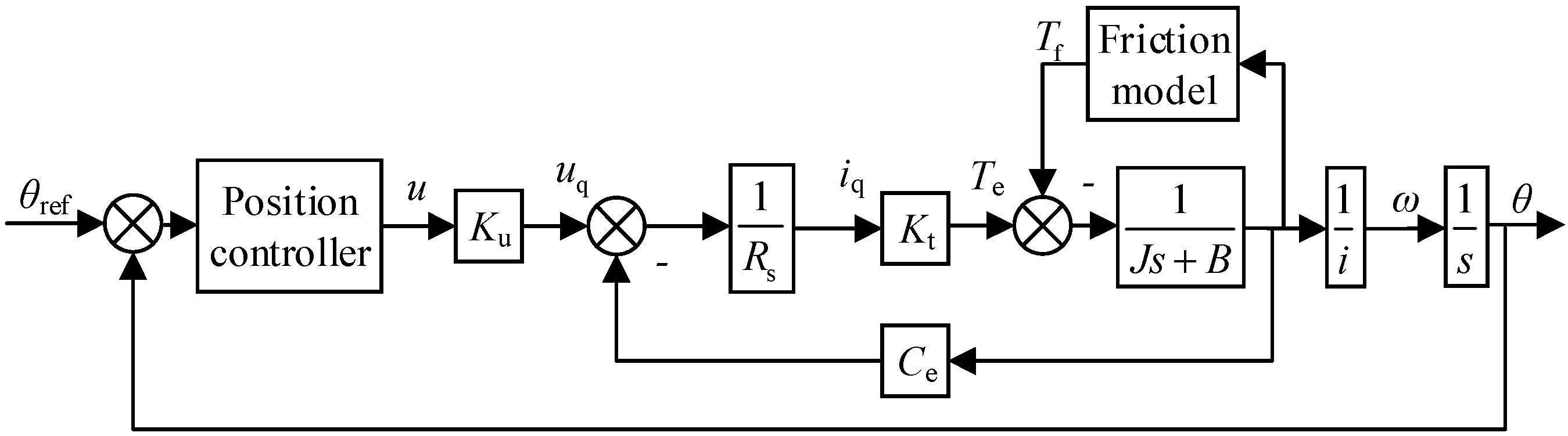
On this basis, the dynamic equation of the PMSM control system is established.
set as a, as b, Convert Equation (7) to state equation
where, x1 is the system angular displacement; x2 is the system angular velocity.
Establish three loops (position loop, speed loop and current loop) control model of AGV drive servo system, as shown in Figure 2.
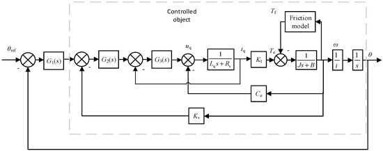
Figure 2.
Drive servo system model of AGV.
In the figure, G1(s), G2(s) and G3(s) are the controller transfer functions of the position loop, speed loop and current loop respectively; Kv is the speed feedback coefficient.
3. Design of Iterative Learning Controller Based on LESO
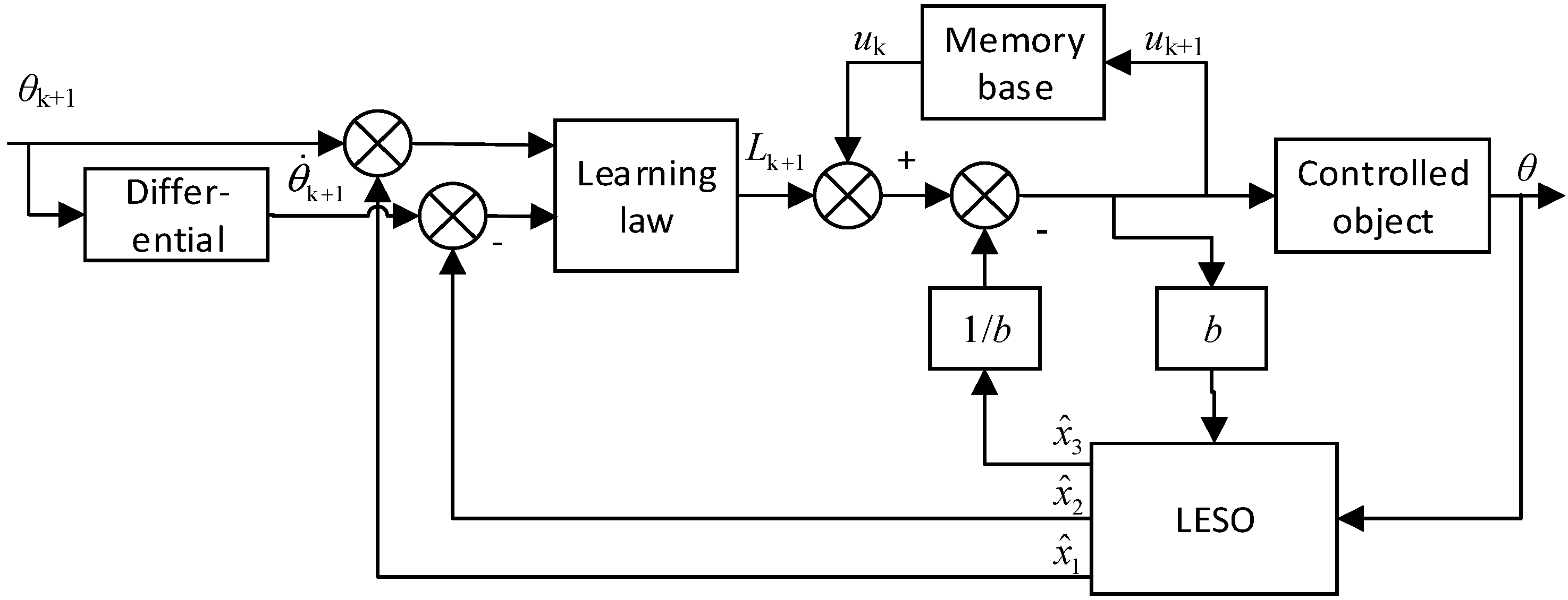
The inner loop model of AGV drive servo system is used as the controlled object, and the outer loop position controller adopts iterative learning control combined with active disturbance rejection technology to improve the accuracy of the AGV’s repeated operation and enhance the anti-interference against non-repetitive disturbances ability. The controller mainly includes iterative learning controller and linear expansion state observer. Its overall block diagram is shown as in Figure 3.
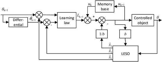
Figure 3.
Block diagram of Iterative learning control based on LESO.
3.1. Iterative Learning Controller
Iterative learning control is suitable for repetitive running systems. This paper adopts the closed-loop PD learning law [18]. Its structure is as follows
where, uk+1(t) is the control quantity of the k + 1th iteration at time t; uk(t) is the control quantity of the kth iteration at time t; yd(t) is the desired trajectory; yk+1 (t) is the output of the k + 1 iteration at time t; Kp and Kd are the proportional and differential coefficients, respectively.
Since the prerequisite for applying ILC is that the system is repeatable, this requires the system to meet the following assumptions:
- (1)
- Specify the desired trajectory in advance;
- (2)
- The initial state before each iteration is the same;
- (3)
- Each iteration, the output of the system is measurable;
- (4)
- The time interval for each operation of the system is limited and fixed, namely t ∈ [0,T];
- (5)
- There is a unique ideal control input ud(t) make the actual state and actual output of the system be the desired state and ideal output respectively.
3.2. Linear Extended State Observer
Take the unknown part of the system state Equation (8) as x3, and write the original state equation into the following expanded state form
where, g(x,Tf) is the derivative of Δ; Δ is the total disturbance of the servo system, and Δ is bounded.
In order to better observe the position, speed, and unknown part of the system, an extended state observer is used to compensate for the unknown uncertainty and external interference. The parameters of the linear extended state observer [19] (LESO) proposed based on the system bandwidth theory are easier to adjust. Its structure [20] is as follows
where, is the estimated value of position output; is the estimated value of speed output; is the estimated value of total disturbance; is LESO bandwidth.
3.3. Iterative Learning Controller Based on LESO
From Equation (10), the state equation of AGV drive servo system can be obtained as
among them, x(t) = [x1(t), x2(t), x3(t)]T, B = [0,b,0]T, C = [0,0,1].
Then the iterative learning control law based on LESO is
where, , is the estimate of x.
Lemma 1 [21] If operator Satisfy
where M and q are non-negative constants, the following conclusions can be drawn
- (1)
- ∀y ∈ Cr[0,T] has a unique x ∈ Cr[0,T] make
- (2)
- Define operatorwhere x ∈ Cr[0,T] is the only solution defined by 1. Then there is M1 > 0, make
Lemma 2 [21] Set constant sequence {bk}k>0 (bk ≥ 0) Converge to zero, operator
where M > 0, Cr[0,T] is the r-dimensional vector taking the maximum norm, and Q(t) is the r * r-dimensional continuous matrix, let Q:Cr[0,T] → Cr[0,T] is
If the spectral radius of Q is less than 1,
consistently holds for t.
The convergence analysis of the control law proposed in the article is as follows:
The error of the kth iteration can be expressed as
xd(t), yd(t), ud(t) is the state, output and control on the desired trajectory respectively.
Let , then
Differentiate δyk+1(t)
Therefore
Define as
Let Equation (25) can be written as
Combined with Equation (23), it can be obtained
According to the Bellman-Gronwall theorem [22], there exists M1 > 0, which satisfies
Let
where , is the initial state of the system , The solution when the control quantity u takes u and v, so
Take its norm after integration
f(t, x) satisfies Lipschiz condition [23] for x
So exist M2 > 0
Similarly, there exists , so that
From Lemma 1, there is makes Equation (27) satisfy the follow equation
where satisfy
Define
There is , making also satisfies Equation (38), so Equation (37) can be written as
From lemma 2, when the spectral radius of ρ[(I + KdCB)−1] is less than 1, then is consistent. When Kd > 0, the error of AGV servo system converges gradually after iteration.
4. Simulation Analysis
This article takes AGV drive servo system as the object, establishes the permanent magnet synchronous motor simulation model in the Matlab/Simulink environment based on the data in Table 1. According to the aforementioned Coulomb friction model, the simulation model of AGV drive servo system is established.
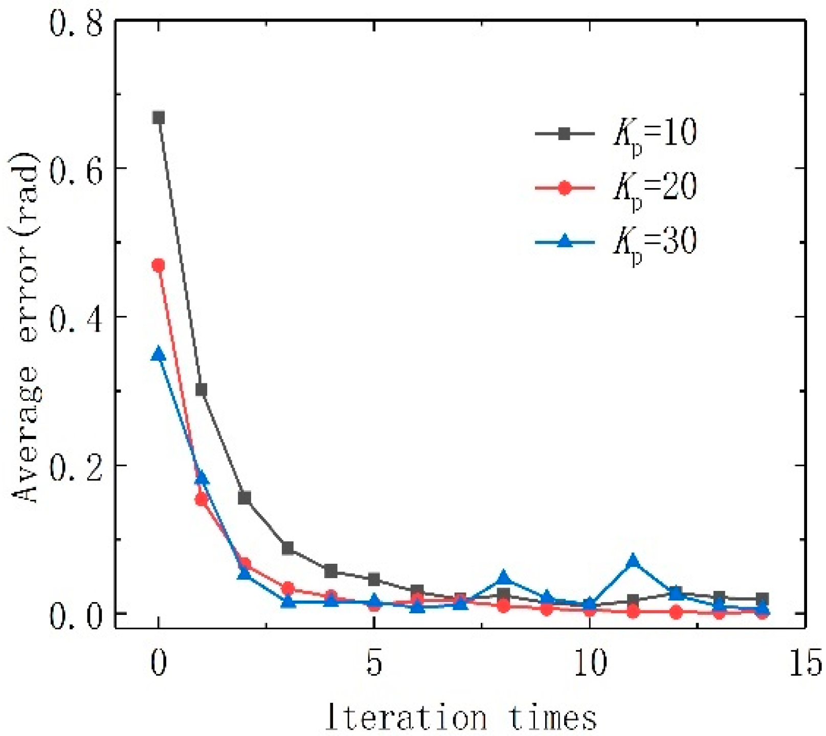
The control parameters of LESO+ILC mainly include the parameters Kp and Kd of the PD-type iterative control law and the bandwidth ωo of the linear extended state observer. The influence of these parameters on the control effect. Target curve is θref = 2sin(t). In order to facilitate observation, the average value of tracking error after each iteration is drawn as Figure 4, Figure 5 and Figure 6. They mainly show the impact of different parameter changes on the speed and robustness of iteration.
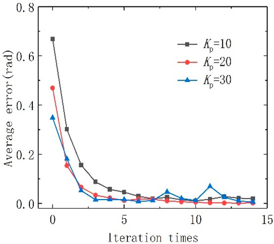
Figure 4.
Error convergence curve of different Kp.
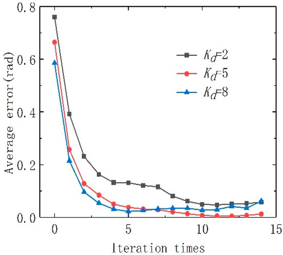
Figure 5.
Error convergence curve of different Kd.
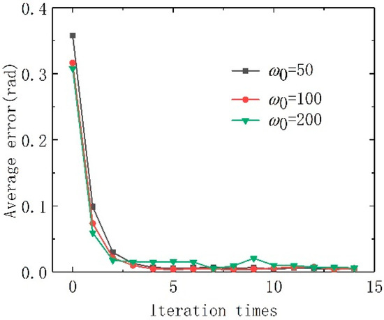
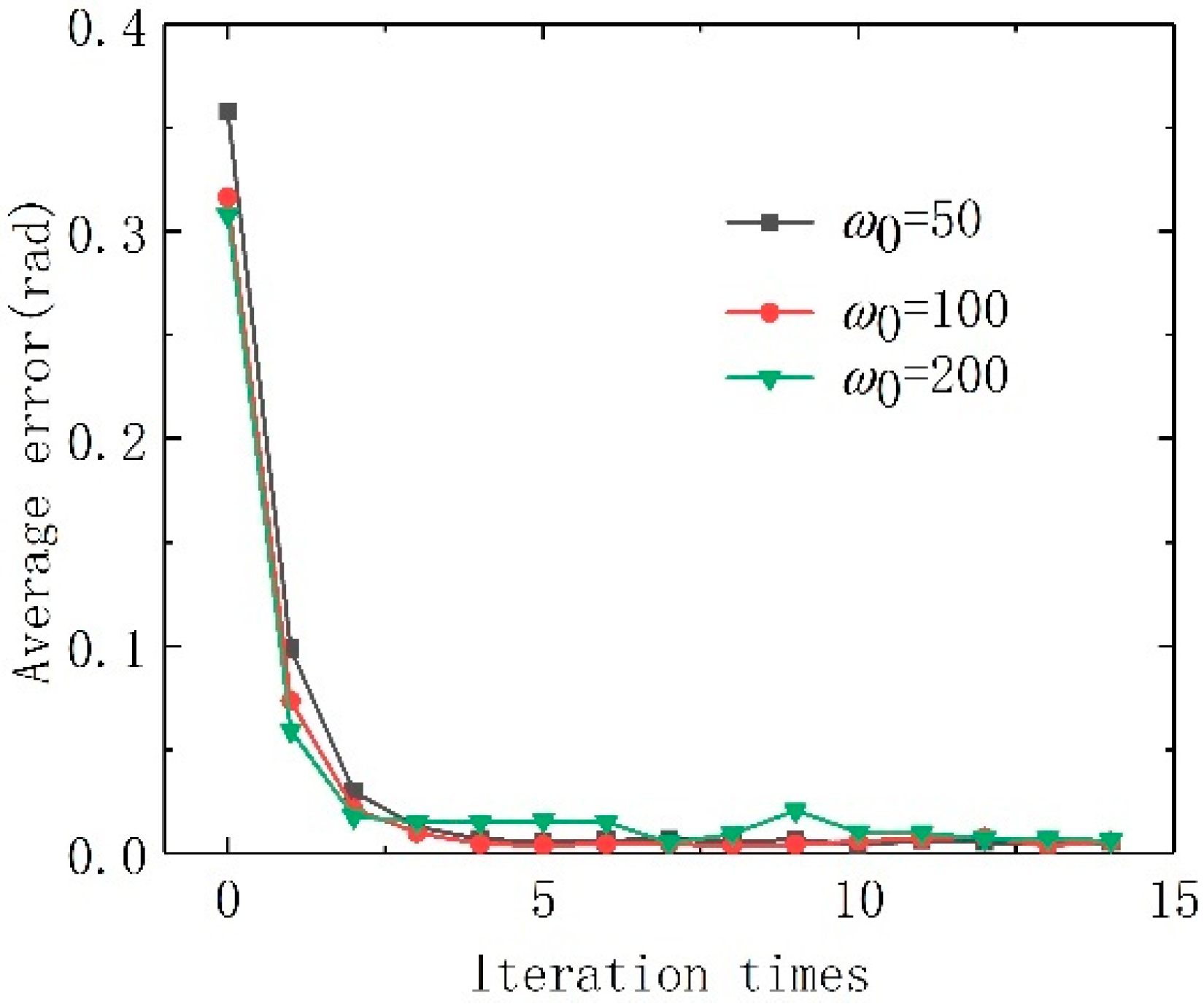
Figure 6.
Error convergence curve of different bandwidths.
Figure 4 shows that when Kp increases, the error of the first iteration will decrease and the error will converge faster, but when Kp is too large, the error is more susceptible to fluctuations. Finally Kp is taken as 20.
Figure 5 shows that the convergence speed of the error is not fast enough when Kd is too small. When Kd is too large, the fluctuation range will be large after stable, and may even diverge. After debugging, Kd is taken as 5.
Figure 6 shows that the larger the LESO bandwidth ωo, the better the compensation effect of the system, and the faster the iterative error converges with the iterative process. The ωo should not be too large, and finally ωo = 100.
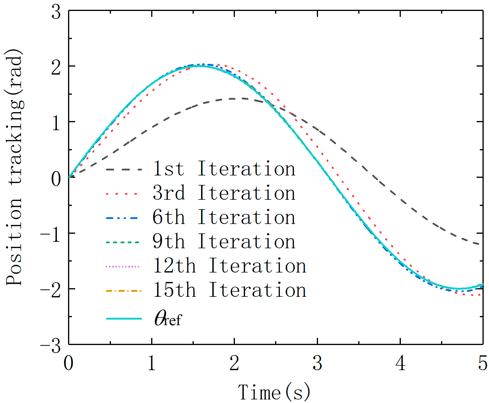
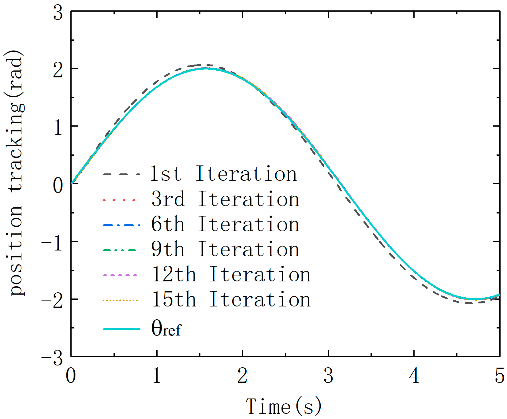
Given signal θref = 2sin(t) rad. The friction force in each iteration is set to a random value between 0.12 and 0.49 N·m. The simulation results of ILC and LESO+ILC algorithms are shown in Figure 7 and Figure 8.
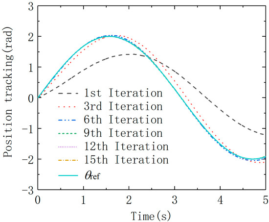
Figure 7.
Position tracking curves based on ILC.
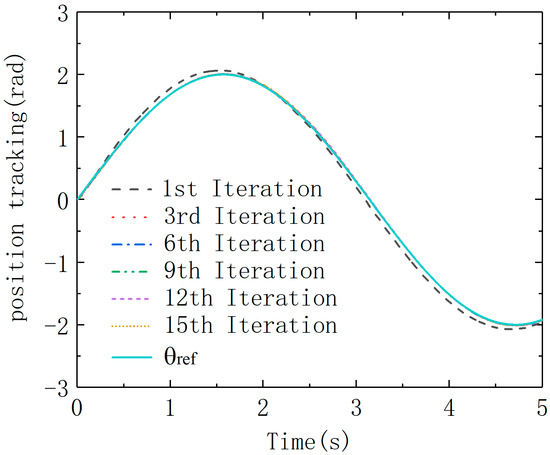
Figure 8.
Position tracking curves based on LESO+ILC.
Figure 7 shows that there is a large gap between the position tracking curve and the given curve in the first iteration of the ILC. After several iterations, the position error continues to decrease. After 9 iterations, the error has basically achieved convergence. It can be seen from Figure 8 that when LESO+ILC is used, the initial error with iteration is significantly reduced while the time required for error convergence is reduced. The robustness of the system with non-repetitive interference is improved.
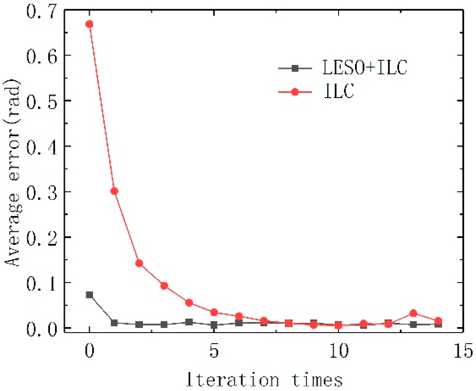
From the iterative error curve Figure 9, it can be seen that the iterative learning control algorithm based on LESO speeds up the speed of the system iterative error convergence, and the error fluctuation after convergence is smaller. Therefore, this algorithm can improve the system’s ability to suppress non-repetitive disturbances and relax the restrictions on the use of ILC.
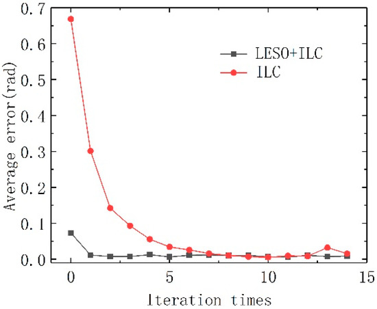
Figure 9.
Iterative error curves.
5. Experiment Verification
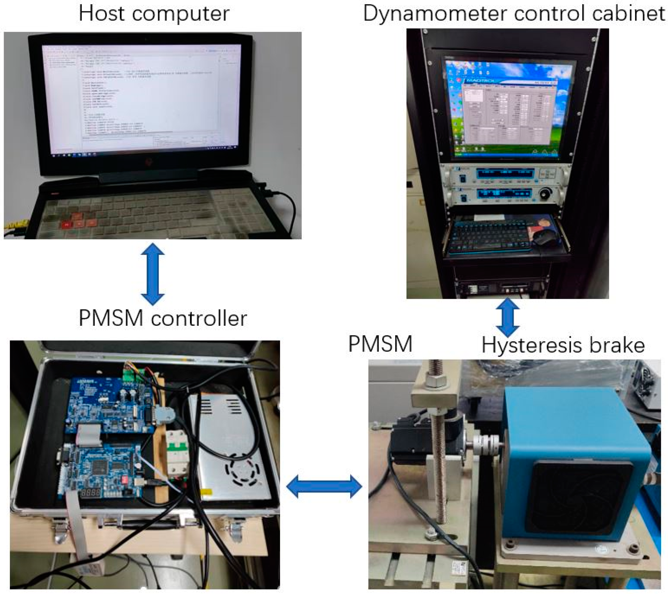
AGV drive servo system experiment platform is mainly composed of a PMSM, a controller, an intelligent power module (IPM), a host computer, and a dynamometer, and its overall structure is shown in Figure 10.

Figure 10.
Experimental platform.
The motor is fixed by a bracket and connected to the dynamometer through a coupling. The dynamometer sets the output torque according to the load. The brand of the dynamometer is MEGTROL, and it consists of a hysteresis brake (which model is HD-510-8NA-0100) and a control cabinet. The control cabinet mainly integrates excitation current controller DSP6001 and power analyzer DSP6530. The torque of MEGTROL is directly related to the excitation current and independent of the motor speed, which is similar to the nature of friction. The encoder feeds back the rotor position of the motor to the controller to meet the needs of vector control. The model of the PMSM we used is MIGE:60CSTMOO630. The motor controller chip model is DSP-TMS320f28335, and the control program is completed in its supporting software CCS9.0.1. The controller generates the corresponding control quantity, controls the IPM output current through SVPWM(Space Vector Pulse Width Modulation) technology, and completes the control of the motor. The experimental platform is shown in the Figure 10.
The given signal is θref = 2πsin(2t) rad, and the load is set according to the conditions in the simulation. The AGV is always in the loading and unloading state, so the torque borne by the motor is between 0.12 (unload) and 0.49 (rated load) N·m. The random disturbance of AGV is the model uncertainties with different load torque, so three load cases (rated load, half load and no-load) are taken in the experiment to verify the controller effectiveness.
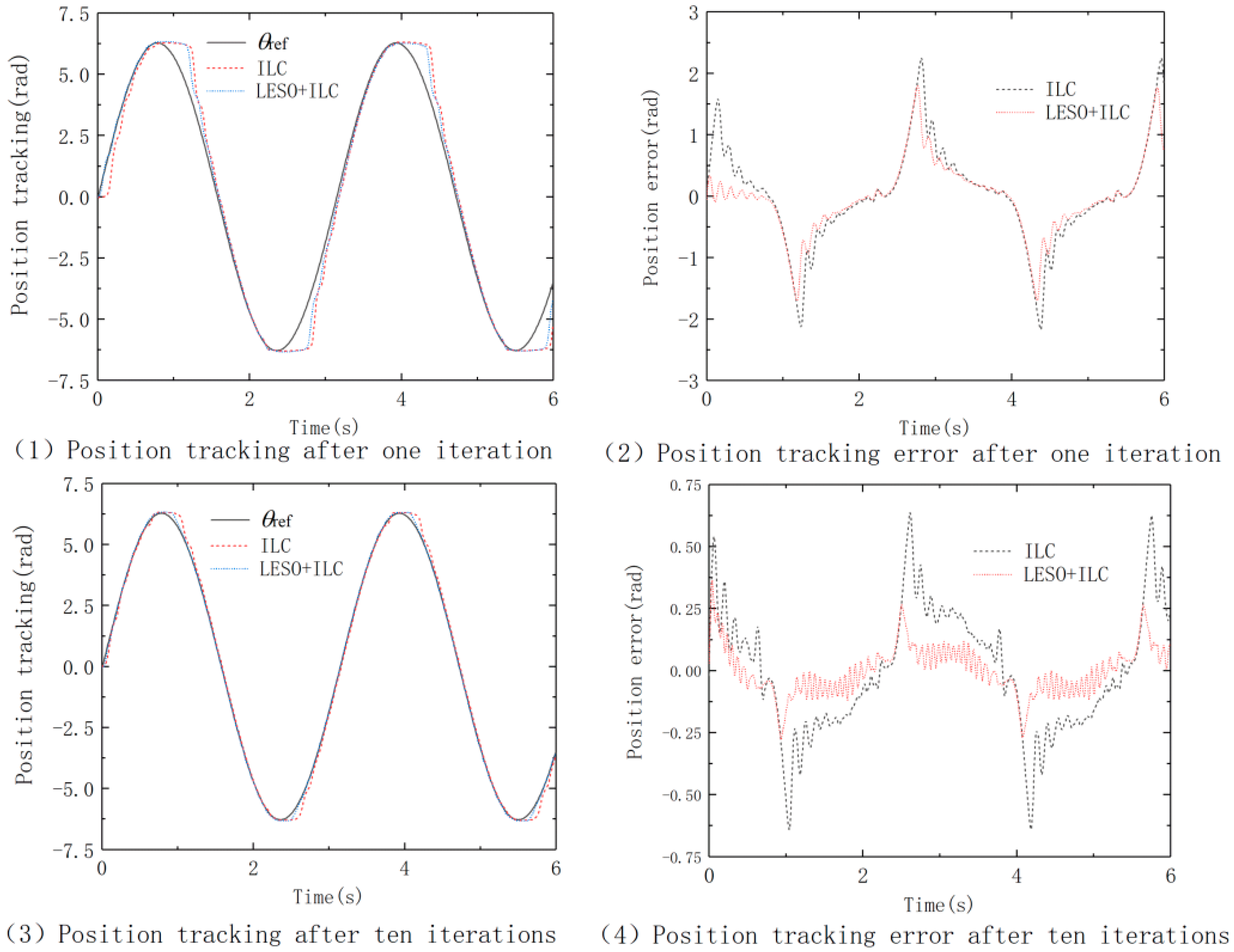
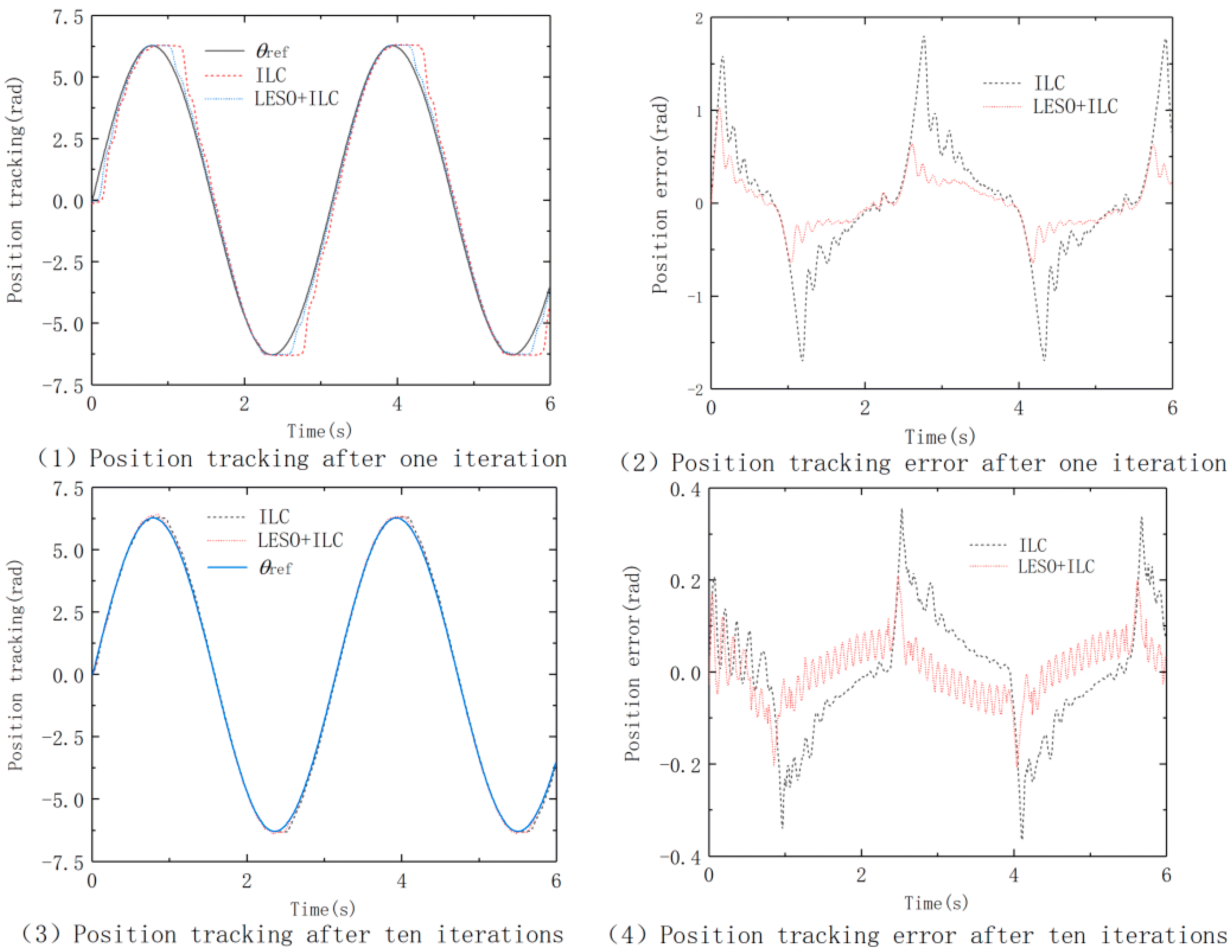
The position tracking curves of rated load are shown in Figure 11. It can be seen from subfigures (1,2) that the tracking curve of ILC and LESO+ILC with bigger error at the peaks and troughs after one iteration. This is because when the motor rotor turns here, the motor stops and the motor output torque is zero. When the motor needs to rotate, the output torque gradually increases until it is greater than the friction torque applied by the dynamometer before the motor starts to run. LESO can compensate external disturbance to improve tracking performance, reducing tracking error.
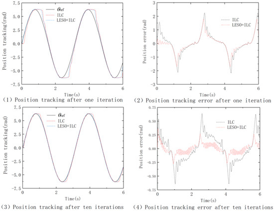
Figure 11.
Position tracking and error curve with rated load.
Subfigures (3,4) indicate the position tracking after ten iterations. Compared with subfigures (1,2), it can be seen that the overall tracking error is reduced after iteration. Due to the characteristics of the load and the limitation of the output current, the error of the curve at the peak and trough can not be completely eliminated, but it is also deceased.
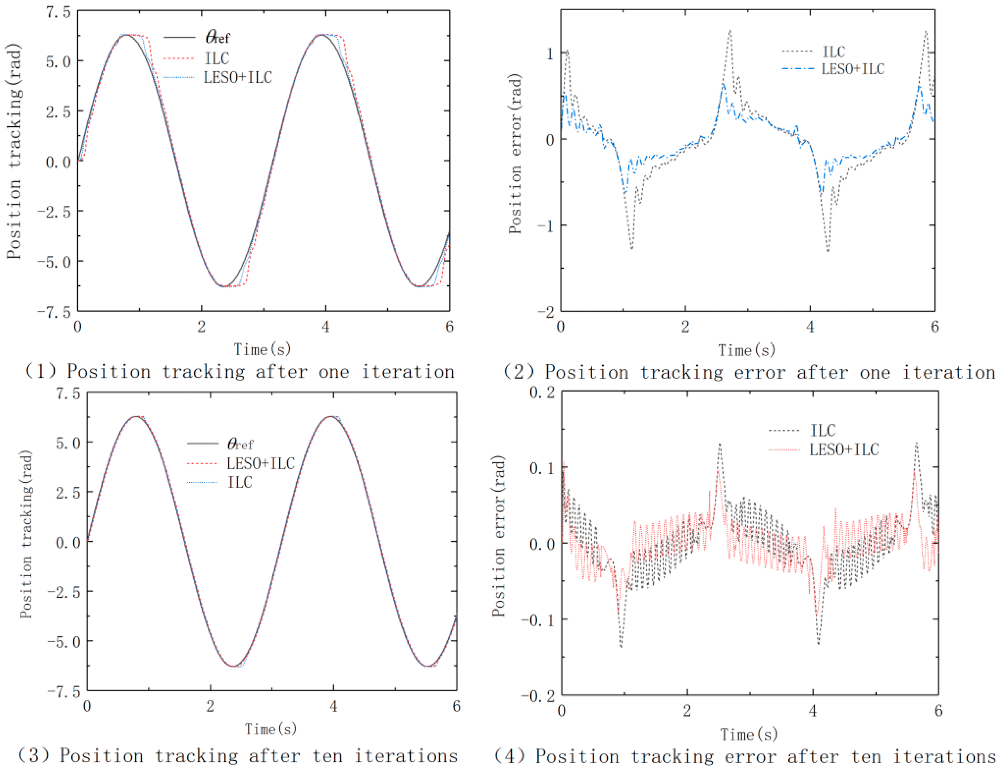
When AGV is in the state of half load (half load is 0.3 N·m), the position tracking of different algorithms is shown in Figure 12.
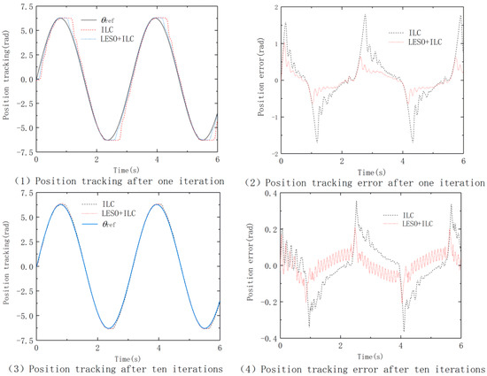
Figure 12.
Position tracking and error curve with half load.
Similarly, the maximum error occurs when the speed approaches zero, but it is reduced compared with the rated load. The position tracking error get convergence to a certain extent due to the iterative algorithm with the disturbance and uncertainties observed and compensated by LESO, the proposed controller LESO+ILC has better tracking performance.
When AGV is in the state of unload, the position tracking of the two algorithms is shown in Figure 13.
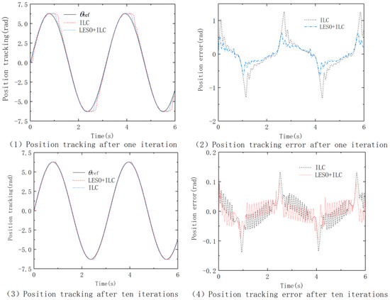
Figure 13.
Position tracking and error curve without load.
After one iteration, compared with the situation of rated load and half load, we can see that with the decrease of load, the maximum error and average error of position tracking also decrease, but LESO+ILC is smaller than ILC.
From subfigures (3,4), we can obtain ILC can reduced tracking error in the iterative process, and LESO+ILC have a better control performance than ILC. Compared with the rated load, the regulation time of the motor at the peak and trough is shortened.
From the above analysis, it can be concluded that the tracking error is reduced after iteration and the error of LESO+ILC is smaller than that of ILC. The regulating time is of LESO+ILC is less than that of ILC. This proves that LESO can estimate and compensate the disturbance to improve the tracking performance.
6. Conclusions
In this paper, an iterative learning control algorithm based on LESO is proposed to solve the problem of the coexistence of repetitive and non-repetitive disturbances in AGV, and the stability of the system is proved. The simulation and experimental results show that the control strategy can effectively suppress the non-repetitive disturbance in the repeated operation process, accelerating the iterative convergence speed and improving the control accuracy of AGV drive servo system under different load conditions.
Author Contributions
Data curation and writing—original draft, G.Z. and Y.Z.; supervision, W.J.; writing—review and editing, Y.Z. All authors have read and agreed to the published version of the manuscript.
Funding
The author(s) disclosed receipt of the following financial support for the research, authorship, and/or publication of this article: This work was supported by the Natural Science Foundation of Zhejiang Province of China (Grant No. LQ19E050009).
Institutional Review Board Statement
Not applicable.
Informed Consent Statement
Not applicable.
Data Availability Statement
Not applicable.
Conflicts of Interest
The authors declare no conflict of interest.
References
- He, Z.; Lou, P.H.; Qian, X.M.; Wu, X. Research on precise positioning technology of multi vision and laser integrated navigation AGV. J. Instrum. 2017, 38, 2830–2838. [Google Scholar]
- Boudjedir, C.E.; Boukhetala, D. Adaptive robust iterative learning control with application to a Delta robot. Proc. Inst. Mech. Eng. Part I J. Syst. Control. Eng. 2021, 235, 207–221. [Google Scholar] [CrossRef]
- Pan, Z.P.; Luo, X.B. Torque ripple suppression of Switched Reluctance Motor Based on iterative learning control. Acta Electrotech. Sin. 2010, 25, 51–55. [Google Scholar]
- Zhang, G.; Wang, J.; Yang, P.; Guo, S. Iterative Learning Sliding Mode Control for Output-constrained Upper-limb Exoskeleton with Non-repetitive Tasks. Appl. Math. Model. 2021, 97, 366–380. [Google Scholar] [CrossRef]
- Ar Mstrong, A.A.; Alleyne, A.G. A Multi-input Single-output Iterative Learning Control for Improved Material Placement in Extrusion-based Additive Manufacturing. Control. Eng. Pract. 2021, 111, 104783. [Google Scholar] [CrossRef]
- Zhao, X.M.; Jin, H.Y. Piecewise variable universe fuzzy iterative learning control for permanent magnet linear synchronous motor servo system. Acta Electrotech. Sin. 2017, 32, 9–15. [Google Scholar]
- Liu, C.R. Research on Iterative Learning Control against Non-Repetitive Disturbances; Dalian Maritime University: Dalian, China, 2010. [Google Scholar]
- Liu, K.; Ji, H.; Zhang, Y. Extended state observer based adaptive sliding mode tracking control of wheeled mobile robot with input saturation and uncertainties. Proc. Inst. Mech. Eng. Part C J. Mech. Eng. Sci. 2019, 233, 5460–5476. [Google Scholar] [CrossRef]
- Dai, M.; Qi, R.; Zhao, Y.; Li, Y. PD-type Iterative Learning Control with Adaptive Learning Gains for High-performance Load Torque Tracking of Electric Dynamic Load Simulator. Electronics 2021, 10, 811. [Google Scholar] [CrossRef]
- Zhao, X.M.; Ma, Z.J.; Zhu, G.X. High precision control of PMLSM Based on iterative learning and FIR filter. Acta Electrotech. Sin. 2017, 32, 10–15. [Google Scholar]
- Ai, W.; Hu, L.W.; Li, X.Y.; Li, X.L. Torque ripple suppression of Switched Reluctance Motor Based on active disturbance rejection iterative learning control. Control. Theory Appl. 2020, 37, 2098–2106. [Google Scholar]
- Cao, W.; Cong, W.; Sun, M. Iterative learning control for nonlinear systems with time delay under initial state learning. J. Instrum. 2012, 33, 315–320. [Google Scholar]
- Hu, Y.; Sun, Z.; Zhou, H. Research on Improved Deviation Coupling AGV Multi-motor Coordinated Drive Control Based on PSO-fuzzy. In Proceedings of the 2019 4th International Conference on Automatic Control and Mechatronic Engineering (ACME 2019), Chongqing, China, 30–31 May 2019; pp. 192–196. [Google Scholar]
- Xu, G.Q.; Luo, Y.Y.; Yang, Y.; Zhang, J.M. New wheel ground simulation load model and system for vehicle dynamic performance test. J. Instrum. 2018, 39, 214–223. [Google Scholar]
- Chen, M.; Xiong, X.; Zhuang, W. Design and Simulation of Meshing Performance of Modified Straight Bevel Gears. Metals 2021, 11, 33. [Google Scholar] [CrossRef]
- Wu, Z.Q.; Du, C.Q.; Li, F.; Zhang, W. Health condition monitoring of permanent magnet synchronous motor based on bat algorithm. J. Instrum. 2017, 38, 695–702. [Google Scholar]
- Jiang, W.; Qiu, J.X.; Zheng, Y.; Qiu, X.G.; Zhu, G. Variable gain active disturbance rejection control of industrial robot joint servo system based on inertia estimation. J. Instrum. 2020, 41, 118–128. [Google Scholar]
- Dai, X.; Mei, S.; Tian, S.; Yu, L. D-type Iterative Learning Control for a Class of Parabolic Partial Difference Systems. Trans. Inst. Meas. Control. 2018, 40, 3105–3114. [Google Scholar] [CrossRef]
- Yang, J.; Peng, C. Adaptive Neural Impedance Control with Extended State Observer for Human–robot Interactions by Output Feedback Through Tracking Differentiator. Proc. Inst. Mech. Eng. Part I J. Syst. Control. Eng. 2020, 234, 820–833. [Google Scholar] [CrossRef]
- Qing, Z.; Lin, D.Q.G.; Gao, Z.Q. On stability analysis of active disturbance rejection control for nonlinear time-varying plants with unknown dynamics. In Proceedings of the 46th IEEE Conference on Decision and Control, New Orleans, LA, USA, 12–14 December 2007; pp. 4090–4095. [Google Scholar]
- Yu, S.J.; Qi, X.D.; Wu, J.H. Iterative Learning Control Theory and Application; Machine Press: Beijing, China, 2005; pp. 24–27. [Google Scholar]
- Wang, Y.; Pan, Z.; Li, Y.; Zhang, W.H. Control for Nonlinear Stochastic Markov Systems with Time-Delay and Multiplicative Noise. J. Syst. Sci. Complex. 2017, 30, 1293–1315. [Google Scholar] [CrossRef]
- Hale, M.T.; Wardi, Y.; Jaleel, H.; Egerstedt, M. Hamiltonian-Based Algorithm for Optimal Control. arXiv 2016, arXiv:1603.02747. [Google Scholar]


Publisher’s Note: MDPI stays neutral with regard to jurisdictional claims in published maps and institutional affiliations. |
© 2021 by the authors. Licensee MDPI, Basel, Switzerland. This article is an open access article distributed under the terms and conditions of the Creative Commons Attribution (CC BY) license (https://creativecommons.org/licenses/by/4.0/).