
A Particle Swarm Optimisation with Linearly Decreasing Weight for Real-Time Traffic Signal Control


Abstract
:1. Introduction
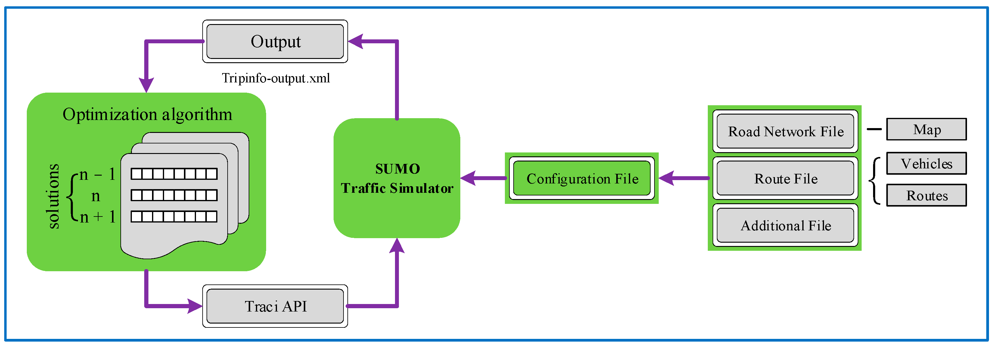
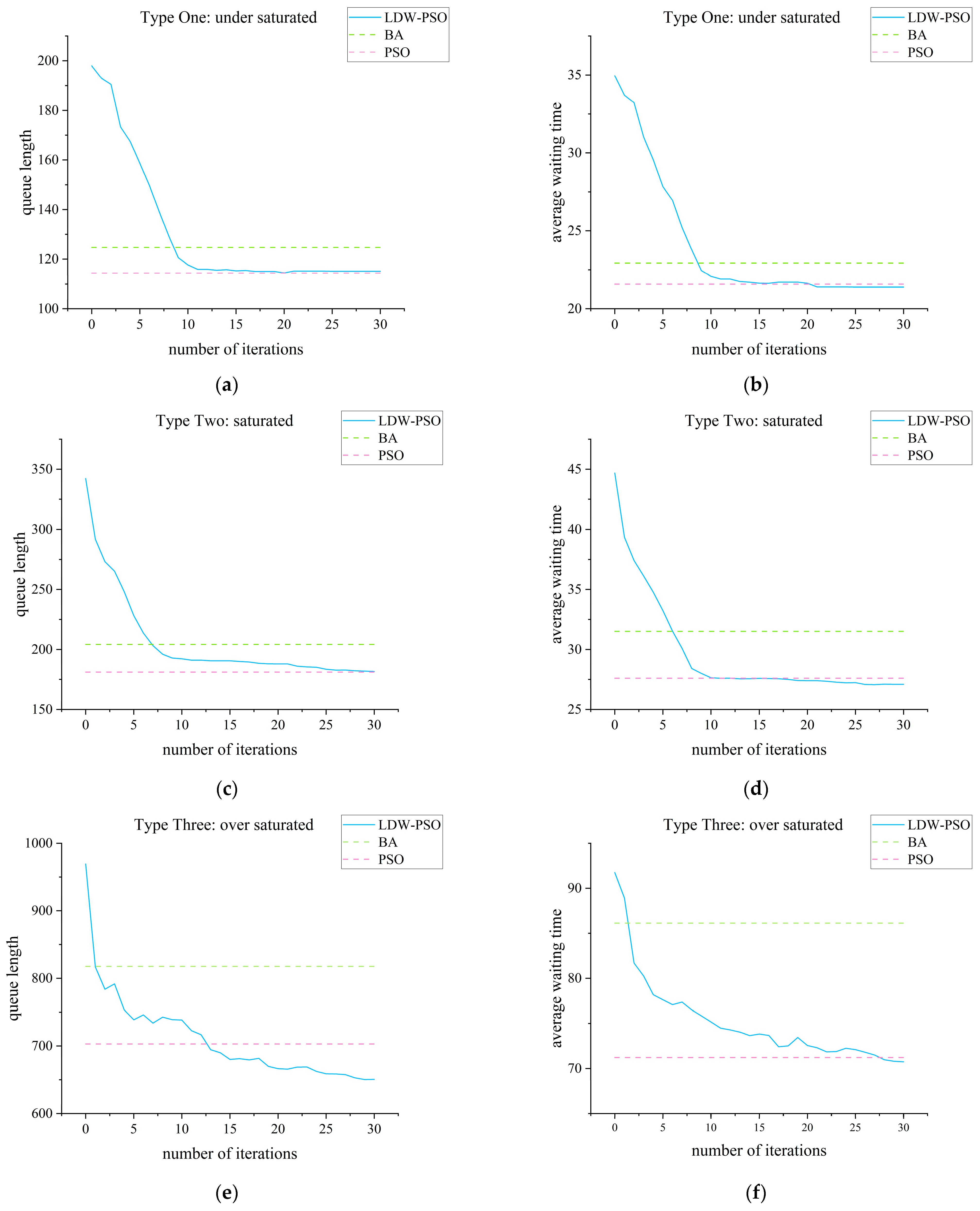
- Combing SUMO and LDW-PSO, a new model is proposed to reduce queue length and average waiting time in an isolated intersection with hundreds of vehicles. Besides, the objective function’s property is evaluated by this paper.
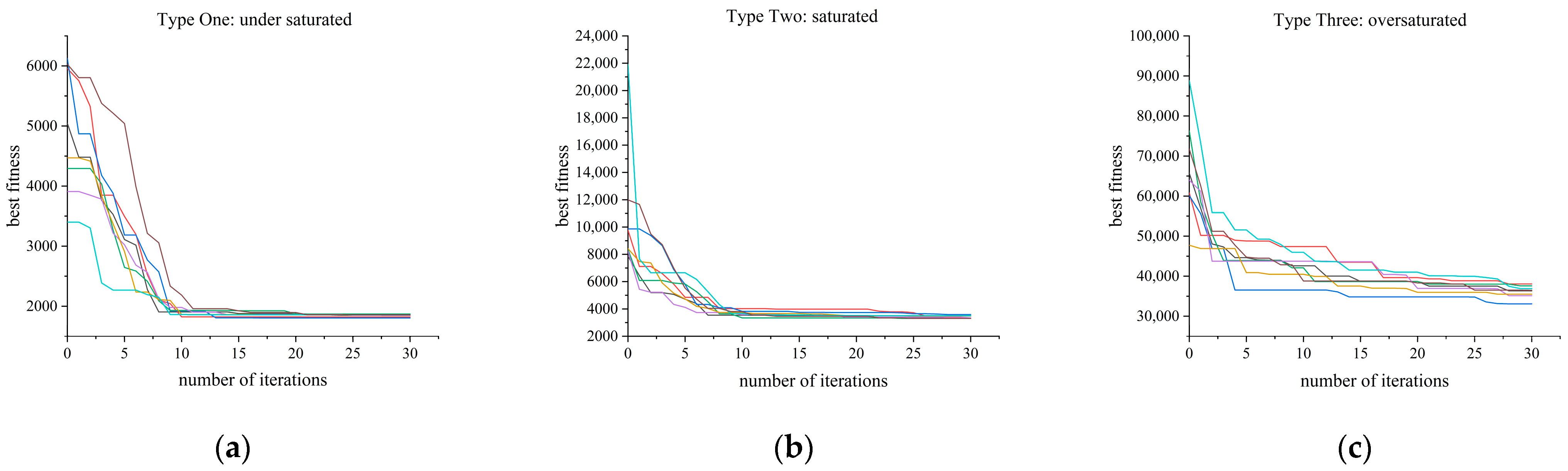
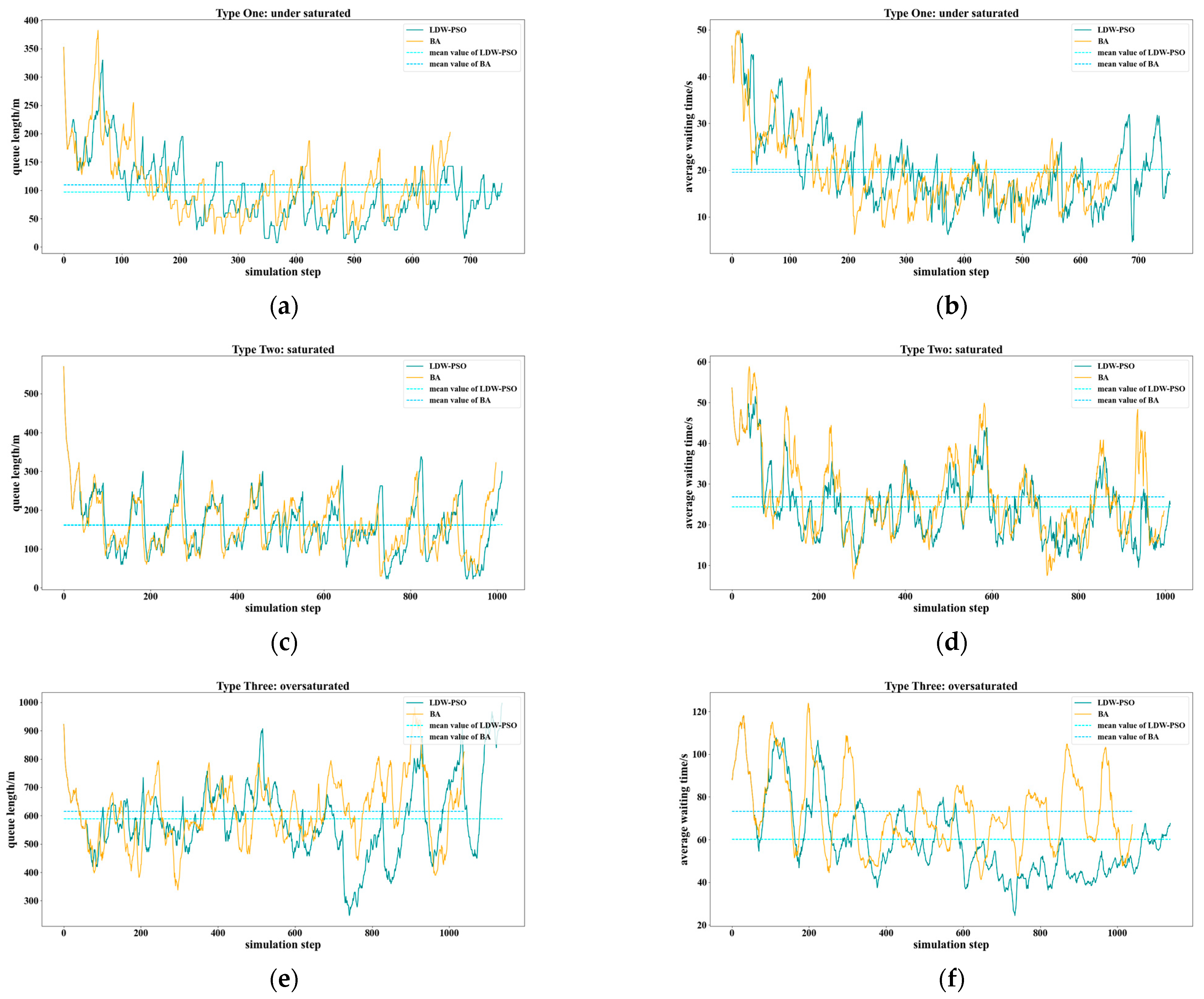
- Our experiment with traffic data is analysed under three conditions: under saturated, saturated, and oversaturated, compared with previous works only considering one specific scenario. Besides, more than 900 vehicles are simulated in oversaturated conditions to represent the high load state, which is a big challenge.
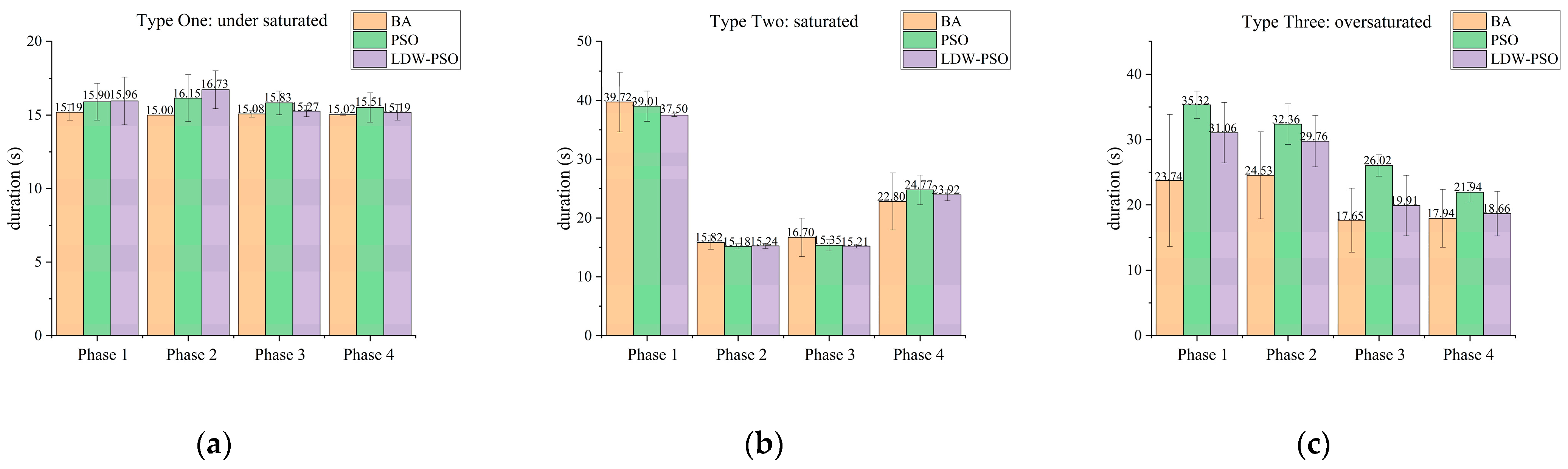
- Further comparisons against B.A., standard PSO optimisation method justify the property of the LDW-PSO. In this paper, the results obtained by LDW-PSO are compared with B.A., which is rarely compared by previous studies.
2. Related Work
3. Background
3.1. Simulaiton of Urban Mobility
3.2. Optimization Algorithms
| Algorithm 1. B.A.—Bat Algorithm. | |
| 1. | |
| 2. | |
| 3. | |
| 4. | |
| 5. | |
| 6. | |
| 7. | |
| 8. | |
| 9. | |
| 10. | |
| 11. | |
| 12. | end if |
| 13. | |
| 14. | |
| 15. | if (bfnew < bf&uniform(0,1) < A) do |
| 16. | |
| 17. | |
| 18. | end if |
| 19. | end while |
| 20. | |
| 21. | end while |
- is the local best solution of particle
- is the global best solution of all particles
- and refer to the position of particle in iteration and
- and represents the velocity of particle in iteration and
- is the initial weight
- is the maximum weight
- refers to the total iterations
- refers to the current iteration
| Algorithm 2. LDW-PSO—Particle Swarm Optimization with Linearly Decreasing Weight. | |
| 1. | |
| 2. | |
| 3. | |
| 4. | |
| 5. | |
| 6. | |
| 7. | |
| 8. | |
| 9. | |
| 10. | |
| 11. | |
| 12. | |
| 13. | |
| 14. | |
| 15. | end if |
| 16. | end while |
| 17. | |
| 18. | end while |
4. Objective Function of the Simulation Model
- refers to the index of all phases in a traffic cycle.
- represents the duration of the green time on phase .
- is the index of discretised green time duration of phase .
- represents all vehicular routes that allow vehicles to pass in phase .
- is the vehicle number of halting vehicles on route on time of phase , and a halting vehicle is defined as its speed below 0.1 m/s.
- refers to the waiting time of vehicle on time of phase . Specifically, the vehicle’s waiting time is accumulated over a specific time interval, rather than the time spent with a speed below 0.1 m/s since the last time it was faster than 0.1 m/s.
- is the previously defined traffic load from road heading to road .
- is the total number of vehicles from heading to road , including halting vehicles and moving vehicles.
- represents the number of vehicles that can cross the intersection through the remaining time of phase .
- refers to the remaining capacity of road that can be changed over time but limited by the maximum capacity of the outgoing road as defined in (13).
5. Simulation and Results
5.1. Design of Experiment on SUMO
5.2. Results and Discussions
6. Conclusions and Future Works
Author Contributions
Funding
Institutional Review Board Statement
Informed Consent Statement
Data Availability Statement
Conflicts of Interest
Glossary
| Optimisation Algorithm: Bat Algorithm | |
| i | Each bat in the bat population |
| xi | Position of bat i |
| vi | Velocity of bat i |
| xbest | Global optimal solution of the bat algorithm |
| t | Current generation |
| Q | Frequency |
| LBb | Lower boundary of position |
| UBb | Upper boundary of position |
| A | Loudness |
| r | Pulse |
| bf | Fitness of bat |
| Optimisation Algorithm: Particle Swarm Optimization with Linearly Decreasing Weight | |
| j | Each particle in the particle swarm |
| xj | Position of particle j |
| vj | Velocity of particle j |
| pbest | Local best solution of each generation |
| gbest | Global best solution of the LDW-PSO |
| c1 | Self-learning factor |
| c2 | Global learning factor |
| ω | Inertia weight of particle |
| Ngen | Max generation |
| g | Current generation |
| Npop | Max population |
| LBP | Lower boundary of position |
| UBP | Upper boundary of position |
| LBv | Lower boundary of velocity |
| UBv | Upper boundary of velocity |
| pf | Fitness of particle |
| Objective Function of The Simulation Model | |
| n | Index of all phases in a traffic cycle |
| GTn | Duration of the green time on phase n |
| d | Index of discretised green time duration of phase n |
| S | Summation of three parts |
| Tw | Waiting time |
| Tq | Loss of start-stop time |
| Tp | Time reward |
| LB | Lower boundary of effective green time of each phase |
| UB | Upper boundary of effective green time of each phase |
| (v,w) | Vehicular route from road v heading to road w |
| L | Traffic load |
| R | All vehicular routes that allow vehicles to pass |
| VN | Vehicle number of halting vehicles |
| WT | Waiting time |
| θT | Linear function represents the start-stop delay |
| MC | Maximum capacity |
| PV | Number of vehicles that can pass through the intersection |
| TN | Total number o vehicles, including halting and moving vehicles |
| RT | Number of vehicles that can cross the intersection through the remaining time |
| RC | Remaining capacity |
References
- United Nations. World Urbanization Prospects: The 2018 Revision; Economic & Social Affairs: New York, NY, USA, 2018; pp. 1–2. [Google Scholar]
- McCrea, J.; Moutari, S. A hybrid macroscopic-based model for traffic flow in road networks. Eur. J. Oper. Res. 2010, 207, 676–684. [Google Scholar] [CrossRef]
- Ye, B.L.; Wu, W.M.; Gao, H.M.; Lu, Y.X.; Cao, Q.Q.; Zhu, L.J. Stochastic Model Predictive Control for Urban Traffic Networks. Appl. Sci. 2017, 7, 588. [Google Scholar] [CrossRef] [Green Version]
- Hu, W.; Wang, H.; Yan, L.; Du, B. A swarm intelligent method for traffic light scheduling: Application to real urban traffic networks. Appl. Intell. 2016, 44, 208–231. [Google Scholar] [CrossRef]
- de Oliveira, L.F.P.; Manera, L.T.; da Luz, P.D.G. Development of a Smart Traffic Light Control System with Real-Time Monitoring. IEEE Internet Things J. 2021, 8, 3384–3393. [Google Scholar] [CrossRef]
- Hu, W.B.; Wang, H.; Min, Z.Y. A storage allocation algorithm for outbound containers based on the outer-inner cellular automaton. Inf. Sci. 2014, 281, 147–171. [Google Scholar] [CrossRef]
- Gartner, N.H.; Pooran, F.J.; Andrews, C.M. Optimised policies for adaptive control strategy in real-time traffic adaptive control systems—Implementation and field testing. Transp. Res. Rec. J. Transp. Res. Board 2002, 1811, 148–156. [Google Scholar] [CrossRef]
- Zhou, P.; Fang, Z.; Dong, H.; Liu, J.; Pan, S. Data Analysis with Multi-objective Optimisation Algorithm: A Study in Smart Traffic Signal System. In Proceedings of the 2017 IEEE/Acis 15th International Conference on Software Engineering Research, Management and Applications, London, UK, 7–9 June 2017; pp. 307–310. [Google Scholar]
- Karakuzu, C.; Demirci, O. Fuzzy logic based smart traffic light simulator design and hardware implementation. Appl. Soft. Comput. 2010, 10, 66–73. [Google Scholar] [CrossRef]
- Sanchez, J.; Galan, M.; Rubio, E. Applying a traffic lights evolutionary optimisation technique to a real case: “Las Ramblas” area in Santa Cruz de Tenerife. IEEE Trans. Evol. Comput. 2008, 12, 25–40. [Google Scholar] [CrossRef]
- Chou, L.D.; Shen, T.Y.; Tseng, C.W.; Chang, Y.J.; Kuo, Y.W. Green wave-based virtual traffic light management scheme with VANETs. Int. J. Ad Hoc Ubiquitous Comput. 2017, 24, 22–32. [Google Scholar] [CrossRef]
- Phuong Thi Mai, N.; Passow, B.N.; Yang, Y. Improving Anytime Behavior for Traffic Signal Control Optimization Based on NSGA-II and Local Search. In Proceedings of the 2016 International Joint Conference on Neural Networks, Vancouver, BC, Canada, 24–29 July 2016; pp. 4611–4618. [Google Scholar]
- Ardiyanto, I.; Sulistyo, S. A Study on Metaheuristics for Urban Traffic Light Scheduling Problems. In Proceedings of the 2018 the 10th International Conference on Information Technology and Electrical Engineering, Bali, Indonesia, 24–26 July 2018; pp. 545–550. [Google Scholar]
- Garcia-Nieto, J.; Alba, E.; Olivera, A.C. Swarm intelligence for traffic light scheduling: Application to real urban areas. Eng. Appl. Artif. Intell. 2012, 25, 274–283. [Google Scholar] [CrossRef]
- Olivera, A.C.; Garcia-Nieto, J.M.; Alba, E. Reducing vehicle emissions and fuel consumption in the city by using particle swarm optimisation. Appl. Intell. 2015, 42, 389–405. [Google Scholar] [CrossRef]
- Shi, Y.; Liu, H.C.; Gao, L.; Zhang, G.H. Cellular particle swarm optimisation. Inf. Sci. 2011, 181, 4460–4493. [Google Scholar] [CrossRef]
- Montes de Oca, M.A.; Stutzle, T.; Birattari, M.; Dorigo, M. Frankenstein’s PSO: A Composite Particle Swarm Optimization Algorithm. IEEE Trans. Evol. Comput. 2009, 13, 1120–1132. [Google Scholar] [CrossRef]
- Srivastava, S.; Sahana, S.K. Bat Algorithm-Based Traffic Signal Optimization Problem. In Soft Computing for Problem Solving, Socpros 2017; Springer: Singapore, 2019; Volume 1, pp. 927–936. [Google Scholar]
- He, J.J.; Hou, Z.E. Ant colony algorithm for traffic signal timing optimisation. Adv. Eng. Softw. 2012, 43, 14–18. [Google Scholar] [CrossRef]
- Celtek, S.A.; Durdu, A.; Ali, M.E.M. Real-time traffic signal control with swarm optimisation methods. Measurement 2020, 166, 7. [Google Scholar] [CrossRef]
- Galvan-Correa, R.; Olguin-Carbajal, M.; Herrera-Lozada, J.C.; Sandoval-Gutierrez, J.; Serrano-Talamantes, J.F.; Cadena-Martinez, R.; Aquino-Ruiz, C. Micro Artificial Immune System for Traffic Light Control. Appl. Sci. 2020, 10, 7933. [Google Scholar] [CrossRef]
- Peres, M.; Ruiz, G.; Nesmachnow, S.; Olivera, A.C. Multi-objective evolutionary optimisation of traffic flow and pollution in Montevideo, Uruguay. Appl. Soft. Comput. 2018, 70, 472–485. [Google Scholar] [CrossRef]
- Damay, N. Multiple-Objective Optimisation of Traffic Lights Using a Genetic Algorithm and a Microscopic Traffic Simulator. 2015. Available online: http://www.diva-portal.org/smash/get/diva2:816306/FULLTEXT01.pdf (accessed on 10 November 2021).
- Jintamuttha, K.; Watanapa, B.; Charoenkitkarn, N. Dynamic Traffic Light Timing Optimization Model Using Bat Algorithm. In Proceedings of the 2016 2nd International Conference on Control Science and Systems Engineering, Singapore, 27–29 July 2016; pp. 181–185. [Google Scholar]
- Yang, X.S. A New Metaheuristic Bat-Inspired Algorithm. In Nature Inspired Cooperative Strategies for Optimization; Springer: Berlin, Germany, 2010; pp. 65–74. [Google Scholar]
- Eberhart, R.; Kennedy, J. A new optimiser using particle swarm theory. In Proceedings of the Sixth International Symposium on Micro Machine and Human Science (Cat. No. 95TH8079) MHS’95, Nagoya, Japan, 4–6 October 1995; pp. 39–43. [Google Scholar] [CrossRef]


| Settings | North | South | West | East |
|---|---|---|---|---|
| Road length (m) | 2280 | 1650 | 1620 | 727.5 |
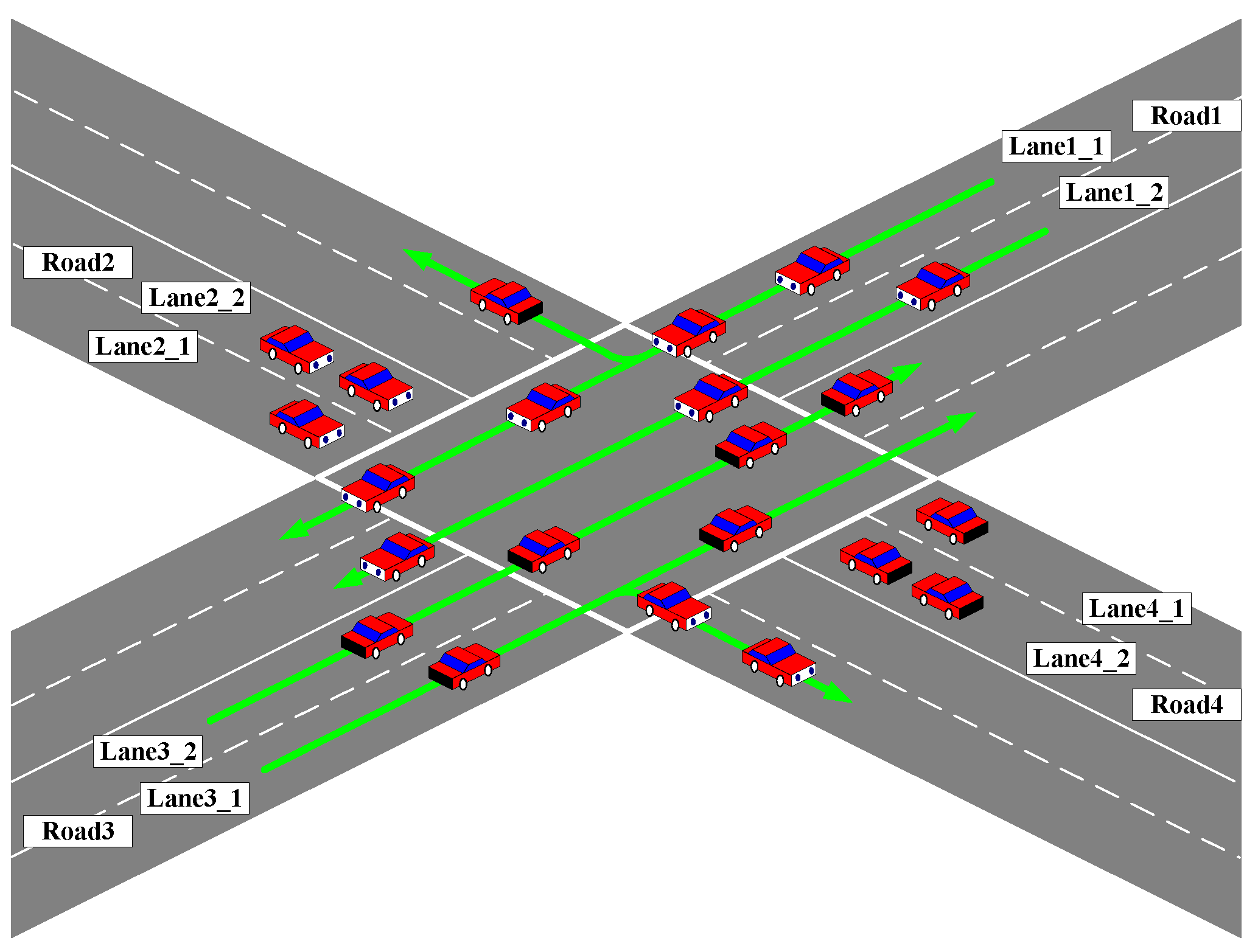
| Number of lanes | 2 | 2 | 4 | 4 |
| Maximum capacity | 608 | 440 | 864 | 324 |
| Outgoing Direction | From North | From South | From West | From East |
|---|---|---|---|---|
| Right (%) | 40.0 | 40.0 | 15.0 | 15.0 |
| Straight (%) | 20.0 | 20.0 | 70.0 | 70.0 |
| Left (%) | 40.0 | 40.0 | 15.0 | 15.0 |
| Type | Arrival Rate (Vehicles/min) | East (%) | West (%) | North (%) | South (%) |
|---|---|---|---|---|---|
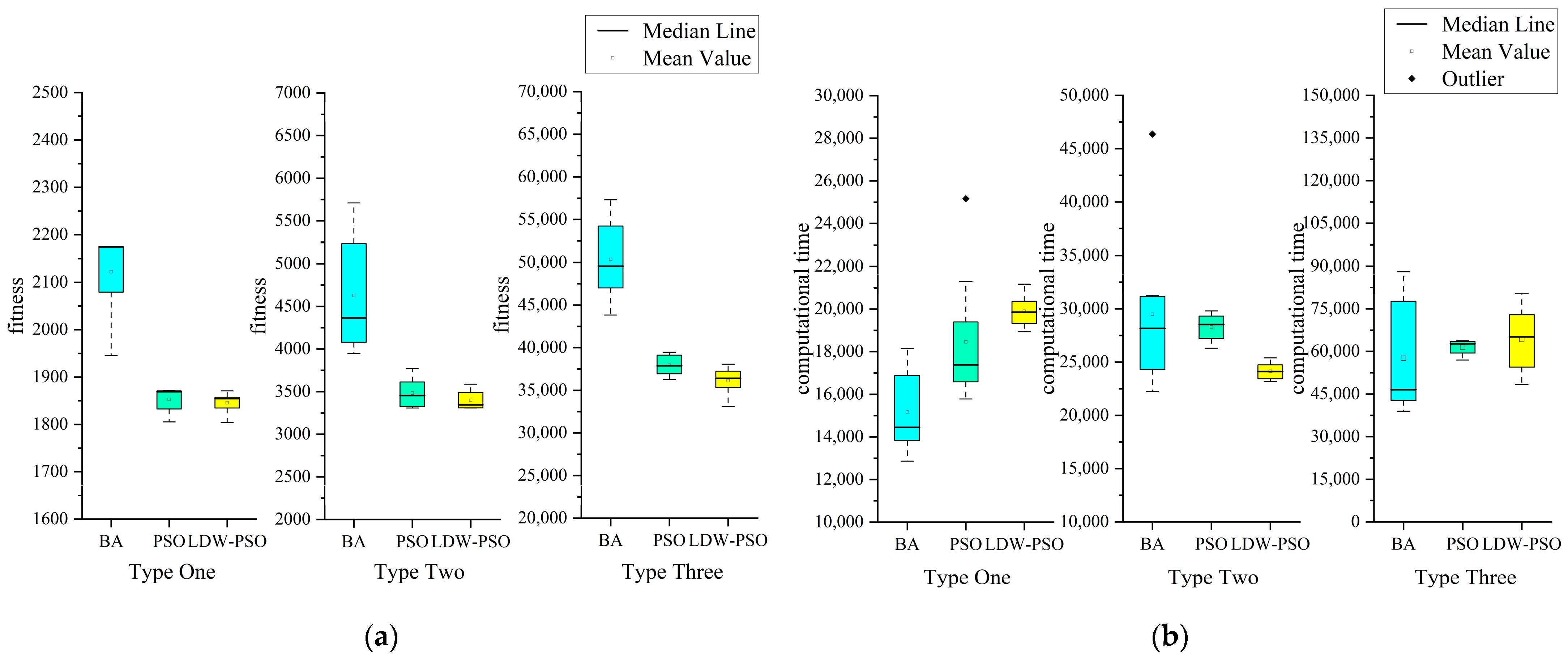
| Type One: under saturated | 45 | 18.60 | 33.73 | 25.18 | 22.49 |
| Type Two: saturated | 60 | 26.71 | 51.24 | 12.00 | 10.05 |
| Type Three: oversaturated | 75 | 20.60 | 45.71 | 19.57 | 14.12 |
| Types | Settings | Value |
|---|---|---|
| Simulation | Maximum simulation time (s) | 2400 |
| Number of cycles | 10 | |
| Maximum number of evaluations per simulation | 600 | |
| Vehicle | Average vehicle length (m) | 5.0 |
| Average vehicle gap (m) | 2.5 | |
| ) | 1.5 | |
| ) | 4.5 | |
| ) | 120 | |
| BA | Number of generations | 30 |
| Size of population | 20 | |
| Loudness | 0.7 | |
| Pulse | 0.5 | |
| Frequency range | [0, 6] | |
| Position range | [15, 50] | |
| Standard PSO | Number of generations | 30 |
| Size of population | 20 | |
| 1.49445 | ||
| 0.729 | ||
| Position range | [15, 50] | |
| Velocity range | [−4, 4] | |
| LDW-PSO | Number of generations | 30 |
| Size of population | 20 | |
| 2/2 | ||
| 0.9/0.4 | ||
| Position range | [15, 50] | |
| Velocity range | [−4, 4] |
Publisher’s Note: MDPI stays neutral with regard to jurisdictional claims in published maps and institutional affiliations. |
© 2021 by the authors. Licensee MDPI, Basel, Switzerland. This article is an open access article distributed under the terms and conditions of the Creative Commons Attribution (CC BY) license (https://creativecommons.org/licenses/by/4.0/).
Share and Cite
Shi, Y.; Qi, Y.; Lv, L.; Liang, D. A Particle Swarm Optimisation with Linearly Decreasing Weight for Real-Time Traffic Signal Control. Machines 2021, 9, 280. https://doi.org/10.3390/machines9110280
Shi Y, Qi Y, Lv L, Liang D. A Particle Swarm Optimisation with Linearly Decreasing Weight for Real-Time Traffic Signal Control. Machines. 2021; 9(11):280. https://doi.org/10.3390/machines9110280
Chicago/Turabian StyleShi, Yanjun, Yuhan Qi, Lingling Lv, and Donglin Liang. 2021. "A Particle Swarm Optimisation with Linearly Decreasing Weight for Real-Time Traffic Signal Control" Machines 9, no. 11: 280. https://doi.org/10.3390/machines9110280
APA StyleShi, Y., Qi, Y., Lv, L., & Liang, D. (2021). A Particle Swarm Optimisation with Linearly Decreasing Weight for Real-Time Traffic Signal Control. Machines, 9(11), 280. https://doi.org/10.3390/machines9110280