The Deterministic Nature of Sensor-Based Information for Condition Monitoring of the Cutting Process

Abstract

Condition monitoring of the cutting process is a core function of autonomous machining and its success strongly relies on sensed data. Despite the enormous amount of research conducted so far into condition monitoring of the cutting process, there are still limitations given the complexity underlining tool wear; hence, a clearer understanding of sensed data and its dynamical behavior is fundamental to sustain the development of more robust condition monitoring systems. The dependence of these systems on acquired data is critical and determines the success of such systems. In this study, data is acquired from an experimental setup using some of the commonly used sensors for condition monitoring, reproducing realistic cutting operations, and then analyzed upon their deterministic nature using different techniques, such as the Lyapunov exponent, mutual information, attractor dimension, and recurrence plots. The overall results demonstrate the existence of low dimensional chaos in both new and worn tools, defining a deterministic nature of cutting dynamics and, hence, broadening the available approaches to tool wear monitoring based on the theory of chaos. In addition, recurrence plots depict a clear relationship to tool condition and may be quantified considering a two-dimensional structural measure, such as the semivariance. This exploratory study unveils the potential of non-linear dynamics indicators in validating information strength potentiating other uses and applications.

1. Introduction

Since the late 1990s, we have witnessed a change from the old practice of changing tools automatically to the feasibility of instituting tool change procedures based on monitoring the amount of wear on the cutting tool-edges through the implementation of adaptive tool inspection mechanisms [1,2]. Literature reports numerous proposals for the architecture of condition monitoring systems for online supervision and control. Nevertheless, few of the architectures have gained sufficient acceptance or otherwise proved to be feasible for most machining processes/conditions. One important strategy to support this goal is sensor-based and real-time control of key characteristics of both machines and products, throughout the manufacturing process [3,4,5]. The development of such systems considers the traditional ability of the operator to determine the condition of the tool based on his/her experience and senses, e.g., vision and hearing. Sensor-based information and its deterministic nature is, hence, of vital importance towards the development of reliable condition monitoring systems.

The literature reports numerous examples pertaining to the study of sensor feasibility regarding tool condition monitoring [6,7,8,9,10], and, from this research, a large variety of sensors/attributes have been proposed. Previous work on the relationship between audible emissions and tool wear has established that audible emissions are capable of indicating the extent of the cutting edge wear, as in Weller et al. [11]. McNulty et al. [12] have also highlighted the use of noise spectra for tool life evaluation applied to several cutting processes and have found significant changes in power in certain frequency bands that appear to be characteristic of wear in certain cutting processes. Lee [13] found that, during turning, the machine noise exhibited a wear-related change of sound pressure level (SPL) at certain frequencies (4–6 kHz) for several materials. A drop in the SPL before the tertiary zone (third and last stage of wear) was suggested as an end of tool-life predictor. Experiments carried out by Ya et al. [14], using two different types of turning tools, showed that both the tool angle and the cutting speed exerted no great influence on the average cutting noise. Vibration has also been used to recognize the wear state of a tool whilst turning [15], and the main advantage of this method is that it is easily applied. Wear monitoring of cutting tools has been performed using many different sensing techniques, including; temperature, motor current, acoustic emission (AE), audible emissions, vibration, and force [7,9,16,17], to name a few. Some of these have been successfully applied under laboratory conditions, but their success was limited in industrial applications. An understanding of the underlying mechanisms and models are essential for an effective fault and monitoring system’s development [18].

Despite the enormous amount of work developed so far, it is recognized that forecasting in complex systems that are poorly understood, noisy, and often non-linear can be practically impossible when based on traditional model predictive algorithms, Parlos et al. [19] and Li [20]. The complexity inherent to these systems led scientists to model processes through system identification techniques. Clearly, the quality of sensor information leads to promising results concerning the detection of the state of wear in idealized conditions but much research has to be conducted in information processing, modeling and decision making in order to correctly classify the tool wear state from the available sensors under different cutting conditions [21,22,23,24]. The common factor in all these research projects is the attempt to develop an effective and efficient Tool Condition Monitoring that supports unmanned machining. A reliable system should integrate different information sources and must be based on reliable sources so that a robust system can be built [8]. Although multisensory integration has proven to improve the performance, it does most often rely on the stationary assumption of acquired signals and, hence, disregard fractal or self-similar characteristics of sensed data [25]. In this sense, capturing the non-linear or non-stationary properties of sensed data provides important added information to support more reliable condition monitoring systems.

Machining causes an interaction between the tool and the workpiece that leads to vibrations during the cutting process. Large amplitude vibrations are known as chatter and result in poor finishing and tool life shortening [22]. The non-linearities that characterize noisy information and non-linear dynamics are inherent to condition monitoring and call for a better understanding of sensed information [26]. Being non-linear, a system can be described by non-linear equations, but these are difficult to solve and often are approximated by linear equivalents that help attaining a solution, often disregarding the chaotic behavior underneath. Given the noisy characteristic of sensor-based information and the challenging task of modeling the cutting process, most often, tool wear monitoring is performed using artificial intelligence techniques, such as neural networks [27,28], taking advantage of their ability to model even the most complex non-linear functions. Nevertheless, artificial neural networks, or other modeling techniques, take into account pre-selected features or attributes to characterize the process being modeled, often collected from sensed information that is sensitive to the number of data points in the sample, sampling frequency, and signal-to-noise ratio [8]. In addition, if, in fact, those sensors capture the inherent dynamics, it is often necessary to determine whether the collected information carries enough information for the purpose of condition monitoring or, otherwise, has no contribution at all.

Although a newcomer, chaos theory has proven to find a place in different fields of research, such as energy [29], health [30,31], computing [32], and hydrology [33], and many others, such as meteorology, economy, biomedicine, sociology, bioinformatics, chemistry, or astrophysics [21]. Chaos is a term used to characterize apparently disordered deterministic non-linear systems with random-like behavior that are sensitive to initial conditions [34,35]. Deterministic systems may become unpredictable in the long term, and such evolution is the subject for chaos theory [36]. This behavior is evident in the cutting process, as shown by Grabec [37,38], being characterized by a complex and random-like behavior [26,39]. There were attempts to model this non-linear behavior relating the forces originated during cutting with the depth of cut, but these tended to be unstable and subject to limited boundaries upon cutting conditions. Chatter is a common manifestation of the random-like behavior that characterizes hard cutting and is normally avoided through manipulation of cutting conditions [40,41,42]. Further, there are also cumulative origins for the random-like behavior associated with the fact that cutting tools, as well as work pieces, are not uniform. The given behavior cannot be associated to machine noise since it pertains to frequencies well above any machine borne noise [42]. The presented study takes into consideration the underlying mechanisms of sensed signals as being deterministic and chaotic, as demonstrated by several authors, such as Moon and Abarbanel [42] and Grabec [37,38]. The strong dependency of condition monitoring systems on sensed information demands a better understanding of sensed signals and their deterministic nature and, hence, determining the feasibility of such systems to forecast under such complex behavior. Considering the limited literature available on chatter, tool wear and non-linear behavior during cutting, it is possible to depict a great impact these may have on tool life and wear.

A clear understanding of the sensed data and its dynamical behavior is fundamental for a proper extraction, use, and understanding of condition monitoring indicators and, hence, sensed information should be further explored to legitimate poorly understood relationships to cutting tool wear. This paper explores the deterministic nature of sensed information using different techniques, such as the Lyapunov exponent, mutual information, attractor dimension, and recurrence plots.

2. Theoretical Background on Non-Linear Indicators

There are two fundamental approaches when it comes to identifying chaos that consist of graphical/qualitative or quantitative methods. Graphical methods are visually more attractive and allow for deeper interpretations, although they sometimes lack the essential deterministic inference [34,43]. There are some well-studied techniques allowing visualization, such as phase space plots, power spectrum maps, and recurrent maps [36,44]. Nevertheless, graphical methods are not subject to objective conclusions and might give rise to different interpretations and, fundamentally, are not quantifiable and, hence, not prone to be integrated in unmanned automation. There are a few quantifiers that support a more objective measure of chaos or random-like behaviors, and these are: entropy, Lyapunov exponent, fractal dimension, and correlation dimension [36,38,45,46]. These indicators are fundamental for an unbiased discussion regarding the importance of sensed data and their role in the development of condition monitoring systems being industrial, medical, or otherwise general systems using sensed data. It should be emphasized that the growing numbers of autonomous systems rely on sensed information in order to interact with the environment, e.g., robotics.

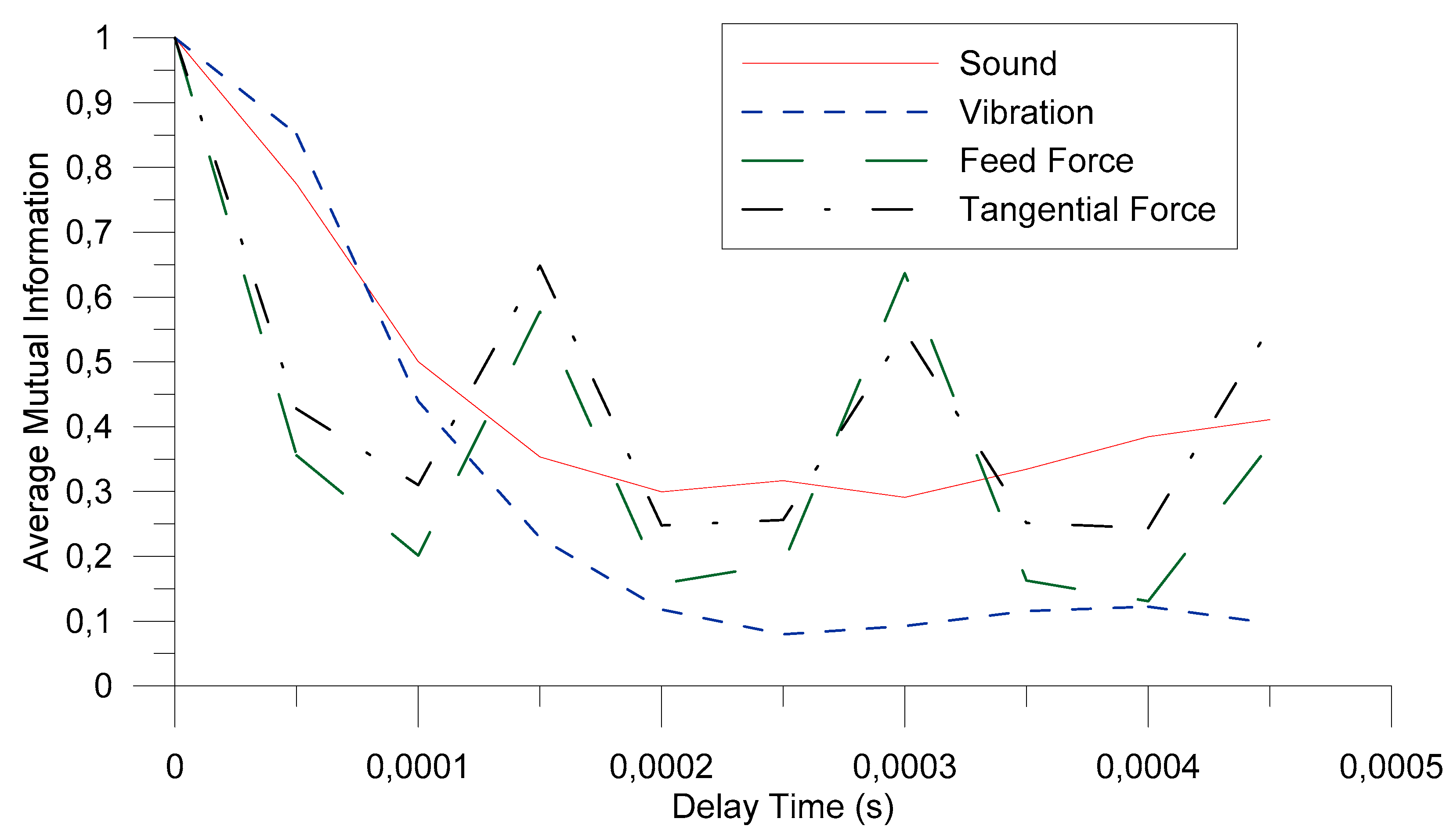
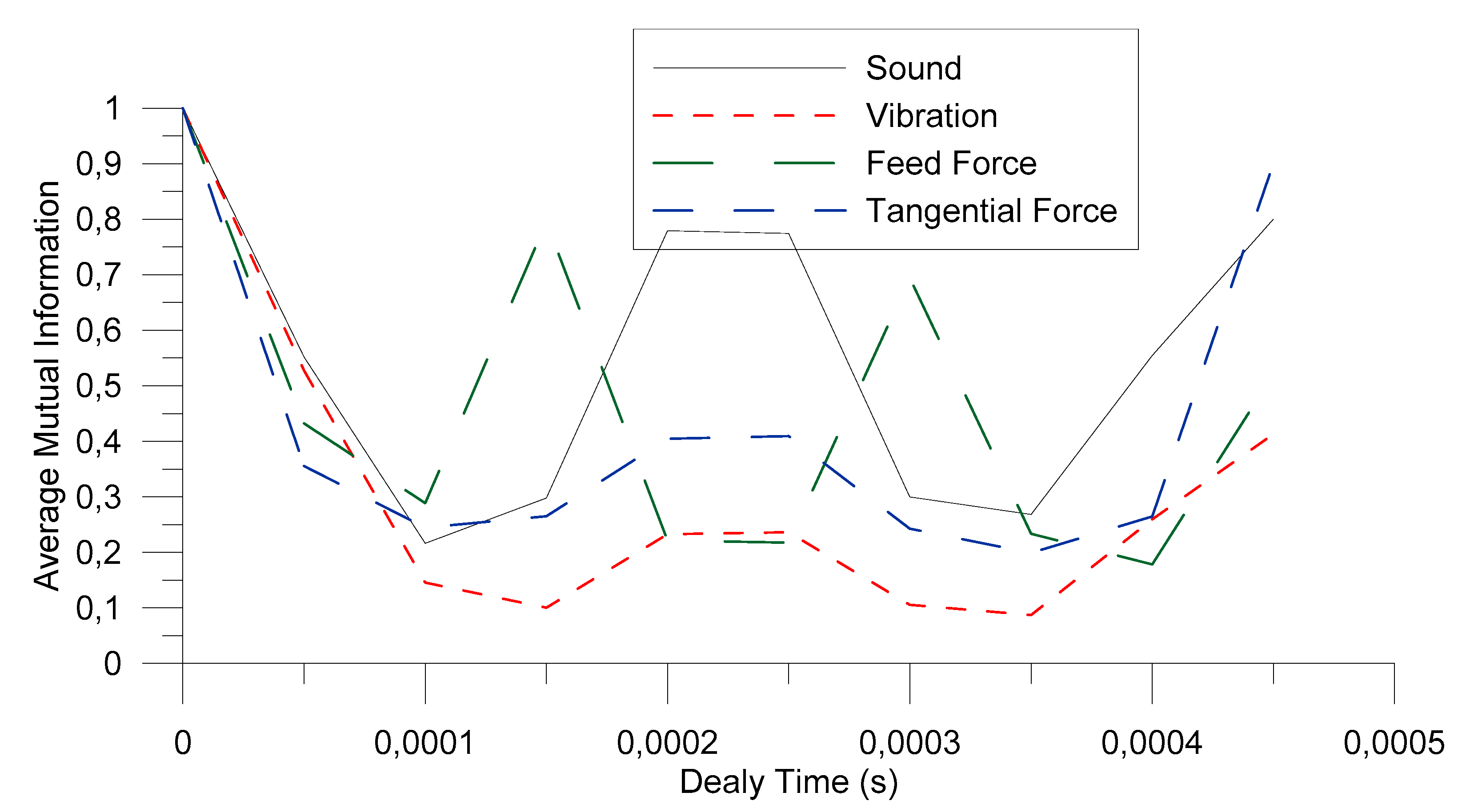
2.1. Average Mutual Information

Given the complexity of the underlying system dynamics, one relies on time-series to perform an evaluation of the deterministic behavior of the cutting process. Tool condition monitoring implies data collection from different sources that assume a temporal sequence format, providing the basis for diagnosing, i.e., x_i, where i represents the sample sequence number that finds correspondence in a time scale according to the sampling period. Taken’s theorem (Takens [47]) states that the dynamics of a time series are fully captured in an m dimensional phase space which is as least the dimension of the original attractor. The reconstructed phase space can be built from the time series using the delay method introduced by Fraser and Swinney [48], as follows:

$$y_i=[x_i,x_{i-\tau },x_{i-2\tau },\dots ,x_{i-(m-1)\tau }],$$

(1)

where τ is the time delay and m the embedding dimension. Determining appropriate parameters is not trivial and might be done using the Average Mutual Information (AMI) (Fraser and Swinney [48]), Autocorrelation Function (ACF) [49], or Correlation Integral (CI) [50]. From these methods, the Average Mutual Information is considered the best since it reflects non-linear properties and, thus, does not require large amounts of data otherwise required by CI and ACF. The AMI approach sets the time delay as the first minimum of the Average Mutual Information, a method suggested by Fraser and Swinney [48]. The AMI is given by

$$I(\tau )=-{\displaystyle \sum _{ij}{p}_{ij}(\tau )\ln \frac{p_{ij}(\tau )}{p_i{p}_j}},$$

(2)

where pi is the probability of finding a time series value in the i-th interval, and p_ij(τ) is the joint probability that an observation falls into the i-th interval and the observation time τ later falls into the j-th interval. The embedding dimension m can be determined using the false nearest neighbor method [51], considering that the attractor of a deterministic system has a smooth and regular shape. It means that, if two points, y_i and y_t, are sufficiently close in the reconstructed attractor, they cannot grow apart more than a given constant.

$$R_i=\frac{\left|x_{i+m\tau }-x_{t+m\tau }\right|}{\Vert y_i-y_t\Vert }.$$

(3)

If R_i is larger than a given threshold, then, y_i is marked as having a false nearest neighbor. Equation (3) must be applied for the whole time series and for various values of m until the fraction of points for which R_i is bigger than the threshold is negligible.

2.2. Lyapunov Exponents

Sensitive dependence on initial conditions can also be performed using Lyapunov exponents and can be used to determine if a given system is chaotic or stable. The so-called Lyapunov exponent captures the rate at which two initially close trajectories on the phase space grow apart [52]. Lyapunov exponents are defined as the average growth rate, λ_i, considering two neighboring points, and, in the ith direction, considering time as t, according to the following formulation [53]:

$${\lambda }_i=\underset{t\to \infty }{{\displaystyle \lim }}\frac{1}{t}{\log }_2\frac{\Vert \delta x_i(t)\Vert }{\Vert \delta x_i(0)\Vert }.$$

(4)

The most important thing to retain is the largest Lyapunov exponent, λ₁, enabling us to depict a chaotic system, hence being sufficient for the present study. The algorithm used to calculate λ₁ is briefly explained and follows the guidelines provided by Wolf et al. [53], which gives a simple implementation method.

$${\lambda }_1=\frac{1}{t_M-t_0}{\displaystyle \sum _{k=1}^M{\log }_2\frac{L\prime (t_k)}{L(t_{k-1})}}.$$

(5)

It is first required to determine the nearest neighbor of initial point y_k. L(t_k) is the Euclidean distance between the initial point and the nearest neighbor. Iterating both points in time for a given time in proportion to the embedding delay τ enables the calculation of the final distance L′(t_k−1).

2.3. Recurrence Plots

Earlier studies using recurrent plots were designed to find non-stationary behavior in dynamic systems [44]. Recurrent plots use a two-dimensional representation where each point represents the distance, in a given graded scale, between two adjacent points in the reconstructed attractor. The absence of a pattern on these plots depicts a system with an underlying random behavior, if, otherwise, there is a depictable structure then the system has a deterministic nature [54]. Recurrence plots, by definition, do not provide a quantitative measure relying on the interpretation of the two-dimensional plot, considering the homogeneity of the structure, where clear patterns depict the stationary nature of the system. Although not in the scope of this paper, a quantitative measure could be obtained from the calculation of its semi-variance and plotted against distance as a variogram [55]. Recurrent plots depicting a homogenous structure demonstrate the stationary nature of signals and, hence, are deterministic, or, otherwise, stochastic.

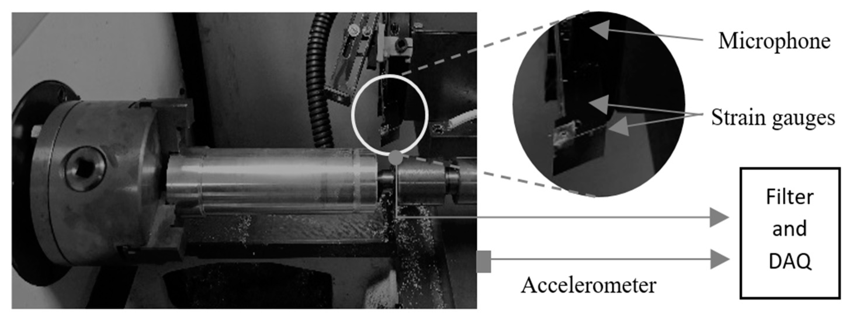
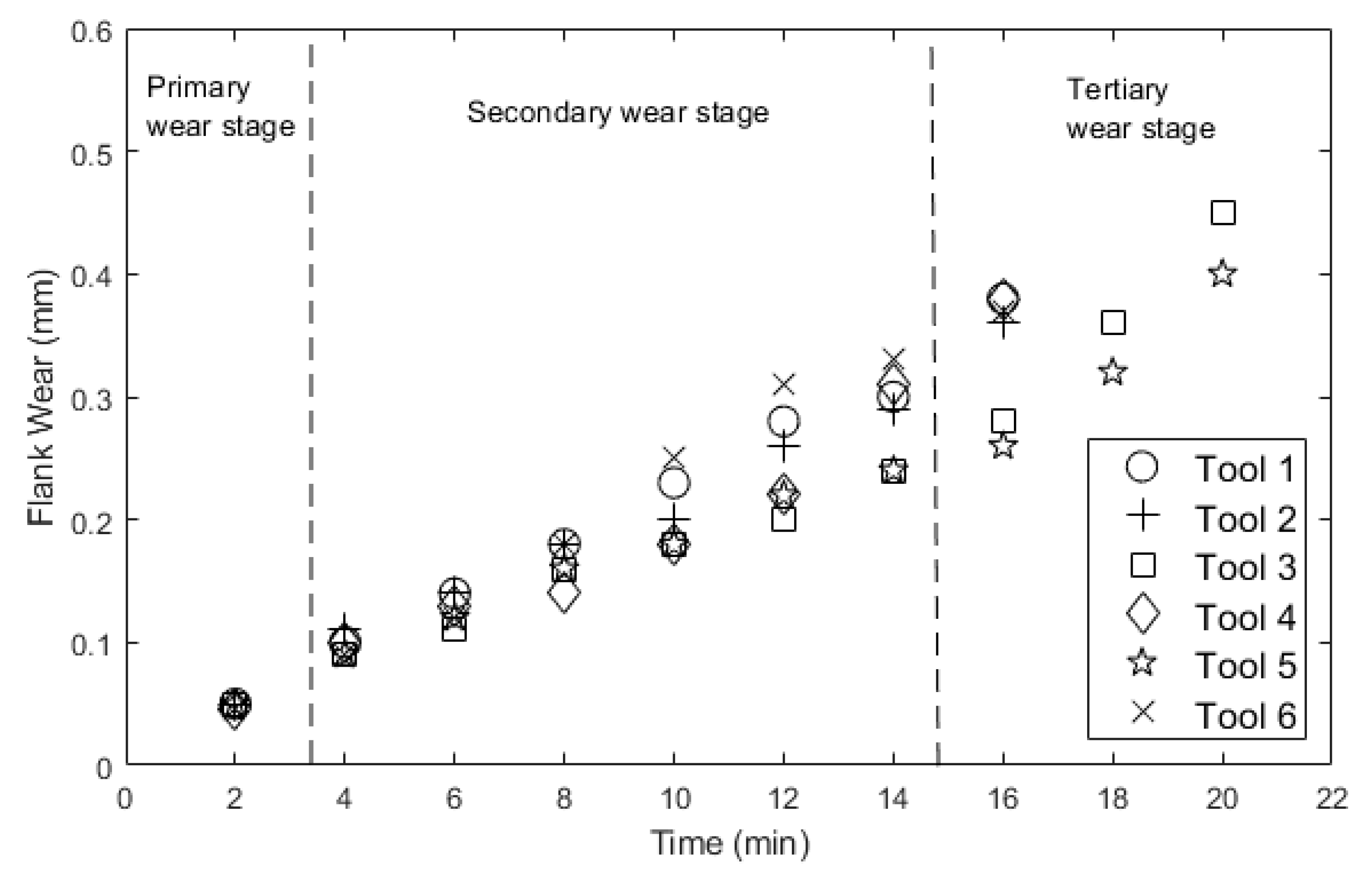
3. Materials and Methods

Considering past research experience [5,8,21,28] and the extensive evidences from literature [1,2,56], background experimental work was conducted on the turning process to collect tool wear data pertaining to sensed vibration, sound, feed, and tangential force. Experimental work was done on a MHP Model Moog-Turn 50 (MT50) Slant Bed Turning Centre (MHP Machines Ltd., Kingsbury, UK), with standard CNC control. The effective bed size is 500 mm with a DC servo motor of 18 kW driving the spindle. This machine can provide a constant power of 34 kW between 1000 and 3000 RPM, and the range of admissible cutting parameters is limited by the maximum 4000 RPM imposed by the chuck capacity. The turning center has the following program resolution: feed rate 0.001 mm/rev; cutting speed 1 m/min; and depth of cut resolution 0.001 mm. Data was acquired from a block of mild steel under realistic production conditions that consisted of a cutting speed of 350 m/min, a feed rate of 0.25 rev/min, and a depth of cut of 1 mm, with an insert type HC-P25 grade (WALTER designation of grade WTN 43) coated carbide (CNMG 120408). The sensors, characteristics and mounting (schematic in Figure 1) can be found in

Table 1. Sensors, characteristics, and mounting.

Scheme	Type	Characteristics	Mounting
Accelerometer	Piezotron Kistler 8752A50	Coupler–Kistler 5108, mounted resonant frequency 32.6 kHz, transverse sensitivity 1.6%, range ±50 g, and sensitivity 100.2 mV/g	Measuring Vertical vibration–Mounted on the base.
Microphone	ECM-1028	Matching amplifier.	10 cm from cutting insert.
Strain gauge	-	Feed and tangential force measurement–two half wheatstone bridge (amplification–RS 435–692) mounting	Tool holder-feed and tangential direction.

.

Data acquisition was performed with a data acquisition board (Amplicon PC30 PGL, Brighton, UK) with a maximum sampling rate of 200 kHz, a typical conversion time of 10 microseconds, and a 16-way multiplexed input, for which Direct Memory Access (DMA) control was used. The analogue signals were sampled at 20 kHz with tool wear and sensor data being acquired at intervals of 2 min, considering an expected tool life, for each insert, of about 15 min. Sample data was recorded for 6 inserts and the length of each sample was 4096 points, and these were acquired approximately in the middle of the bar.

A typical graph of the evolution of flank wear with cutting time, obtained from the experimental work, is shown in Figure 2 and consists of three stages; the first is a short period of rapid wear, and the wear then progresses at a slower rate over a period, in which most of the useful tool life lies. The last stage is a rapid period of accelerated wear, and it is usually recommended that the tool be replaced before this stage. Under the given cutting conditions, the first stage can be observed to end at approximately 3.5 min after the start of cutting, which corresponds to VBB = 0.09 mm, the second stage lies in the interval between 3.5 min and 14.7 min (0.09 < VBB < 0.3 mm), and the third stage starts after 14.7 min of cutting time. The beginning of the third stage coincides with a value of flank wear of 0.3 mm, which is the tool life criterion established in the ISO3685 (1993) standard [57].

The complexity of the cutting dynamics, as well as the noise present in sampled information, makes it difficult to deploy a robust condition monitoring system set to work in real manufacturing conditions. Hence, a deeper understanding on the nature, robustness, and effectiveness of each of the wear-related acquired information is needed. As can be seen from Figure 2, as the tool life comes to its end, there are slight differences in tool life between cutting tips, which proves difficult to anticipate or otherwise model given the wide range of variables governing the cutting process dynamics.

4. Results and Discussion

Based on the earlier description, average mutual information and false nearest neighbors were determined in order to identify the switching dynamics in the time series pertaining to the different sensors. In Figure 3, the average mutual information is plotted against the time lag for each of the sensors, from which the first minimum provides the correct lag time. In the case of new inserts, and from Figure 3, it can be seen that both forces, feed and tangential, present an estimated time delay of 0.1 ms. Sound achieves its first minimum at 0.2 ms, and vibration shows its first minimum at 0.25 ms.

From Figure 4, it can be seen that, for worn inserts, mutual information changes significantly, increased by 25%, having both feed and tangential forces a delay time corresponding to 0.1 ms. Sound has its first minimum at 0.1 ms, and vibration shows its first minimum 0.15 ms. From the difference between time lags for worn and new tools, it can already be seen that the system’s dynamics change as tool wear evolves. The mutual information function of worn tools exhibits an initial stronger gradient than the mutual information function of new tools. This is a strong indication that the system’s dynamics for worn tools are more chaotic (or less predictable) than that for new tools.

To determine the embedding dimension of the underlying system, it is first required to search for the first occurrence of the dimensional state space, where the percentage of false nearest neighbors drops to zero. Figure 5 shows that the number of false nearest neighbors drops to zero for the first time when the embedding dimension reaches 3—the plot for new tools show identical results. This means that the time series signal has an attractor that fully unfolds with an embedding dimension of 3, meaning that the orbits are distinct and do not overlap. In other words, it would be justified to model the behavior of the system with not less than three autonomous first-order ordinary differential equations. The largest Lyapunov exponent was determined according to the approach described and converges to 0.33—this value provides a comprehensive proof that the system demonstrates a chaotic behavior.

The recurrence plot obtained for sound for different tools, in Figure 6 and Figure 7, typifies the encountered behavior underneath the corresponding tools for different tool wear stages. The consistent structures found for the different tools suggest that there is a coherent evolution of the structure that is replicable and should aid in inferencing about its deterministic nature. The transition between recurrence plots from new to almost worn tools illustrates the change in dynamics, depicting the course structure in all worn tools as a more deterministic nature, hence being simpler to model and more predictable in behavior. Completely worn out tools tend to display a fine-grained structure that approximates to the ones produced by random signals, meaning that randomness plays a major role at this stage of wear. It can also be seen that, for worn out tools, recurrent plots are no longer symmetrical on both diagonals, although there is symmetricity along the principle diagonal. One possible candidate explanation might be the occurrence of chatter induced by structural changes promoted by the changes in contact surface between the tool and material being cut. Proving the existence of a chaotic behavior and, hence, the existence of a deterministic behavior would be a pure academic exercise if no further use could be given to these findings. Hence, it is encouraging that the results provided by the recurrence plots offer significant evidence of changes in the systems’ dynamics that are detectable and can be quantifiable, as suggested earlier, considering a two-dimensional structural measure, such as the semivariance.

The importance of these findings stems from the fact that sensed signals, and corresponding sensors, used in condition monitoring are often not assessed from this perspective prior to its utilization, considering that given past evidence regarding the apparent randomness are not conclusive, and the signals may carry tool wear-related information.

5. Conclusions

The renewed interest on the selection criteria of adequate features/sensors for different unmanned systems has placed an increased relevance upon the robustness of information sources. This study explores the deterministic nature of sensed information for condition monitoring providing qualitative and quantitative evidence of their impact. It was found in this study that sensed information from different sensors, widely used for condition monitoring of the cutting process, provide strong evidence that the underlying system exhibits a chaotic behavior, determining that the nature of the cutting process is deterministic. The changes depicted from the recurrent plots at different wear levels suggest its feasibility to detect, or contribute to the detection, of wear level and can be used as a feature on the development of monitoring. As of this stage, there is no measure on the degree of tool wear, although a clear relationship can be depicted. The overall results demonstrate the existence of low dimensional chaos in both new and worn tools, defining a deterministic nature of cutting dynamics and, hence, broadening the available approaches to tool wear monitoring based on the theory of chaos. Findings indicate that recurrence plots can be used to infer upon the degree of tool wear since a consistent and progressive evolution of the two-dimensional mapping can be depicted. Further, this study provides new insights of the underlying dynamics of the cutting process, contributing strongly to an adequate choice of sensors, associated extracted features, and mainly, motivates the exploration of chaos theory applied at an experimental level using real data. This same approach can be used to study the relevance of other information resources being sampled from sensors or otherwise collected from tertiary sources. This study reveals the potential of this technique for tool wear monitoring, but there is still no quantifiable indicator for automated reasoning. Further work should be conducted to quantify the degree to which two-dimensional recurrent maps change according to the corresponding tool wear level, perhaps using a variogram upon the recurrence plot to measure the degree of spatial dependence.

References

1. Ambhore, N.; Kamble, D.; Chinchanikar, S.; Wayal, V. Tool condition monitoring system: A review. Mater. Today Proc. 2015, 2, 3419–3428. [Google Scholar] [CrossRef]
2. Siddhpura, A.; Paurobally, R. A review of flank wear prediction methods for tool condition monitoring in a turning process. Int. J. Adv. Manuf. Technol. 2013, 65, 371–393. [Google Scholar] [CrossRef]
3. Wang, G.F.; Yang, Y.W.; Zhang, Y.C.; Xie, Q.L. Vibration sensor based tool condition monitoring using ν support vector machine and locality preserving projection. Sens. Actuators A Phys. 2014, 209, 24–32. [Google Scholar] [CrossRef]
4. Wang, G.; Guo, Z.; Yang, Y. Force sensor based online tool wear monitoring using distributed Gaussian ARTMAP network. Sens. Actuators A Phys. 2013, 192, 111–118. [Google Scholar] [CrossRef]
5. Silva, R.G.; Wilcox, S.J. Feature evaluation and selection for condition monitoring using a self-organizing map and spatial statistics. Artif. Intell. Eng. Des. Anal. Manuf. 2018, 33, 1–10. [Google Scholar] [CrossRef]
6. Yan, R.; Gao, R.X.; Chen, X. Wavelets for fault diagnosis of rotary machines: A review with applications. Signal Process. 2014, 96, 1–15. [Google Scholar] [CrossRef]
7. Zhu, K.P.; Wong, Y.S.; Hong, G.S. Wavelet analysis of sensor signals for tool condition monitoring: A review and some new results. Int. J. Mach. Tools Manuf. 2009, 49, 537–553. [Google Scholar] [CrossRef]
8. Silva, R.G.; Reuben, R.L.; Baker, K.J.; Wilcox, S.J. Tool wear monitoring of turning operations by neural network and expert system classification of a feature set generated from multiple sensors. Mech. Syst. Signal Process. 1998, 12, 319–332. [Google Scholar] [CrossRef]
9. Snr, D.E.D. Sensor signals for tool-wear monitoring in metal cutting operations—A review of methods. Int. J. Mach. Tools Manuf. 2000, 40, 1073–1098. [Google Scholar]
10. Duro, J.A.; Padget, J.A.; Bowen, C.R.; Kim, H.A.; Nassehi, A. Multi-sensor data fusion framework for CNC machining monitoring. Mech. Syst. Signal Process. 2016, 66–67, 505–520. [Google Scholar] [CrossRef] [Green Version]
11. Weller, E.J.; Scrier, H.M.; Weichbrodt, B. What Sound Can Be Expected from a Worn Tool? ASME Pap. 1969, 91, 525–534. [Google Scholar] [CrossRef]
12. McNulty, G.J.; Popplewell, N. Health Monitoring of Cutting Tools Through Noise Spectra. In Proceedings of the 1st Joint Polytechnic Symposium on Manufacturing Engineering, Leicester, UK, 12–16 July 1997. [Google Scholar]
13. Lee, L.C. A study of noise emission for tool failure prediction. Int. J. Mach. Tool Des. Res. 1986, 26, 205–215. [Google Scholar] [CrossRef]
14. Ya, W.; Shiqiu, K.; Shuzi, Y.; Qilin, Z.; Shanxiang, X.; Yaozu, W. An Experimental Study of Cutting Noise Dynamics. Mach. Dyn. Elem. Vib. 1991, 36, 313–318. [Google Scholar]
15. Dimla, D.; Lister, P. On-line metal cutting tool condition monitoring. Int. J. Mach. Tools Manuf. 2000, 40, 769–781. [Google Scholar] [CrossRef]
16. Huang, P.M.; Lee, C.H. Estimation of tool wear and surface roughness development using deep learning and sensors fusion. Sensors 2021, 21, 5338. [Google Scholar] [CrossRef] [PubMed]
17. Ferrando Chacón, J.L.; de Fernández Barrena, T.; García, A.; de Sáez Buruaga, M.; Badiola, X.; Vicente, J. A Novel Machine Learning-Based Methodology for Tool Wear Prediction Using Acoustic Emission Signals. Sensors 2021, 21, 5984. [Google Scholar] [CrossRef] [PubMed]
18. Orellana, R.; Carvajal, R.; Escárate, P.; Agüero, J.C. On the uncertainty identification for linear dynamic systems using stochastic embedding approach with gaussian mixture models. Sensors 2021, 21, 3837. [Google Scholar] [CrossRef]
19. Parlos, A.G.; Rais, O.T.; Atiya, A.F. Multi-step-ahead prediction using dynamic recurrent neural networks. Neural Netw. 2000, 13, 765–786. [Google Scholar] [CrossRef]
20. Li, X. A brief review: Acoustic emission method for tool wear monitoring during turning. Int. J. Mach. Tools Manuf. 2002, 42, 157–165. [Google Scholar] [CrossRef] [Green Version]
21. Silva, R.G.; Baker, K.J.; Wilcox, S.J.; Reuben, R.L. the Adaptability of a Tool Wear Monitoring System Under Changing Cutting Conditions. Mech. Syst. Signal Process. 2000, 14, 287–298. [Google Scholar] [CrossRef]
22. Rusinek, R.; Wiercigroch, M.; Wahi, P. Modelling of frictional chatter in metal cutting. Int. J. Mech. Sci. 2014, 89, 167–176. [Google Scholar] [CrossRef]
23. Chen, H.Y.; Lee, C.H. Deep learning approach for vibration signals applications. Sensors 2021, 21, 3929. [Google Scholar] [CrossRef]
24. Brili, N.; Ficko, M.; Klančnik, S. Tool condition monitoring of the cutting capability of a turning tool based on thermography. Sensors 2021, 21, 6687. [Google Scholar] [CrossRef]
25. Wang, R.; Song, Q.; Liu, Z.; Ma, H.; Gupta, M.K.; Liu, Z. A novel unsupervised machine learning-based method for chatter detection in the milling of thin-walled parts. Sensors 2021, 21, 5779. [Google Scholar] [CrossRef]
26. Mao, K.; Zhu, M.; Xiao, W.; Li, B. A method of using turning process excitation to determine dynamic cutting coefficients. Int. J. Mach. Tools Manuf. 2014, 87, 49–60. [Google Scholar] [CrossRef]
27. Balazinski, M.; Czogala, E.; Jemielniak, E.; Leski, J. Tool condition monitoring using artificial intelligence methods. Eng. Appl. Artif. Intell. 2002, 15, 73–80. [Google Scholar] [CrossRef]
28. Silva, R.G. Condition monitoring of the cutting process using a self-organizing spiking neural network map. J. Intell. Manuf. 2009, 21, 823–829. [Google Scholar] [CrossRef]
29. Karatasou, S.; Santamouris, M. Detection of low-dimensional chaos in buildings energy consumption time series. Commun. Nonlinear Sci. Numer. Simul. 2010, 15, 1603–1612. [Google Scholar] [CrossRef]
30. Pham, T.D.; Thang, T.C.; Oyama-Higa, M.; Sugiyama, M. Mental-disorder detection using chaos and nonlinear dynamical analysis of photoplethysmographic signals. Chaos Solitons Fractals 2013, 51, 64–74. [Google Scholar] [CrossRef]
31. Keane, C. Chaos in collective health: Fractal dynamics of social learning. J. Theor. Biol. 2016, 409, 47–59. [Google Scholar] [CrossRef] [PubMed]
32. Murillo-Escobar, M.A.; Cruz-Hernández, C.; Abundiz-Pérez, F.; López-Gutiérrez, R.M.; Acosta Del Campo, O.R. A RGB image encryption algorithm based on total plain image characteristics and chaos. Signal Process. 2015, 109, 119–131. [Google Scholar] [CrossRef]
33. Khatibi, R.; Sivakumar, B.; Ali, M.; Kisi, O.; Koçak, K. Investigating chaos in river stage and discharge time series. J. Hydrol. 2012, 414–415, 108–117. [Google Scholar] [CrossRef]
34. Lorenz, E. Deterministic non-periodic flow. J. Atmos. Sci. 1963, 20, 130–141. [Google Scholar] [CrossRef] [Green Version]
35. Devaney, R.L. An Introduction to Chaotic Dynamical Systems; Addison-Wesley Publishing Company, Inc.: Redwood City, CA, USA, 1989. [Google Scholar]
36. Letellier, C. Chaos in nature. In World Scientific Series on Nonlinear Science Series A: Volume 81, 1st ed.; World Scientific: Singapore, 2012; ISBN-10: 9814374423, ISBN-13: 978-9814374422. [Google Scholar]
37. Grabec, I. Chaos generated by the cutting process. Phys. Lett. A 1986, 117, 384–386. [Google Scholar] [CrossRef]
38. Grabec, I. Chaotic dynamics of the cutting process. Int. J. Mach. Tools Manuf. 1988, 28, 19–32. [Google Scholar] [CrossRef]
39. Zakovorotny, V.L.; Lukyanov, A.D.; Gubanova, A.A.; Hristoforova, V. V Bifurcation of stationary manifolds formed in the neighborhood of the equilibrium in a dynamic system of cutting. J. Sound Vib. 2016, 368, 174–190. [Google Scholar] [CrossRef]
40. Siddhpura, M.; Paurobally, R. A review of chatter vibration research in turning. Int. J. Mach. Tools Manuf. 2012, 61, 27–47. [Google Scholar] [CrossRef]
41. Quintana, G.; Ciurana, J. Chatter in machining processes: A review. Int. J. Mach. Tools Manuf. 2011, 51, 363–376. [Google Scholar] [CrossRef]
42. Moon, F.C.; Abarbanel, H. Evidence for chaotic dynamics in metal cutting, and classification of chatter in lathe operations. In Summary Report of a Workshop on Nonlinear Dynamics and Material Processes and Manufacturing; Moon, F.C., Ed.; Institute for Mechanics and Materials, University of California: San Diego, CA, USA, 1995; pp. 11–12. [Google Scholar]
43. Science, N.; Phenomena, C.; Alves, P.R.L.; Duarte, L.G.S.; Mota, L.A.C.P. Chaos, Solitons and Fractals A new characterization of chaos from a time series. Chaos Solitons Fractals Interdiscip. J. Nonlinear Sci. Nonequilibrium Complex Phenom. 2017, 104, 323–326. [Google Scholar]
44. Eckman, J.A.; Kampshort, S.O.; Ruelle, D. Recurrence Plots of Dynamical Systems. Europhys. Lett. 1987, 4, 973–977. [Google Scholar] [CrossRef] [Green Version]
45. Wąż, P. New indicators of chaos. Appl. Math. Comput. 2014, 227, 449–455. [Google Scholar]
46. Awrejcewicz, J.; Krysko, V.A.; Kutepov, I.E.; Vygodchikova, I.Y.; Krysko, A.V. Quantifying chaos of curvilinear beams via exponents. Commun. Nonlinear Sci. Numer. Simul. 2015, 27, 81–92. [Google Scholar] [CrossRef]
47. Takens, F. Detecting strange attractors in turbulence. Dyn. Syst. Turbul. Lect. Notes Math. 1981, 898, 366–381. [Google Scholar]
48. Fraser, A.M.; Swinney, H.L. Independent coordinates for strange attractors from mutual information. Phys. Rev. A 1986, 33, 1134–1140. [Google Scholar] [CrossRef]
49. Babloyantz, A. Estimation of Correlation Dimensions from Single and Multichannel Recordings—A Critical View. In Brain Dynamics: Progress and Perspectives; Başar, E., Bullock, T.H., Eds.; Springer: Berlin/Heidelberg, Germany, 1989; pp. 122–130. ISBN 978-3-642-74557-7. [Google Scholar]
50. Liebert, W.; Schuster, H.G. Proper choice of the time delay for the analysis of chaotic time series. Phys. Lett. A 1989, 142, 107–111. [Google Scholar] [CrossRef]
51. Kennel, M.B.; Brown, R.; Abarbanel, H.D. Determining embedding dimension for phase space. Phys. Rev. A 1992, 45, 3403–3411. [Google Scholar] [CrossRef] [Green Version]
52. Abarbanel, H.D.I.; Brown, R.; Kennel, M.B. Lyapunov exponents in chaotic systems: Their importance and their evaluation using observed data. Int. J. Mod. Phys. B 1991, 5, 1347–1375. [Google Scholar] [CrossRef]
53. Wolf, A.; Swift, J.B.; Swinney, H.L.; Vastano, J.A. Determining Lyapunov exponents from a time series. Phys. D Nonlinear Phenom. 1985, 16, 285–317. [Google Scholar] [CrossRef] [Green Version]
54. Marwan, N.; Thiel, M.; Nowaczyk, N.R. Nonlinear Processes in Geophysics. Nonlinear Process. Geophys. 2002, 9, 325–331. [Google Scholar] [CrossRef]
55. Kerry, R.; Oliver, M.A. Determining the effect of asymmetric data on the variogram. I. Underlying asymmetry. Comput. Geosci. 2007, 33, 1212–1232. [Google Scholar] [CrossRef]
56. Lauro, C.H.; Brandão, L.C.; Baldo, D.; Reis, R.A.; Davim, J.P. Monitoring and processing signal applied in machining processes—A review. Measurement 2014, 58, 73–86. [Google Scholar] [CrossRef]
57. ISO. International Standard ISO 3685: Tool-Life Testing with Single-Point Turning Tools; International Standards Organization (ISO): Geneva, Switzerland, 1993. [Google Scholar]
Figure 1. Experimental apparatus.
Machines 09 00270 g001
Figure 2. Flank wear evolution with time: 350 m/min, 0.25 mm/rev, and 1 mm depth of cut.
Machines 09 00270 g002
Figure 3. Average mutual information of acquired sensor data for new inserts versus time lag.
Machines 09 00270 g003
Figure 4. Average mutual information of acquired sensor data for worn inserts versus time lag.
Machines 09 00270 g004
Figure 5. False nearest neighbors of acquired sensor data for worn inserts versus embedding dimension.
Machines 09 00270 g005
Figure 6. Recurrence plots for sound emissions of insert 1: (a) new tool; (b) worn tool flank wear of 0.3 mm; (c) worn tool flank wear of 0.36 mm.
Machines 09 00270 g006
Figure 7. Recurrence plots for sound emissions of insert 3: (a) new tool; (b) worn tool flank wear of 0.28 mm; (c) worn tool flank wear of 0.43 mm.
Machines 09 00270 g007