Article

A Multibody System Approach for the Systematic Development of a Closed-Chain Kinematic Model for Two-Wheeled Vehicles

by
Camilo Andres Manrique-Escobar
,
Carmine Maria Pappalardo
* and
Domenico Guida
Department of Industrial Engineering, University of Salerno, Via Giovanni Paolo II 132, 84084 Fisciano, Italy
*
Author to whom correspondence should be addressed.
Machines 2021, 9(11), 245; https://doi.org/10.3390/machines9110245
Submission received: 30 August 2021 / Revised: 15 October 2021 / Accepted: 17 October 2021 / Published: 20 October 2021
(This article belongs to the Special Issue Dynamic Analysis of Multibody Mechanical Systems)

Abstract

:
In this investigation, a closed-chain kinematic model for two-wheeled vehicles is devised. The kinematic model developed in this work is general and, therefore, it is suitable for describing the complex geometry of the motion of both bicycles and motorcycles. Since the proposed kinematic model is systematically developed in the paper by employing a sound multibody system approach, which is grounded on the use of a straightforward closed-chain kinematic description, it allows for readily evaluating the effectiveness of two alternative methods to formulate the wheel-road contact constraints. The methods employed for this purpose are a technique based on the geometry of the vector cross-product and a strategy based on a simple surface parameterization of the front wheel. To this end, considering a kinematically driven vehicle system, a comparative analysis is performed to analyze the geometry of the contact between the front wheel of the vehicle and the ground, which represents a fundamental problem in the study of the motion of two-wheeled vehicles in general. Subsequently, an exhaustive and extensive numerical analysis, based on the systematic multibody approach mentioned before, is carried out in this work to study the system kinematics in detail. Furthermore, the orientation of the front assembly, which includes the frontal fork, the handlebars, and the front wheel in a seamless subsystem, is implicitly formulated through the definition of three successive rotations, and this approach is used to propose an explicit formulation of its inherent set of Euler angles. In general, the numerical results developed in the present work compare favorably with those found in the literature about vehicle kinematics and contact geometry.

1. Introduction

This paper investigates the kinematic modeling of two-wheeled vehicles, paying particular attention to the contact constraints of the wheels with the road profile. As a distinguishing feature of this study, which is based on a fully nonlinear multibody description of the system geometry, two methods for the formulation of the contact constraints are analyzed. This is done without recurring to the common linearization strategy found in the literature. Additionally, considering a closed-chain multibody approach for modeling the vehicle kinematics, the angular orientation of the front assembly (the frontal fork, the handlebars, and the front wheel) is implicitly and explicitly formulated in this work. In the remaining parts of this section, the background of the research topic, the definition of the problem of interest for this research work, a discussion of the literature concerning the issues at hand, the contributions of the present research, and the organization of the entire manuscript are reported.

1.1. Background Information and Research Significance

The mathematical modeling of two-wheeled vehicles is a well-established research topic dating back to the end of the 19th century when the first relevant mathematical model was proposed [1]. Since then, research about two-wheeled vehicle dynamics has been evolving. However, it is still challenging to rigorously describe the complex motion of a two-wheeled vehicle [2], and many questions still need to be resolved [3]. For instance, despite the apparent simplicity of the topological structure of this mechanical system, there is no complete model capable of exhibiting and capturing its more representative dynamical aspects in a simple and manageable manner. Thus, unless one considers advanced multibody models for detailed numerical simulations [4], which offer little insight into the physical phenomena due to their inherent complexity, the kinematic and dynamic modeling of two-wheeled vehicles is still an open issue. It is, therefore, desirable to develop in a parametric fashion a comprehensive mathematical model of a general two-wheeled vehicle to try to combine the benefits of the simplified physical-based linear models and the systematic nonlinear multibody approach. Reaching this goal will allow for capturing the fundamental kinematic and dynamic aspects of this family of mechanical systems by performing a trade-off between a manageable degree of complexity and high accuracy.
The initial interest of the scientific community in two-wheeled vehicles arose mainly from the search for an explanation for the self-stability experimentally observed in bicycles. This phenomenon consists of the fact that a bicycle is statically unstable. Still, it can automatically self-steer in a specific forward speed range, recovering from relatively small perturbations that would induce the fall, thereby exhibiting a certain type of dynamic stability [5]. For instance, the so-called Whipple–Carvallo bicycle model predicted a range of linear velocity for the bicycle self-stability confirmed by practical experiments [1,6]. At first, it was considered that this was due to the gyroscopic precession of the bicycle front wheel. However, a thorough discussion of Kooijman et al. provided a more comprehensive explanation, reporting the possibility of bicycle self-stability without this gyroscopic effect [7]. Subsequently, the interest of motorcycle producers in the mid-1950s stimulated the investigation of more complex and realistic physical phenomena found in two-wheeled vehicles in general. Fundamental research works by Sharp [8], among other researchers [9,10,11], to name a few, made it possible to identify the principal vibration modes of motorcycles and their leading causes for assessing vehicle stability. In particular, Sharp computed the principal eigenvalues of the linearized model of a motorcycle, parameterized again by the vehicle forward velocity [8]. In this way, the three main vibration modes of two-wheeled vehicles were identified and named as the wobble, the weave, and the capsize, respectively. Thus, Sharp’s research work is considered the starting point of modern modeling of motorcycle dynamics [12].
Due to the research emphasis on accurately reproducing realistic physical effects, mathematical models of two-wheeled vehicles were developed with as much complexity as manual calculation allowed. However, the numerical solution of the equations of motion was not an option at the time, so the linearization approach and subsequent stability analysis by the eigenvalues criterion was the central methodology used. The gradual appearance of computational tools would open the doors to the systematic development of complex models using redundant coordinate approaches typical of advanced multibody dynamics computational tools. This allowed the use of numerical solutions for kinematic and dynamic models with a high level of detail, such as those developed by Sharp [13] and Cossalter [14], to name a few. Further refinements led to the advanced mathematical models currently available in the literature [15,16], and some of them are based on the multibody approach to vehicle dynamics [17,18,19,20,21]. These are capable of simulating the behavior of two-wheeled vehicles with high fidelity, being able to reproduce instabilities under operating conditions based on data recorded during field operations on the actual vehicles. For instance, the reproduction through numerical simulation of the chattering behavior [22,23], the shimmy mode [4,12], or the wheel patter instability [24] showed a high degree of correlation between the numerical and the experimental results, thereby demonstrating the considerable level of maturity reached by the research on this topic.

1.2. Formulation of the Problem of Interest for This Investigation

The number of two-wheeled vehicles in use is constantly increasing. In particular, motorcycles are an essential mode of transportation, and this trend, combined with the growing popularity of eBikes, shows that these vehicles are part of future transportation [25,26]. Two-wheeled vehicles, however, have a high accident rate. The evidence indicates that they are among the most dangerous modes of transport [27,28,29,30]. Alternatives to address this problem include at least two interventions: (a) the adjustment and improvement of the handling qualities of two-wheeled vehicles; and (b) the inclusion of passive and active safety features in two-wheeled vehicles. In particular, the fact that human errors are one of the most contributing factors to the causation of accidents due to loss of control is highlighted in the literature [31]. Such a situation occurs in 32% of accidents involving two-wheeled vehicles [32]. Therefore, it is of interest to add two-wheeled vehicles the safety features implemented in cars, such as anti-lock braking, traction control, or stability systems, given that such systems resulted in an excellent accident reduction for cars [33,34,35,36]. Thus, adequate systems could help the rider stay in control of the two-wheeled vehicle during dangerous situations and avoid accidents [37,38]. However, the same results do not occur when applying such systems for two-wheeled vehicles [39,40]. The main reason for these inefficiencies lies in the incongruity in the two-wheeled vehicle models used to develop them, the understanding of their dynamics, the simulation of the driver inputs, and the impact of the infrastructure characteristics [27]. In general, the efficiency related to the model-based approach is often closely linked to their capability to be faithful regarding the actual system dynamics in conjunction with the intervention of the vehicle driver. Furthermore, vehicle instability is one limiting reason that automated emergency braking, collision avoidance systems, and similar active safety technologies have not been developed for motorcycles and two-wheeled vehicles in general [41,42].
In the design and analysis of two-wheeled vehicle systems, it is clear that a better understanding of vehicle dynamics variables will improve the effectiveness of driving assistance systems [43,44]. For this reason, many researchers have used the linearized benchmark model based on the Whipple–Carvallo bicycle system [45]. This benchmark model comprises four rigid bodies connected by revolute joints, including the wheels making a knife-edge rolling point contact with the road [46]. Despite its simplifying assumptions, the Whipple–Carvallo bicycle model can correctly reproduce the stability features of a wide family of two-wheeled vehicle systems in good agreement with the experimental results. However, linear models only validate a limited range of parameter values and ignore some features such as zero velocity balancing or hand-free curve riding [47,48]. Besides, to effectively deploy electronic control systems for two-wheeled vehicles, it is required to know the instantaneous dynamic state of the vehicle, for example, primarily the roll angle [49], since its dynamics are highly affected by these variables. Therefore, any control algorithm must consider the two-wheeled vehicle roll angle and should be able to estimate this variable using a dynamic filter in case this geometric information is not directly available from the measurement system [39]. More importantly, linear models hold for only small ranges of this variable, in contrast to nonlinear ones. Thus, nonlinear analytic models may offer significant insights in understanding complex dynamics behaviors and develop an efficient model suitable for real-time control outside of the linear regime [50]. On the other hand, in general, the nonlinear dynamic behavior of two-wheeled vehicles is complex. Thus, it is indispensable for model-based control development to carry out a trade-off between model accuracy and its simplicity or usability [47]. For instance, the advanced multibody models can be too large and complex and cannot be used for real-time control purposes except with significant simplifications. Besides, given the direct correlation between model complexity and the vibration modes it can identify [51], clear criteria must be set to determine the level of detail required for a useful dynamical model [32]. Therefore, the derivation of a mathematical model of a two-wheeled vehicle with moderate complexity, which can correctly capture the essential dynamics issues mentioned before, is desirable [30], and these requirements represent the main motivations for the development of the work reported in this paper.

1.3. Literature Review

The development of a good model for a two-wheeled vehicle, as described previously, is not a trivial task indeed. In particular, considering that the predominant linearized equations from the literature are not based on a systematic linearization of full nonlinear differential equations, this task is even more challenging [52,53]. Thus far, systematic linearizations have not achieved analytical expressions for the linearized equation coefficients, until recently, when some authors, such as in [15,20,21], have currently achieved it by developing an automatic computer-aided linearization procedure, finding agreement with the well-known benchmark models [45]. Therefore, due to the traditional approaches found in the literature that were followed during the time, most of the models available are constructed by ad hoc linearization having stability analysis scopes, thereby featuring lots of simplifications, or are based on nonlinear advanced multibody dynamics models for accurate numerical simulations that turn out to be too complicated to handle. This led to a lack of discussion on the relations between the steering and roll angles and the other system key parameters. In particular, their relation with the effective steering and camber angles of the front fork and the contact points between the wheels and the ground, fundamental for the vehicle stability [2], should be further explored. Consequently, a detailed model of a two-wheeled vehicle is complex because this system has many degrees of freedom, and its geometry is intricate [54]. In particular, the mathematical modeling presents considerable difficulties in expressing the position of the front and rear frames [55]. This arises from the front contact geometry, being one of the most complex aspects of the system. In general, establishing the geometric constraint equations is the first challenging problem to study two-wheeled vehicle dynamics [56]. For instance, it is well known that the algebraic equations of these geometric constraints are complex implicit expressions with high nonlinearity [57].
Consequently to the above, a comprehensive, explicit kinematic model of a two-wheeled vehicle with its steering axis set in a general position is not possible, in principle, without resorting to approximations. This is also mentioned by Kane [58], who formulates fundamental kinematic expressions and then resorts to a minimum coordinate approach by substituting explicit linearized expressions. A similar methodology is presented in [2], where the kinematic analysis of a bicycle takes place. The main features of the bicycle position and orientation are expressed as explicit functions of the steering and roll angles. However, this model also uses partial linearization of the variables, being subjected to the same limitations as other models. Both works of Kane and Huang presented a discussion on the formulation of the contact constraint [2,58], particularly on the definition of the position vector of the contact points on the wheels. In contrast, in Frosali and Ricci [59], and in Cossalter [60], advanced nonlinear kinematic models are presented, which proved to be in good agreement with experimental results. However, a discussion on the details of the formulation of these kinematic models and their implication on the vector quantities of interest for the geometric analysis is not explicitly provided. This paper, therefore, tries to address the important issues mentioned before by proposing an advanced kinematic model of the closed-chain geometry of bicycle systems and discuss all the implications of the proposed nonlinear model.
In general, the position of the contact points in a local reference frame attached to the vehicle changes as a function of the system configuration, and this geometric issue is well-established [61]. Therefore, a contact model is required in the kinematic analysis of two-wheeled vehicles since the definition of this model has a significant impact on the numerical results generated by the entire model. However, in the literature, a thorough discussion on this topic is almost systematically eluded [62]. Thus, geometric considerations on the vehicle kinematics are among the main factors complicating the analysis of two-wheeled vehicles. In particular, some rather subtle issues must be addressed, explicitly or implicitly, during the modeling process. Namely, at least two important problems must be pointed out and addressed, that is, (a) the identification of the instantaneous contact points of the wheels given a non zero steering and roll angle, and (b) the formulation of the relation between the steering angle, the roll angle, and rear frame pitch angle [58,63]. Given the problem complexity, most researchers introduced simplifications, like the assumption of proportionality between the steering angle and the roll angle [64], or the assumption that the contact points on the wheels lie in the plane of symmetry of the vehicle [65]. In particular, the latter assumption is also due to the linear approximation, since the front wheel contact point with the road has a constant set of coordinates in the local reference frame of the frontal fork for a linearized model [45]. This paper, on the other hand, tries to relax as much as possible all the simplifications mentioned before to develop a fully nonlinear kinematic model based on a closed-chain multibody approach to vehicle kinematics.

1.4. Scope and Contributions of This Study

The scope and the contributions of this research work can be summarized as follows. This paper deals with the development of a general kinematic model for the large family of two-wheeled vehicles that is fully nonlinear, and, therefore, capable of capturing the complex behavior of this class of articulated mechanical systems, without resorting to any of the simplifying assumptions usually considered in the literature on this important topic. To this end, the strategy employed in this work follows a systematic computational approach, typical of the multibody system dynamics, to analytically formulate an intuitive nonlinear kinematic model of a general two-wheeled vehicle by using a closed-chain kinematic formulation. This is mainly done to minimize in a general scenario the dimension of the set of redundant Lagrangian coordinates necessary for the identification of the three-dimensional geometric configuration of the system under examination. Furthermore, the main objective of the present research work is to analyze and discuss the modeling approaches used for the definition of the wheel-road contact constraints, the assumptions behind their formulation, and the quality of the numerical results produced by their computer implementation. This is done by proposing two kinematic models considering the closed-chain multibody approach devised in this work, by comparing the proposed models with those found in the literature that were independently developed by other research groups, and by considering an additional multibody model constructed by the authors in the MATLAB simulation environment using the SIMSCAPE MULTIBODY software.
The analysis of the wheel-road contact conditions addressed in this investigation allows for providing a timely discussion on the relations between the steering and roll angles, and the other key parameters that are kinematically relevant for the family of two-wheeled systems. In particular, as a peculiar feature of the present research work, two methods for the formulation of the contact constraints are proposed without recurring to the linearization strategy commonly found in the literature. Additionally, a detailed discussion of the displacement of the contact point in the local reference frame of the front fork is provided, thereby allowing for clarifying the intricate relationship of this variable with an arbitrary kinematic configuration of the mechanical system of interest. For this purpose, the kinematic behavior of the vehicle front assembly, which is composed of the frontal fork, the handlebars, and the front wheel, is studied, and its spatial orientation is analyzed by implicitly and explicitly formulating a rotation matrix that is a function of the Lagrangian coordinates of the kinematic models proposed in this work. Thus, the present work lays the foundations for the subsequent formulation of more general dynamic models of two-wheeled vehicles with as much complexity as required by any particular application. For instance, by doing so, the fundamental problems previously described in the development of Advanced Driver-Assistance Systems (ADAS), and other active safety features for two-wheeled vehicles, could be addressed in future research investigations. Therefore, in the present work, the principal emphasis is given to a detailed and entirely reproducible description of the mathematical formulation of a general kinematic model of a two-wheeled vehicle. Also, exhaustive numerical experimentation was carried out for validating the proposed models by means of numerical tests and to pave the way for future developments of dynamic models based on the same closed-chain multibody approach. In particular, a detailed comparison is made between the two contact constraint formulation methods proposed in this work, together with the numerical results generated by the principal analytical approaches taken from the literature. Finally, an additional multibody model numerically implemented by the authors by using the SIMSCAPE MULTIBODY software was also employed for thoroughly benchmarking all the developments of this paper.

1.5. Organization of the Manuscript

This paper is organized as follows. In Section 2, the description of the multibody approach used to derive the kinematic model for two-wheeled vehicles of interest for this paper and the explicit formulation of the Euler angles of the vehicle front assembly are reported. Section 3 presents the formulation of the numerical experiments performed considering the closed-chain multibody model developed in this work, together with its final results and the corresponding discussion on them. Finally, Section 4 includes the summary of the paper, the conclusions reached in this study, and some viable directions for future research.

2. Multibody Approach for the Mechanical Modeling of Two-Wheeled Vehicles as Kinematic Chains

In this section, the fundamental steps of the systematic analytical approach based on the multibody system theory that is employed in the paper for the geometric construction of a general-purpose kinematic model of two-wheeled vehicles are described in detail. To this end, the formulation of a closed-chain geometric structure is discussed and its use is demonstrated for the derivation of the kinematic model of interest for this investigation, whereas its peculiar mechanical features are emphasized.
The remaining part of this section is organized according to the following structure. Section 2.1 describes the main components of the multibody model considered in this investigation, while Section 2.2 reports the relevant geometric aspects of the mechanical system under examination. In Section 2.3, the kinematic analysis of the general multibody model constructed for two-wheeled vehicles is carried out, whereas Section 2.4 demonstrates the practical implementation of the geometric concept based on the closed-chain kinematic structure of this family of mechanical systems. Section 2.5 and Section 2.6, being respectively based on the formulation of a cross-product equation and the introduction of an additional non-generalized coordinate, both necessary for the identification of the contact point collocated on the front wheel, describe the two alternative approaches devised in the paper for the preliminary derivation and the subsequent enforcement of the contact constraint conditions between the front wheel and the road plane. Finally, Section 2.7 deals with the kinematics of the steering point, while Section 2.8 focuses on the definition of a proper set of Euler angles suitable for the identification of the three-dimensional orientation of the vehicle front assembly, which is composed of the frontal fork, the handlebars, and the front wheel.

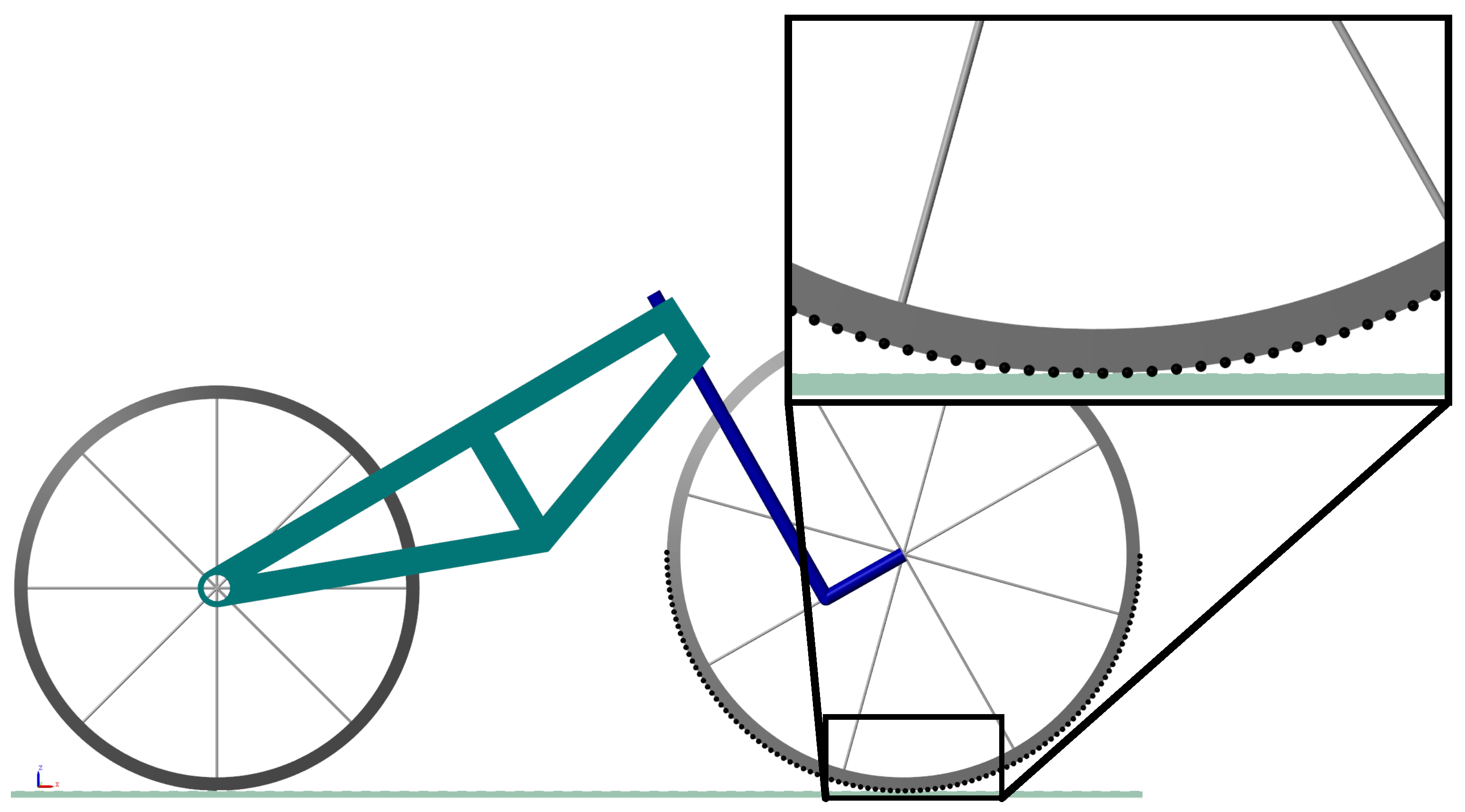
2.1. System Multibody Model

The two-wheeled vehicle of interest for this research work is modeled as a multibody system composed of the following four rigid bodies:
  • The rear wheel.
  • The rear frame.
  • The front fork/handlebars.
  • The front wheel.
Three revolute joints keep the system assembled while it moves freely on the horizontal plane. The permanent contact constraint between each wheel and the plane is also considered. The first revolute joint links the rear wheel and the rear frame. Perpendicular to this, a second revolute joint allows the steering of the front fork/handlebars. Finally, a third revolute joint allows the rotation of the front wheel with respect to the fork/handlebars. The horizontal road plane is contained by the XY axes of the inertial reference frame. Therefore, the multibody system model of the two-wheeled vehicle considered herein has a seven-dimensional configuration space, as discussed in detail below.

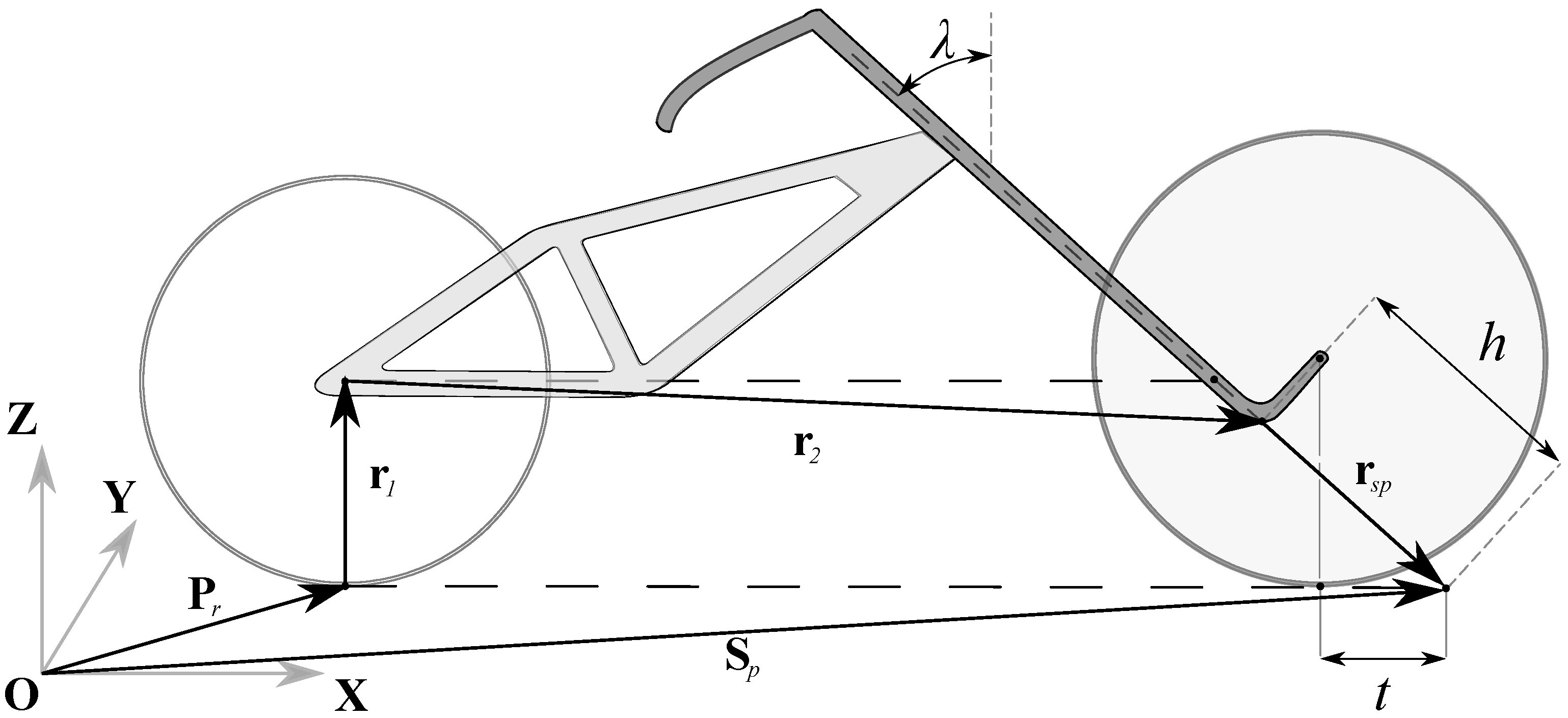
2.2. System Geometry

The geometry of the system under consideration is shown in Figure 1.
The geometric model includes the set of standard geometric parameters used to describe two-wheeled vehicles. These are defined for the system configuration with a zero steering angle and considering an upright position on a horizontal plane. This set of parameters is defined as follows:
  • The distance between the contact points of the rear and front wheel, known as wheelbase and denoted with c w .
  • The distance between the front contact point and the steering column intersection with the road plane, known as trail and denoted with t.
  • The rear and front wheels radii respectively denoted with a r and a f .
  • The tilt angle of the steering column, known as the caster angle and denoted with λ .
Besides, three additional parameters are used to simplify the kinematic analysis. These are defined as functions of the standard geometrical parameters, as respectively shown in Equations (1)–(3).
d = a f sin λ t cos λ
L = c w + t a r tan ( λ )
H = a f a r d sin ( λ ) cos ( λ )
The fork offset denoted with d is the minimum distance between the center of the front wheel and the steering column. In addition, the auxiliary parameters L and H can be geometrically interpreted from Figure 1 since they serve to complete the geometric description of the model. This process allows for obtaining a schematization of the system geometry in a simplified skeleton, as shown in Figure 2.

2.3. Kinematic Analysis

With the geometry defined, the reference frames and the coordinates vector are now considered. The horizontal road plane is defined by the X and Y axes of the global reference frame OXYZ . Its Z axis direction is opposed to the gravity. Three additional local reference frames are used to describe the orientation of the multibody system, as shown in Figure 3.
The reference frame O 1 X 1 Y 1 Z 1 is fixed on the contact point between the rear wheel and the road plane. The position vector of its origin is defined as
P r = X r Y r 0 T
where X r and Y r are the coordinates of the contact point on the ground considering the X and Y axes of the global reference frame. The orientation of the local reference frame O 1 X 1 Y 1 Z 1 is given by the transformation matrix obtained by two successive rotations. That is, the yaw of the rear wheel is given by the angle θ , and the roll is associated with the angle χ . Therefore, its orientation is independent of the rotation of the wheel. The transformation matrix is defined as follows
A 1 , 0 = R z θ R x χ
where the generic rotation matrix A i , 0 represents the transformation matrix between the local reference system labeled with i, that is associated with the generic rigid body i, and the global reference system labeled with 0. Subsequently, one can define the reference frame O 2 X 2 Y 2 Z 2 , whose origin is fixed to the center of the rear wheel and its orientation is given by the yaw angle θ , the roll angle χ , and the pitch angle μ of the rear frame, having the following transformation matrix
A 2 , 0 = A 1 , 0 R y μ
Then, the origin of the reference frame O 3 X 3 Y 3 Z 3 is fixed at the location shown in Figure 3, and its orientation is given by
A 3 , 0 = A 2 , 0 R y T ( λ ) R z ( ψ )
where the caster angle λ was considered in the rotation matrix R y T ( λ ) in order to have positive values for a backward tilt of the steering column. In summary, the vector of Lagrangian coordinates employed to define the spatial configuration of the multibody system that models the two-wheeled vehicle is
q = X r Y r θ χ μ ψ ϕ r ϕ f T
where X r and Y r respectively represent the X and Y coordinates of the rear wheel contact point, θ is the yaw angle of the rear assembly (rear wheel and rear frame), χ is the roll angle of the rear assembly, μ is the pitch angle of the rear frame, ψ is the steering angle of the front fork/handlebars, while ϕ r and ϕ f are the angular displacements due to the rotation of the rear and front wheels, respectively.

2.4. System Kinematic Chain

A kinematic model based on a closed chain is proposed to study the two-wheeled vehicle kinematics, as shown in Figure 4.
The kinematic chain can be directly written by using a vector approach as
P r + r 1 + r 2 + r 3 + r 4 = P f
In the following, the components of the kinematic chain are described in detail. The points P r and P f respectively identify the position vectors of the contact points of the rear and front wheel with the road plane, which have their Cartesian components given by the following expressions
P r = X r Y r 0 T
P f = X f Y f 0 T
The vector r 1 , starting from the contact point P r to the center of the rear wheel, can be expressed in the global coordinates of the reference frame O 1 X 1 Y 1 Z 1 as
r 1 = A 1 , 0 0 0 a r = a r sin χ sin θ a r sin χ cos θ a r cos χ
Subsequently, the vector r 2 , defined in the reference frame O 2 X 2 Y 2 Z 2 with its tail located on the rear wheel center and its head on the point O 3 , in global coordinates is equal to
r 2 = A 2 , 0 L H s λ 0 H c λ = L H s λ c μ c θ s χ s μ s θ + H c λ c θ s μ + c μ s χ s θ L H s λ c μ s θ + s χ c θ s μ + H c λ s μ s θ c μ s χ c θ c χ L s μ H c λ μ
Then, the vector r 3 having its tail fixed at the point O 3 and its head located at the center of the front wheel, in global coordinates is written as
r 3 = A 3 , 0 d 0 0 = d c ψ c θ c λ μ + s λ μ s χ s θ     d c χ s ψ s θ d c ψ s θ c λ μ s λ μ s χ c θ   +   d c χ c θ s ψ d s χ s ψ + s λ μ c χ c ψ
Finally, two methodologies are studied to write the expression for the position vector r 4 , which has its tail fixed on the geometric center of the front wheel and its head located at the instantaneous contact point of the front wheel denoted with P f . Each of these methodologies yields a different set of kinematic constraint equations. Therefore, two different kinematic models are proposed in the present work, as described in detail below.

2.5. Cross-Product Model

An effective approach for mathematically formulating the geometric vector denoted with r 4 consists of determining the direction of the said vector in the global reference frame, as explained in detail in the following derivations. The unit vector normal to the plane of symmetry of the front wheel can be written in global coordinates as
n ^ 4 = A 3 , 0 0 1 0 = s ψ c θ c λ μ + s λ μ s χ s θ     c χ c ψ s θ c χ c ψ c θ s ψ s θ c λ μ s λ μ s χ c θ c ψ s χ s λ μ c χ s ψ
Then, the unit vector tangent to the front wheel at the contact point can be written as
t ^ 4 = n ^ 4 × K ^ n ^ 4 × K ^ = c χ c ψ c θ     s ψ s θ c λ μ   +   s λ μ s χ c θ s ψ s λ μ 2 s χ 2 s ψ 2   +   2 s λ μ c χ c ψ s χ s ψ   +   c χ 2 c ψ 2   +   s ψ 2 c λ μ 2 c θ s ψ c λ μ   +   c χ c ψ s θ   +   s λ μ s χ s ψ s θ s λ μ 2 s χ 2 s ψ 2   +   2 s λ μ c χ c ψ s χ s ψ   +   c χ 2 c ψ 2   +   s ψ 2 c λ μ 2 0
where K ^ = 0 0 1 T is a constant unit vector opposite to the direction of the gravity acceleration and normal to the road plane. It can be proved that the Z component of the tangent unit vector t ^ 4 is equal to zero. This is a consequence of the fact that the vector t ^ 4 must be tangent to the XY plane. Finally, the vector r 4 can be written as
r 4 , c = a f n ^ 4 × t ^ 4 = a f c ψ s χ     s λ μ c χ s ψ c θ s ψ c λ μ   +   c χ c ψ s θ   +   s λ μ s χ s ψ s θ s λ μ 2 s χ 2 s ψ 2   +   2 s λ μ c χ c ψ s χ s ψ   +   c χ 2 c ψ 2   +   s ψ 2 c λ μ 2 a f c ψ s χ     s λ μ c χ s ψ c χ c ψ c θ     s ψ s θ c λ μ   +   s λ μ s χ c θ s ψ s λ μ 2 s χ 2 s ψ 2   +   2 s λ μ c χ c ψ s χ s ψ   +   c χ 2 c ψ 2   +   s ψ 2 c λ μ 2 a f c χ 2 c ψ 2 c λ μ 2   +   2 c χ 2 c ψ 2   +   c χ 2 c λ μ 2     c χ 2   +   2 s λ μ s χ s ψ c χ c ψ     c ψ 2   +   1 s λ μ 2 s χ 2 s ψ 2   +   2 s λ μ c χ c ψ s χ s ψ   +   c χ 2 c ψ 2   +   s ψ 2 c λ μ 2
where the subscript c in r 4 , c indicates that the cross-product approach has been used in the geometric determination of this vector. Since n ^ 4 and t ^ 4 are mutually perpendicular unit vectors, the magnitude of the vector r 4 , c is imposed equal to the radius of the front wheel. Each of the vectors computed so far is shown in Figure 5, from which the geometric interpretation of the present formulation approach can be visualized.
With the components of the kinematic chain defined as described above, a closed-loop vector equation can be written as follows
P f P r = r 1 + r 2 + r 3 + r 4 , c
Then, due to the continuous contact with the road plane, this expression must satisfy the following constraint
K ^ T P f P r = 0
where, considering Equations (12)–(14) and (17), the fundamental equation for modeling the contact condition assumes the following form
d s χ s ψ + s λ μ c χ c ψ   +   a r c χ c χ s μ L H s λ   +   H c χ c λ c μ a f c χ 2 c ψ 2 c λ μ 2   +   2 c χ 2 c ψ 2   +   c χ 2 c λ μ 2     c χ 2   +   2 s λ μ s χ s ψ c χ c ψ     c ψ 2   +   1 s λ μ 2 s χ 2 s ψ 2   +   2 s λ μ c χ c ψ s χ s ψ   +   c χ 2 c ψ 2   +   s ψ 2 c λ μ 2 = 0
Additionally, the X and Y components of Equation (18) are given as follows
X f X r = L H s λ c μ c θ s χ s μ s θ   +   + H c λ c θ s μ + c μ s χ s θ   +   d c ψ c θ c λ μ + s λ μ s χ s θ     c χ s ψ s θ   +   a r s χ s θ     a f c ψ s χ s λ μ c χ s ψ c θ s ψ c λ μ   +   c χ c ψ s θ   +   s λ μ s χ s ψ s θ s λ μ 2 s χ 2 s ψ 2   +   2 s λ μ c χ c ψ s χ s ψ   +   c χ 2 c ψ 2   +   s ψ 2 c λ μ 2
Y f Y r = L H s λ c μ s θ + s χ c θ s μ   +   H c λ s μ s θ c μ s χ c θ   +   d c ψ s θ c λ μ s λ μ s χ c θ   +   c χ c θ s ψ     a r s χ c θ   +   a f c ψ s χ     s λ μ c χ s ψ c χ c ψ c θ     s ψ s θ c λ μ   +   s λ μ s χ c θ s ψ s λ μ 2 s χ 2 s ψ 2   +   2 s λ μ c χ c ψ s χ s ψ   +   c χ 2 c ψ 2   +   s ψ 2 c λ μ 2
As will be discussed in detail in the presentation of the numerical results, Equations (20)–(22) allow for fully defining the kinematic configuration of the two-wheeled vehicle system for a set of values of its degrees of freedom. In particular, these expressions are useful to study the behavior of the rear frame pitch angle denoted with μ . Also, the current approach leads to the analytical determination of the relative displacement of the contact points of the wheels as functions of the system degrees of freedom.

2.6. Surface Parametrization Model

An alternative approach to formulate a consistent analytical expression for the vector r 4 focuses on noting that, when a set of changes in the degrees of freedom takes place, this fundamental vector experiences an angular displacement in the local reference frame O 3 X 3 Y 3 Z 3 . This phenomenon can be modeled by introducing an additional geometric variable that serves as a non-generalized coordinate, that is, an angular position coordinate of a massless point that plays the role of an auxiliary geometric parameter. Therefore, the vector of Lagrangian coordinates, when employing this approach, assumes the following different form
q s = X r Y r θ χ μ ψ ϕ r ϕ f β T
where β denotes the non-generalized coordinate which identifies the angular position of the contact point in the local reference frame, as shown in Figure 6a for the system in the initial configuration and in Figure 6b in the case of an arbitrary configuration.
In both cases considered in Figure 6, the angles of rotation of the rear and front wheel, which are respectively denoted with ϕ r and ϕ f , are set equal to zero. Thus, only changes in the coordinates χ , ψ , and μ take place in these scenarios. In fact, as it will be shown later in the paper by means of numerical experiments, the angular displacement β is not a function of the angle ϕ f . The coordinate β allows for analytically expressing the geometric vector r 4 as follows
r 4 , s = A 3 , 0 a f cos β 0 a f sin β T
where the subscript s in the vector term r 4 , s indicates that the surface parametrization approach was used. Subsequently, the vector tangent to the wheel at the point of contact is obtained by partially differentiating Equation (24) with respect to the non-generalized angular displacement β . This vector has the form
t 4 = r 4 β = a f c β s λ μ c θ s χ s θ c λ μ s β c ψ c θ c λ μ + s λ μ s χ s θ     c χ s ψ s θ     c β s λ μ s θ + s χ c θ c λ μ s β c ψ s θ c λ μ s λ μ s χ c θ   +   c χ c θ s ψ c β c χ c λ μ s β s χ s ψ + s λ μ c χ c ψ
Then, a constraint equation can be written by considering that this vector must be perpendicular to the unit vector normal to the road plane denoted with K ^ . Therefore, one can write:
K ^ T t 4 = 0
By doing so, the following constraint equation is obtained
s β s χ s ψ + s λ μ c χ c ψ     c β c χ c λ μ = 0
It is worth mentioning that, given the non-linearity of Equation (27), to obtain an explicit expression for the angle β without resorting to approximations, being this the common path in the literature, it is not a trivial task. However, in the present work, the fully nonlinear expression will be considered. When all the components of the kinematic chain are defined, a closed-loop is proposed, as previously done with the cross-product model. Again, the vector equation associated with the closure of the geometric loop can be written as follows
P f P r = r 1 + r 2 + r 3 + r 4 , s
Thus, the contact condition of the wheels, as formulated in Equation (19), yields the second kinematic constraint of the surface parametrized model given by
d s χ s ψ + s λ μ c χ c ψ   +   a r c χ + a f c β s χ s ψ + s λ μ c χ c ψ     c χ s μ L H s λ   +   H c χ c λ c μ + a f c χ s β c λ μ = 0
Finally, the X and Y components of Equation (28) are equal to
X f X r = d c ψ c θ c λ μ + s λ μ s χ s θ     c χ s ψ s θ   +   H c λ c θ s μ + c μ s χ s θ   +   a f c β c ψ c θ c λ μ + s λ μ s χ s θ     c χ s ψ s θ   +   a r s χ s θ     a f s β s λ μ c θ s χ s θ c λ μ   +   L H s λ c μ c θ s χ s μ s θ
Y f Y r = d c ψ s θ c λ μ s λ μ s χ c θ   +   c χ c θ s ψ   +   H c λ s μ s θ c μ s χ c θ   +   a f c β c ψ s θ c λ μ s λ μ s χ c θ   +   c χ c θ s ψ     a r s χ c θ     a f s β s λ μ s θ + s χ c θ c λ μ   +   L H s λ c μ s θ + s χ c θ s μ
The set of Equations (27), (29)–(31) allows for studying the kinematics of the two-wheeled vehicle system in detail. In particular, when consistent values are assigned to the degrees of freedom of the multibody system, the displacement of the contact point of the front wheel, defined relative to that of the rear wheel, can be readily determined.

2.7. Steering Point Kinematics

As shown in Figure 7, the point in the road plane created by the projection of the steering axis is named the steering point.
This is also a geometric parameter of interest for the mechanical design, as it can provide insight into the kinematics of two-wheeled vehicles in general. Specifically, the magnitude obtained from the expression S P P f , known as the mechanical trail, is also studied for its influence on the system stability [66]. On the other hand, the trajectory of the steering point is studied here, whose position vector is written as a function of the system generalized coordinates as follows
S P = P r + r 1 + r 2 + r s p = P r + r 1 + r 2 + A 3 , 0 0 0 h
where the term h in Equation (32) represents the distance from the point O 3 to the steering point expressed in local coordinates. This is found by noting that the Z component of the steering point in global coordinates must be equal to zero. Thus, this consideration yields the following expression
h = a r L sin μ   +   H cos λ μ cos λ μ
By back-substituting Equation (33) into Equation (32), the steering point position vector can be written as
S P = X r + cos θ L cos λ   +   a r sin λ     μ cos λ     μ Y r + sin θ L cos λ   +   a r sin λ     μ cos λ     μ 0
From this expression, it can be observed that, given a null yaw angle denoted with θ and when arbitrarily changing the steering angle denoted with ψ , the displacement of the steering point is not zero only in the X component of the system global reference frame.

2.8. Front Assembly Orientation

Due to the method employed to formulate the transformation matrix of the front assembly, the set of Euler angles describing the orientation of such subsystem are not explicitly known. However, these angles can be obtained from the components of the matrix presented in Equation (7) by noting that three successive rotations can fully describe the orientation of the front frame assembly. In particular, this can be done by considering a set of Euler angles based on the sequence Z-X-Y as follows
à 3 , 0 = c ϕ c δ s α s ϕ s δ c α s δ c δ s ϕ + c ϕ s α s δ c ϕ s δ + s α c δ s ϕ c α c δ s ϕ s δ c ϕ s α c δ c α s ϕ s α c α c ϕ
where δ , α , and ϕ represent the absolute yaw, roll, and pitch angles of the front frame, respectively. The explicit expressions for these geometric quantities, as functions of the generalized coordinates, can be obtained by equating the components of Equation (Section 2.8) with those of the matrix reported in Equation (7). For instance, the angle α can be obtained as
A 3 , 0 3 , 2 = Ã 3 , 0 3 , 2
which leads to
sin α   =   cos ψ sin χ     sin λ μ cos χ sin ψ
An explicit expression for the camber angle as a function of the generalized coordinates results valuable when considering tire models for two-wheeled vehicles [67,68]. In particular, for computing the tire lateral force, which strongly depends on this parameter, the determination of the camber angle represents a fundamental geometric task which must be fully addressed preliminarily to the dynamic analysis. Similarly, the equation for computing the yaw angle of the front assembly denoted with δ can be formulated as follows
A 3 , 0 1 , 2 = Ã 3 , 0 1 , 2
which leads to
sin δ = sin ψ cos θ cos λ     μ   +   sin λ     μ sin χ sin θ cos α   +   cos χ cos ψ sin θ cos α
and
A 3 , 0 2 , 2 = Ã 3 , 0 2 , 2
which leads to
cos δ = sin ψ sin θ cos λ     μ     sin λ     μ sin χ cos θ cos α   +   cos χ cos ψ cos θ cos α
Finally, the pitch angle of the front assembly denoted with ϕ can be expressed as a function of the system generalized coordinates as follows
A 3 , 0 3 , 1 = Ã 3 , 0 3 , 1
which leads to
sin ϕ = sin χ sin ψ   +   sin λ μ cos χ cos ψ cos α
and
A 3 , 0 3 , 3 = Ã 3 , 0 3 , 3
which leads to
cos ϕ = cos χ cos λ μ cos α
Equations (37), (39), (41), (43) and (45) allow for explicitly defining the orientation of the front assembly of the complete multibody system and can be useful for further modeling tasks in the kinematic and dynamic analysis of two-wheeled vehicles.

3. Numerical Results and Discussion

In this section, a set of numerical experiments is proposed to study the kinematic models developed in this investigation, namely, the two-wheeled vehicle models arising from the use of the cross-product method and the surface parametrization approach. Besides, three additional two-wheeled vehicle models are considered to confront the numerical results found. In particular, two of these kinematic models used for making comparisons are found the literature [59,60], while the third model represents a detailed multibody model created by the authors using the SIMSCAPE MULTIBODY software implemented in the MATLAB computational environment.
The remainder part of this section is organized as follows. Section 3.1 provides a detailed description of the numerical experiments proposed, as well as the numerical values of the physical parameters employed in the two-wheeled vehicle models. Section 3.2 reports the numerical experiment results and the comparative metrics calculated with respect to the model results obtained considering the two-wheeled vehicle model developed using the SIMSCAPE MULTIBODY software. Finally, Section 3.3 provides some final remarks and a detailed discussion on the numerical results found.

3.1. Description of the Numerical Experiments

The purpose and scope of the numerical experiments proposed in this section are to study the system kinematic configuration, employ a kinematically driven approach, and compare the numerical results obtained from this study with those calculated using the kinematic models available in the literature. To this end, in order to implement a kinematically driven approach, the first step consists of analyzing the behavior of the system redundant coordinates when the set of the known values of the degrees of freedom are changed. This is equivalent to analyze the system kinematic constraints, being, in general, these nonlinear algebraic equations among the most complex features in modeling two-wheeled vehicles. In particular, the main goal is to study and understand the relationship between the roll angles of the steering and rear frames with the remaining kinematic variables, primarily resulting from the manipulation of the redundant coordinates in correspondence of the enforcement of the contact between the vehicle wheels and the road. That is, one fundamental objective is to derive the kinematic relationship between the pitch angle μ and the migration angle β associated with the contact point of the front wheel. Similarly, it is of interest for this research to analyze the behavior of the Euler angles of the front assembly when a consistent change in the values of the degrees of freedom is performed. This last kinematic problem does not represent a straightforward task, but it can be readily solved by employing the explicit kinematic expressions found in the present work.
Two-wheeled vehicles are underactuated multibody mechanical systems, which means that the number of external control inputs is less than the number of the system degrees of freedom. Consequently, their complex dynamic behavior cannot be fully described only with a kinematic model, requiring further development of a suitable dynamic model. Besides, if the no-slip condition between the wheels and the ground is considered, although the occupiable regions of the position space remain unaffected, these systems have four nonholonomic constraints and three degrees of freedom in the velocity space [69]. However, the accessible configuration space of the model is still seven-dimensional, as mentioned before. Therefore, to study this family of systems with a kinematically driven approach, seven independent coordinates must be known. For this purpose, it is defined the vector q m i n with a chosen set of independent coordinates as follows
q m i n = X r Y r θ χ ψ ϕ r ϕ f T
where, as already mentioned in the manuscript, X r and Y r represent the Cartesian coordinates of the contact point collocated on the rear wheel, θ and χ respectively denote the yaw angle and the roll angle of the rear assembly, composed of the rear wheel and the rear frame, ψ represents the steering angle of the handlebars, while the angular displacements denoted with ϕ r and ϕ f are respectively associated with the rotation of the rear and front wheels about their axes. Thus, for a known vector of generalized coordinates q m i n , the kinematic constraints of the model can be numerically solved, leading to appropriate values of the redundant coordinates. In particular, the kinematically driven analysis employed in this work for the model proposed in Section 2.5, namely the cross-product model, consists of the following fundamental steps:
  • Substitute the components of the given vector q m i n into Equation (20).
  • Solve numerically this algebraic equation to find the corresponding value of the angle μ employing the Newton-Raphson method considering an initial estimation μ 0 = 0 (rad) and an appropriate small tolerance denoted with ϵ .
  • Input the now known vector of Lagrangian coordinates of Equation (8) into Equations (21) and (22) to compute the relative Cartesian coordinates of the contact point of the front wheel.
  • Input the vector of Lagrangian coordinates into the explicit expressions given in Equations (37), (39), (41), (43) and (45) for computing the Euler angles of the front assembly.
On the other hand, the surface parametrization model, defined in Section 2.6, includes two kinematic constraints defined in Equations (27) and (29), respectively. Therefore, its augmented vector of Lagrangian coordinates defined in Equation (23) has an additional non-generalized coordinate denoted with β to account for the angular migration of the contact point on the front wheel. Thus, the kinematically driven analysis of the parametrized surface model is summarized as follows
  • Substitute the components of the given vector of Lagrangian coordinates q m i n into Equations (27) and (29).
  • Solve the set of nonlinear equations resulting from the previous step using the Newton-Raphson method considering the initial estimations μ 0 = 0 (rad) and β 0 = λ (rad), as well as a sufficiently small tolerance denoted with ϵ .
  • Use the now known Lagrangian coordinate vector q s of the kinematic model to calculate the relative Cartesian coordinates of the front contact point by substituting it into Equations (30) and (31).
In the set of numerical experiments considered in this work, the numerical results of two additional models found in the literature are included to confront the behavior of the proposed analytical approaches. Besides, an additional kinematic model, developed by the authors based on the SIMSCAPE MULTIBODY toolbox belonging to the MATLAB multi-paradigm programming platform, is used as a reference for comparing and validating all the numerical results found in this work. To this end, a performance index based on the Root-Mean-Squared Error (RMSE) is employed as a quantitative metric useful for making consistent comparisons. This index is computed as follows
R M S E = 1 N i = 1 N y i y ^ i 2
where N is the number of data, y i is the reference value, and y ^ i is the experimental data. Figure 8 shows a graphical visualization of the SIMSCAPE MULTIBODY model employed in this work as a reference model.
Figure 8 includes a zoom in the region of contact of the front wheel with the road plane. This shows the approach used to identify the instantaneous point of contact, measure its migration angle β , and define its global position vector P f . In general, the software SIMSCAPE MULTIBODY allows for performing measurements of the kinematic variables of the rigid bodies defined in the dynamical simulation. However, there is a software limitation of its measurement capacity related to the existence of contact points between rigid bodies. In fact, it is only possible to carry out measurements in the centers of mass or fixed local reference frames of two bodies in contact. However, no information regarding the location of the instant contact point can be obtained directly. Therefore, as a workaround for these software limitations, a very large number of contact proxies were created along the perimeter of the front wheel within the range β = [ 85 , 85 ] (deg), that is, N c = 1000 , where N c denotes the number of contact nodes. By doing so, the instantaneous point of contact is identified by the simultaneous measurement of the normal force of the created proxies. In this way, the migration angle measurement is discretized using a fine grid with multiples of 0.003 (deg). Regarding the orientation angles of the front assembly, on the other hand, SIMSCAPE MULTIBODY allows the direct measurement of numerical values of the transformation matrices associated with each rigid body. Consequently, by implementing a numerical procedure similar to the one described in Section 2.8, these values can be indirectly calculated. Furthermore, the numerical values of the parameters employed for the numerical experiments are reported in Table 1.
The numerical values of the physical parameters reported in Table 1 are consistently used to evaluate the five kinematic models considered in this investigation, namely the SIMSCAPE MULTIBODY kinematic model, the cross-product kinematic model, the surface parameterization kinematic model, the Cossalter kinematic model [60], and the Frosali and Ricci kinematic model [59]. Furthermore, to carry out a consistent comparison, one should note that there is a discrepancy in the conventions for defining the reference frames employed in the kinematic models proposed in [59,60], and these differences should be carefully accounted for in the confront. For the benefit of the interested reader, the key equations of the kinematic models proposed in [59,60] are reported in Appendix A. For this reason, the kinematically driven analysis previously described is carried out for a full rotation of the handlebars of the two-wheeled vehicle models. Thus, the steering angle is varied between [ 0 , 360 ] (deg). Additionally, two values of the roll angle of the rear frame, namely [ 0 , 15 ] (deg), are considered. Besides, the coordinates X r , Y r , and θ are set to zero during the numerical experiments to simplify the comparison. This is possible because these three generalized coordinates are of interest only to define the system position with respect to the inertial reference frame, but do not influence the relative configuration of the front assembly or the constraint of permanent contact of the wheels with the road. These assumptions on the measures derived from the numerical experiments make it possible to simplify the adaptations required in the results due to discrepancies in the definition of the reference frames mentioned above.

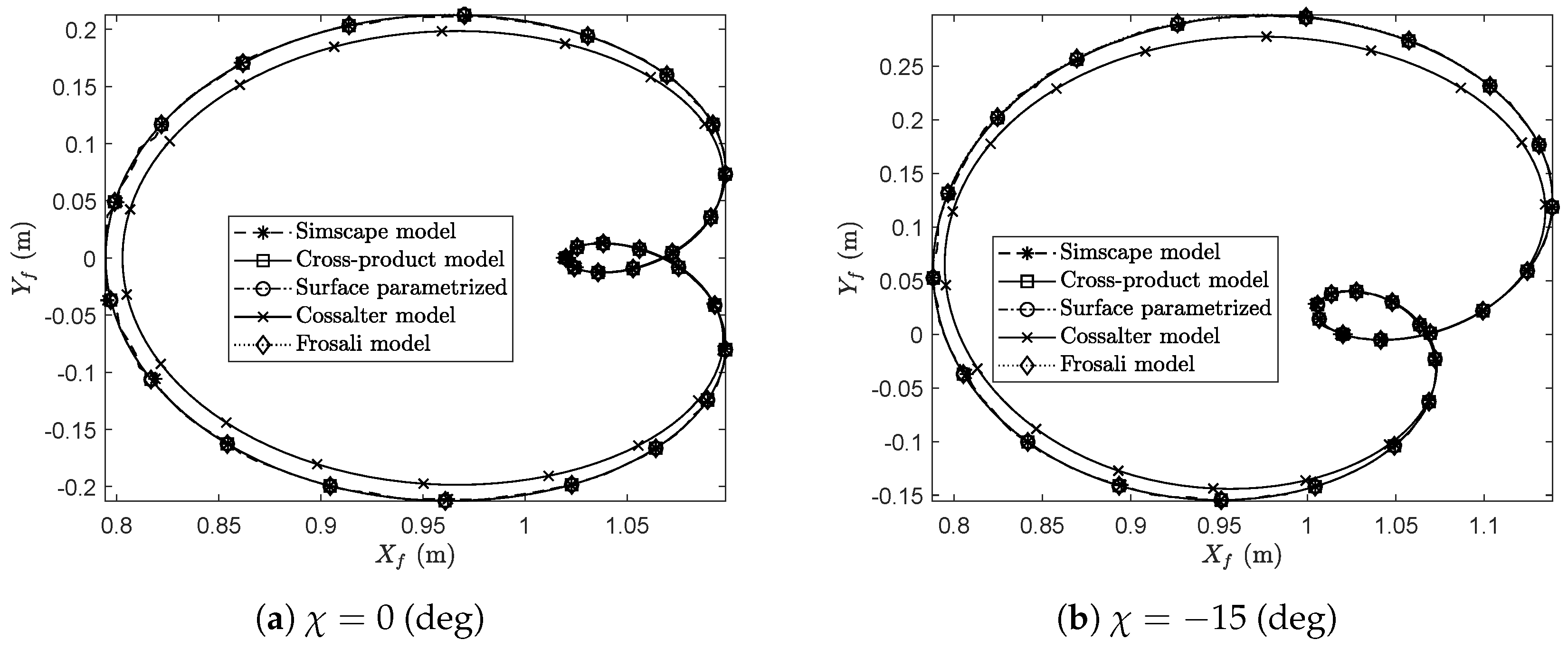
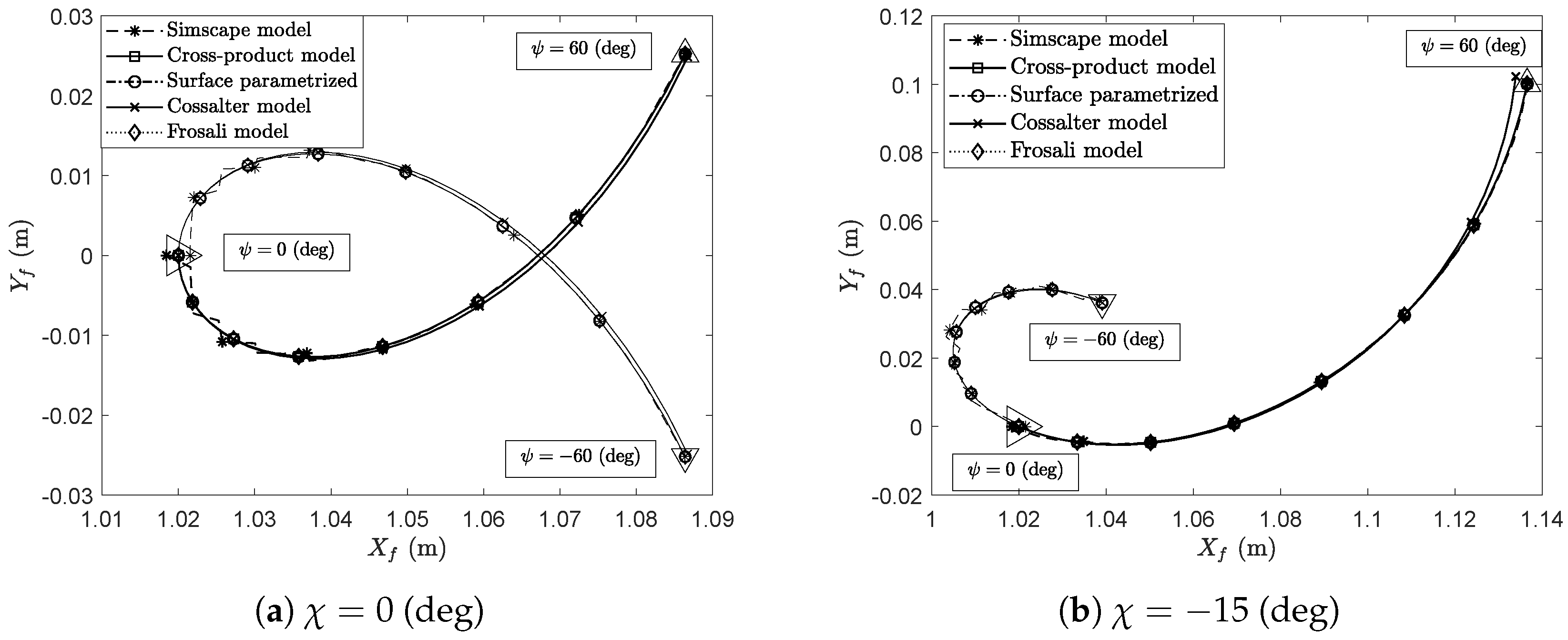
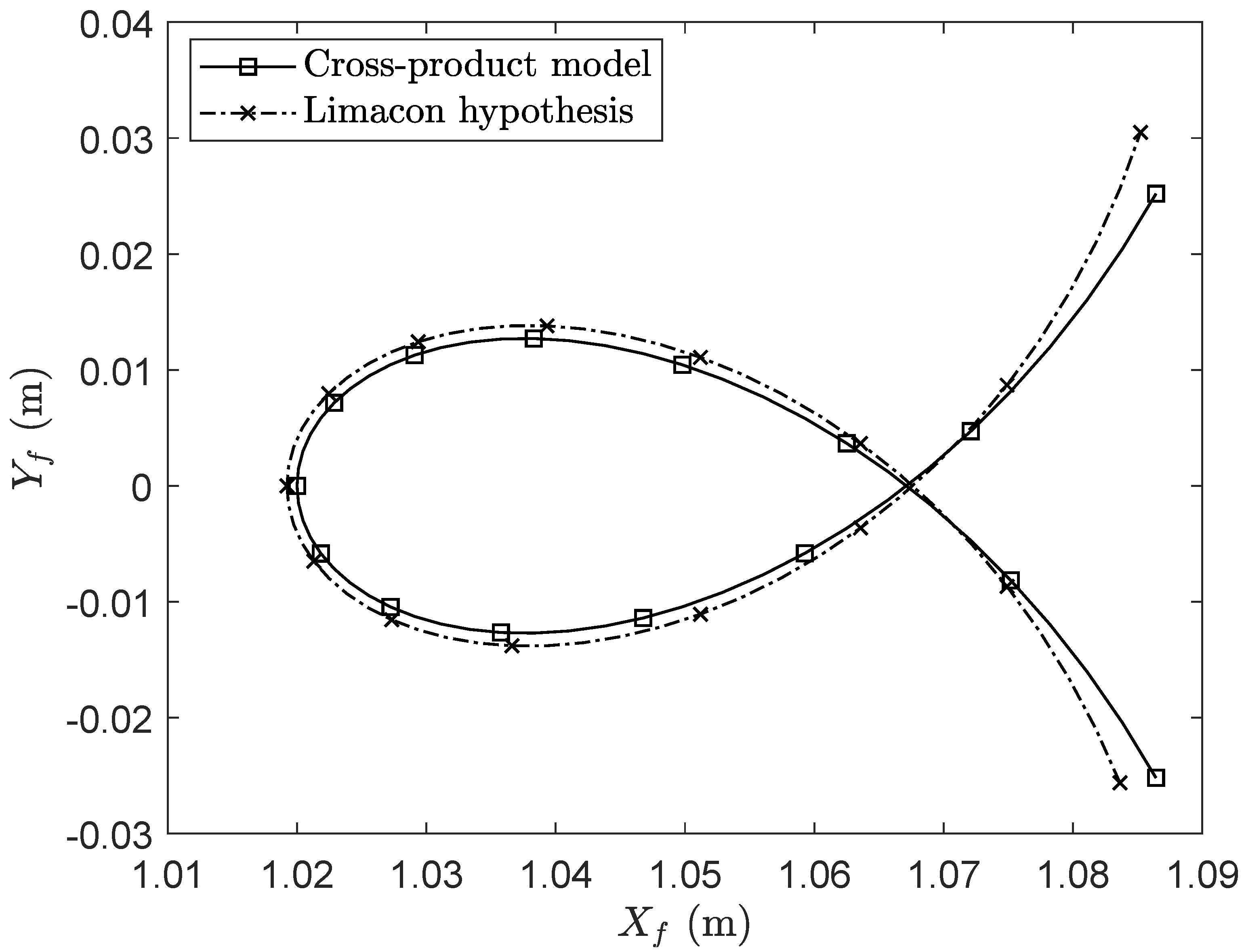
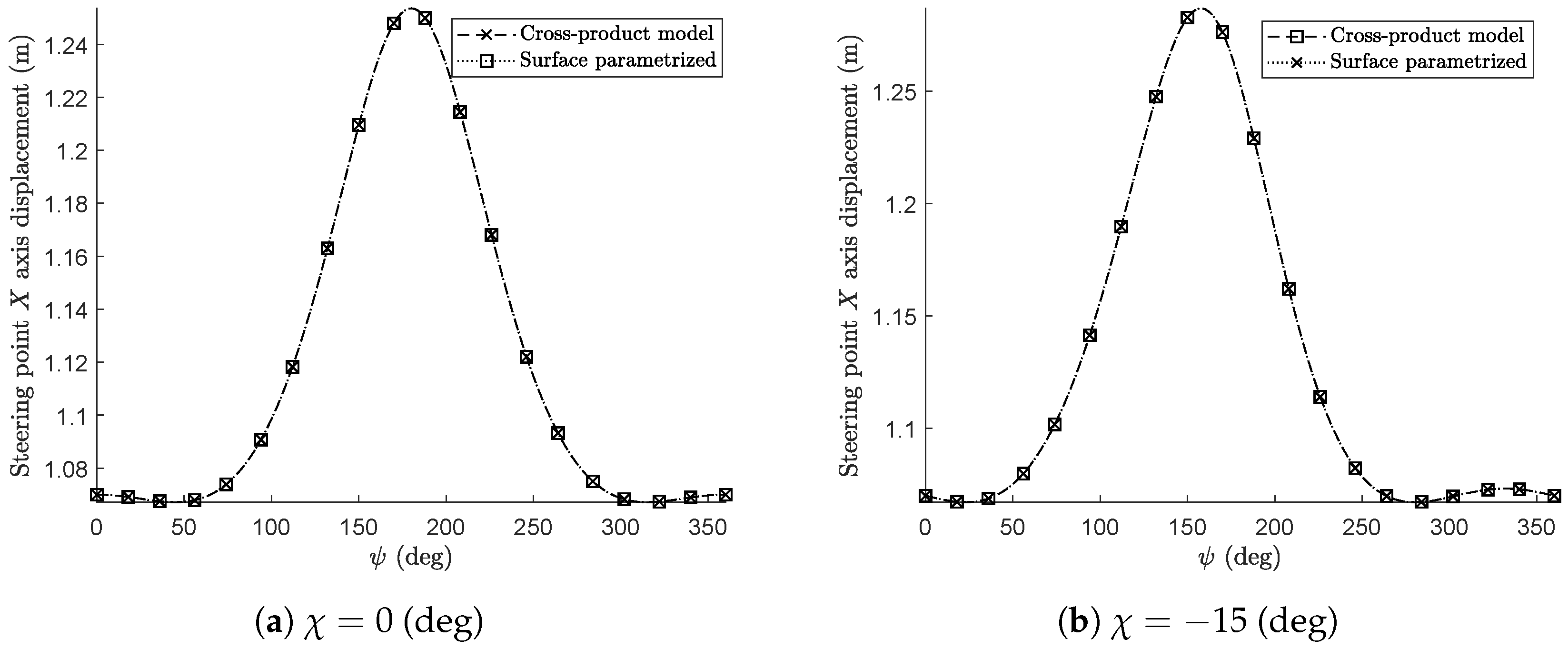
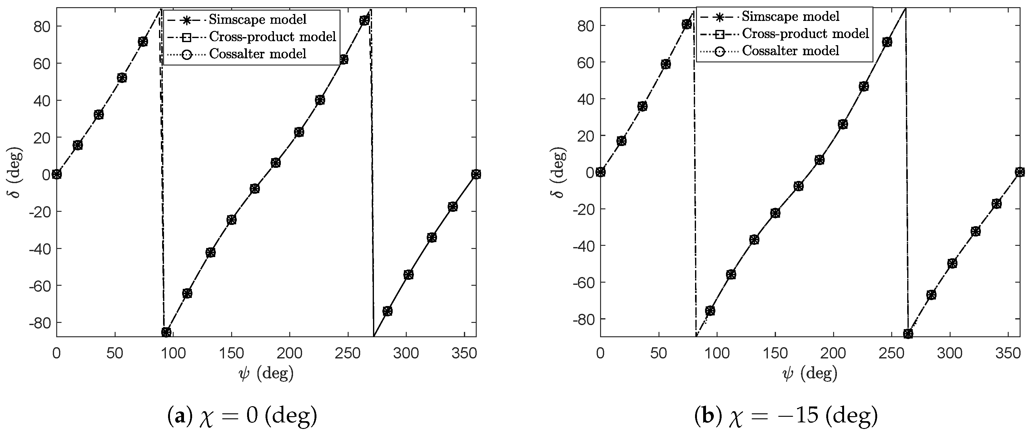
3.2. Kinematically Driven Study and Comparative Analysis

In this subsection, the numerical results of the kinematically driven study and the corresponding comparative analysis developed in this work are presented. More specifically, the first part of this subsection is devoted to the comparative analysis of the trajectory followed by the contact point belonging to the front wheel, while the second part of this subsection focuses on the study of the set of Euler angles representing the orientation of the front assembly.
The trajectory described by the point of contact of the front wheel on the road plane, given a full rotation of the the handlebars, is shown in Figure 9.
For a zero roll angle, it is observed that the trajectory is symmetric about the X axis, as shown in Figure 9a. This not being the case when the roll angle is equal to −15 (deg), as evidenced in Figure 9b. In particular, restricting the plotting of the numerical results within the range of the steering angle ψ = [ 60 , 60 ] (deg) produces the graphical representation depicted in Figure 10.
Within this interval, considering a null roll angle, 21.9 % of the total trajectory range is covered on the X axis, while 11.8 % results on the Y axis. In contrast, having a fixed roll angle equal to 15 (deg) increases the covered range to 37.6 % and 23.3 % in the X and Y axis, respectively. In Figure 10a,b, the marker ▷ represents the position of the contact point when the steering angle is zero. Also, in Figure 10a,b, the markers ▽ and indicate the points corresponding to 60 (deg) and 60 (deg), respectively.
Given the geometry of the trajectory described by the front wheel contact point, it is of interest to study its similarity with a looped line that is mathematically described by the Limacon curve. Such comparison is presented in Figure 11.
The Limacon curve is described in polar coordinates by the following equation
r = a b cos ψ
where r represents the radial distance of a generic point on the Limacon curve, measured from a reference point set equal to the origin of the global reference system, and ψ denotes the angular displacement from a reference direction associated with the horizontal axis, while the constants a and b define the aspect ratio of the inner loop of the curve. This parametric curve is equivalently described in Cartesian coordinates as follows
r = ξ + cos ψ + φ a b cos ψ η + sin ψ + φ a b cos ψ
where ξ and η respectively represent the offset in X and Y axes, while the parameter φ accounts for the rotation of the entire curve with respect to the global reference frame. The numerical values of these parameters are found by performing a numerical optimization using the MATLAB built-in function fmincon. To this end, the goal is to minimize the following objective function subjected to a proper set of constraints
min x ^ x 2 + y ^ y 2 subject to : a 0 b 0 a b
where x ^ and y ^ are the vectors of numerical results of the cross-product model, and x and y are the vectors calculated with the use of Equation (49). In addition, the proposed set of algebraic constraints guarantee the existence of the inner loop that characterizes the geometry of the trajectory described by the contact point of the front wheel. For the particular case study considered herein, the optimized numerical values of the parameters are a = 0.1188 , b = 0.1672 , φ = 1.7370 × 10 10 , ξ = 1.0676 , and η = 7.2167 × 10 11 . These parameters yield a minimized value of the objective function equal to 1.2650 × 10 4 within the interval ψ = [ 60 , 60 ] (deg).
Figure 12 shows the behavior of the non-generalized parameter β when the handlebars is fully rotated.
In the cross-product model, the vector r 4 , c in Equation (17) is defined a priori in the global coordinate system. Therefore, one does not have an explicit expression for the geometric parameter β . However, it is found that the third Euler angle of the front assembly, defined in Equations (43) and (45), is closely related to the angular displacement β . In particular, the numerical values reported in Figure 12 using the cross-product model have been obtained by the following equation
tan β = tan ϕ
This expression is obtained from Equations (27), (43) and (45). The results from the numerical approach with the surface parametrized model show a very good agreement. In particular, after considering an offset equal to λ , the plot in Figure 12 for the surface parametrized model is produced. For the entire rotation of the handlebars, the angle β has a range of 69.4912 (deg) given a null roll angle, and 76.4907 (deg) when the roll angle is equal to 15 (deg). In contrast, when restricting the angular displacement ψ within the interval [ 60 , 60 ] (deg), the ranges of variation of the geometric parameter β are 13.9493 (deg) for a null roll angle and 28.3808 (deg) for a roll angle equal 15 (deg), respectively. Based on this behavior, the assumption that the front wheel contact point is contained in the symmetry plane of the rear frame, which is equivalent to assuming a null non-generalized coordinate β , is very frequently considered as a valid hypothesis in the literature. However, for nonlinear analysis, the present results show that this assumption cannot be considered valid in general and represents a non-negligible source of error, as is apparent from the nonlinear kinematic analysis reported and discussed in this work.
Figure 13 presents the behavior of pitch angle of the the rear frame.
It is observed that, for a zero roll angle within the steering interval between 0 (deg) and 45 (deg), the rear frame descends as indicated by the positively increasing trend of μ . Moreover, the range of variation of the angle μ is equal to 0.1779 (deg) in this interval. With the steering angle greater than 45 (deg), the rear frame rises, and the angle μ has negative values. In fact, the plot represented in Figure 13a is symmetric with respect to a vertical line located at the angle ψ = 180 (deg), where the maximum absolute value of the angle μ equal to 9.4912 (deg) is located. In contrast, for a roll angle of 15 (deg), as shown in Figure 13b, there is no symmetry. Furthermore, the change in the pitching sense of the rear frame occurs when ψ = 24 (deg), with a range of variation for the angle μ in the interval [ 0 , 24 ] (deg) equal to 0.1775 (deg). In general, the range of variation of the angle μ is narrow for steering angles of typical magnitudes, i.e., ψ = [ 60 , 60 ] (deg). This is the reason why linearization approaches for this variable are common in the literature. An expression of this type can be obtained in the framework of the present work by considering Equation (37) to obtain
cos α = 1 cos ψ sin χ     sin λ μ cos χ sin ψ 2
Then, this expression, which is a function of the Lagrangian coordinates, is substituted into Equations (43) and (45). This yields two explicit expressions for sin ( ϕ ) and cos ( ϕ ) as follows
sin ( ϕ ) = sin χ sin ψ   +   sin λ μ cos χ cos ψ 1 cos ψ sin χ     sin λ μ cos χ sin ψ 2
cos ( ϕ ) = cos χ cos λ μ 1 cos ψ sin χ     sin λ μ cos χ sin ψ 2
Subsequently, considering the relation reported above in Equation (51), one can eliminate the parameter β from Equation (24) by noting that sin ( β ) = sin ( ϕ ) and cos ( β ) = cos ( ϕ ) . In turn, by substituting this analytical result into Equation (29) produces a nonlinear implicit constraint that can be used to solve for the angle μ . Expanding this with first-order Taylor series with respect to the angle μ and isolating the relevant terms produces
μ μ ˜ = d σ 1   +   c χ a r   +   H c λ     a f σ 2 σ 1 2     c χ 2 c λ 2 a f η 2     η 1   +   c χ L     H s λ   +   d c λ c ψ η 1 = c χ c λ σ 1 2 c ψ σ 2 s ψ σ 1 σ 4 σ 3 η 2 = c λ c χ 2 2 s λ σ 2 + c χ c λ 2 s ψ σ 4 σ 3 σ 1 = s χ s ψ + c χ c ψ s λ σ 2 = 1 σ 4 2 σ 3 = 1 σ 4 2 3 / 2 σ 4 = c ψ s χ c χ s λ s ψ
where μ ˜ is the approximation obtained for μ . Equation (55) allows for avoiding the numerical iterative solution employed with the use of the cross-product and surface parametrized models. The comparison of the numerical results generated by the previous analytical expression and the SIMSCAPE MULTIBODY model results for the angle μ is shown in Figure 14.
In general, a good agreement between the proposed approximation and the SIMSCAPE MULTIBODY results is observed in Figure 14. This is confirmed by noting that the RMSE between both results is equal to 0.0257 for χ = 0 (deg), and 0.0420 for χ = 15 (deg).
The steering point displacement on the X axis is shown in Figure 15.
A close observation of the numerical results for a zero roll angle and a roll angle equal to 15 (deg), represented respectively in Figure 15a,b, reveals a pattern in the effect of that variable. In fact, the presence of a nonzero roll angle eliminates the symmetry concerning a vertical axis located at ψ = 180 (deg). Moreover, the maximum absolute value of the variable increases. This also holds for the geometric parameters β and μ .
Subsequently, Figure 16 represents the numerical results for the system camber angle denoted with α , namely the absolute roll angle of the front assembly.
Finally, the remaining two Euler angles of the front assembly are shown in Figure 16 and Figure 17.
In particular, Figure 17 represents the absolute yaw angle of the front assembly denoted with δ . In contrast, the third Euler angle of the front assembly denoted with ϕ is shown in Figure 12 that is based on Equation (51).
As a final remark, in all the numerical results presented in this subsection, a good agreement is found by confronting the proposed analytical approaches based on the cross-product method, the surface parametrization method, the numerical analysis arising from the use of the three-dimensional kinematic model specifically developed in this work using SIMSCAPE MULTIBODY, the independent analytical developments of Cossalter [60], and those by Forsali and Ricci [59] found in the literature. Furthermore, the optimization of the geometric parameters of the Limacon curve served as an additional analytical reference in the representation of the Cartesian coordinates of the contact point located on the front wheel.

3.3. Discussion and Final Remarks

In this subsection, a comprehensive discussion on the numerical results found is provided together with some final remarks. In order to consider a quantitative metric to evaluate and compare the quality of the numerical results, the multibody model developed using the SIMSCAPE MULTIBODY software based on the MATLAB computational environment was considered as the reference model. Assuming the numerical results produced by this multibody model as the reference, the RMSE of the two multibody models proposed in this work, as well as the one of Cossalter [60], and Frosali and Ricci [59], were calculated. The fundamental equations of these two different kinematic models developed by Cossalter, as well as by Frosali and Ricci, are provided in Appendix A. The complete set of numerical values is reported in Table 2 and Table 3. In particular, in Table 2, the calculation of the RMSE for comparing the kinematic models is carried out by setting the SIMSCAPE MULTIBODY simulation results as the reference with a fixed roll angle equal to zero, while, in Table 3, the SIMSCAPE MULTIBODY simulation results are obtained with a fixed roll angle equal to 15 (deg) for comparing the kinematic models through the computation of the RMSE.
In general, as shown in Table 2 and Table 3, there is good agreement among the five models studied considering the quantitative and qualitative comparison based on their numerical values. In the case of the cross-product and the surface parametrization models, it is pertinent to note that the RMSE values reported in the Table 2 and Table 3 are the same due to the display of the numerical format, which includes only four decimal places. Therefore, for the sake of clarity, Table 4 reports the calculated RMSE between these last two models developed in this work, namely the cross-product and surface parametrized models, for performing a further comparison.
From the analysis of the numerical results presented herein, it is possible to state that the two methods described in this work, namely the cross-product model and the surface parametrization model, are equivalent and were validated through numerical experiments since these were also performed in comparison with other fundamental models found in the literature. However, both the kinematic models developed in this work, being fully nonlinear, do not resort to any simplifying assumptions or linearization procedures, thereby extending their scope of applicability to a wide range of kinematic and dynamic behaviors of the large family of two-wheeled vehicles. Furthermore, the present work presents a detailed description of a systematic and intuitive methodology to formulate kinematic models for two-wheeled vehicles having a general geometric structure. These models are based on the closed-chain kinematic approach, which represents a smart multibody technique capable of avoiding large amounts of redundant coordinates, leading to multibody system simulations that can be easily performed and readily handled considering a small set of redundant coordinates.
Some further comments on the strategy behind the development of the kinematic models are provided below. In general, in the development of the kinematic models presented in this work, the definition of the reference frames turned out to be a fundamental aspect of the model construction since these reference frames were collocated at key geometric points of the two-wheeled system. Besides, the rotation matrices of the reference frames having their origins corresponding to these points were formulated. Then, the analytical expressions for the component vectors of the proposed kinematic chain were derived considering such reference frames. Finally, the wheel contact constraints were formulated, and this step represents another fundamental facet of paramount importance for the kinematic model definition. One particular aspect of the approach employed for the geometric construction followed herein consists of fixing a local reference frame, namely the reference system labeled as O 1 X 1 Y 1 Z 1 , at the contact point collocated on the rear wheel. Thus, the resulting equations arising from the closed kinematic chain are highly simplified. Furthermore, an advantage of the proposed modeling approach lies in the location of the reference frame O 3 X 3 Y 3 Z 3 , which allows for formulating the kinematic chain equations in a compact form. This choice proved to be helpful when writing the holonomic constraint of permanent contact between the front wheel and the ground, from which the angle μ is calculated. In fact, in virtue of such a choice of reference frames, the value of the angle μ for the system trivial configuration is zero. In general, it is well known that the kinematic loop employed in Equation (19) is highly nonlinear and prevents the reduction of the set of redundant coordinates to a minimal one. Consequently, the numerical solution of the kinematic constraints associated with this geometric feature of the kinematic model was considered in the present study.
At the fundamental intermediate stage of the model definition, two methods were considered to formulate the position vector of the contact point collocated on the front wheel and denoted with r 4 , giving rise to the two kinematic models presented in this work, namely the cross-product model and the surface parametrization model. These two kinematic models were confronted numerically by performing several experiments and proved to be equivalent, as well as consistent with other kinematic models found in the literature. This being one of the main contributions of this investigation. Additionally, this paper presents an approximation of the geometric angle μ , which is of fundamental importance in vehicle dynamics, by the linearization of the kinematic constraint reported in Equation (29), together with the details of the procedure for its formulation. The resulting expression presents an optimal agreement for large values of the Lagrangian coordinates, as evidenced in Figure 14, as well as by observing the numerical values obtained for the RMSE, namely 0.0257 for χ = 0 (deg), and 0.0420 for χ = 15 (deg).
Finally, a detailed discussion on the explicit formulation of the position vector of the wheel-ground contact point was presented in this work as well. In particular, the modeling pitfalls concerning the contact point displacement represented in the global and local reference frames were analyzed. The reason for the interest in the study of this fundamental aspect is that it is generally the most complex feature of the kinematic analysis of the tire-road contact mechanics, mainly because a specific material point of the rigid wheel has fixed local coordinates, but the instantaneous point of contact is a function of the Lagrangian coordinates that describe the kinematic model. That is, the position of the instantaneous contact point in a local frame attached to the rear or front frame of the wheels moves when the system configuration changes during the time evolution. However, the simplifying assumption that the local position vector of the contact point will always aim vertically and, consequently, modeling the angular migration of this point as a counter-rotation of the angle ϕ f in the local wheel disk coordinate system, is geometrically incorrect, leading to physically inconsistent numerical results. This simplified approach, which is not used in this work, is common in the development of linearized models, where the hypothesis is acceptable due to the elimination of the higher-order terms in the algebraic equations that describe the kinematic constraints. Therefore, to address this issue, an effective solution that is consistent with the complex geometry of the problem at hand is presented herein, and an analytical expression for the contact point migration angle is systematically derived by noting that it is related to the third angle of the Z-X-Y sequence of Euler angles, specifically defined for this purpose for the front assembly. In particular, for the proposed kinematic model, Equation (51) was found by means of symbolic manipulations and it was subsequently validated numerically through numerical experiments. In this way, it was possible to eliminate the second constraint equation of the surface parametrized model using Equations (53) and (54), thereby proving the independence between the non-generalized parameter β and the angle ϕ f . To conclude, it is appropriate to mention that the final equation obtained to solve this issue is similar to that proposed by Cosalter [60]. However, the detailed derivation procedure for the solution of this geometric problem is presented herein and its comparison with a nonlinear numerical solution is discussed as well. In fact, as shown Table 2, Table 3 and Table 4, the equation proposed in this work presents a higher agreement with the nonlinear kinematic model developed by the authors in SIMSCAPE MULTIBODY, that was employed as a further external reference. This result, to the best of the authors’ knowledge, was not performed before by other researchers since does not appear in the literature.

4. Summary, Conclusions, and Future Directions of Research

From a general perspective, the authors’ research work is grounded on three main pillars that are multibody dynamics, nonlinear control, and system identification [70,71,72]. In particular, in continuation with the authors’ previous work and for being more specific, this paper treats the fundamental geometric aspects necessary for the development of a general kinematic model, based on a readily viable closed-chain multibody approach, suitable for describing the most relevant kinematic features of a vast class of two-wheeled vehicles.
This paper presents a methodology for the formulation of kinematic models for two-wheeled vehicles, having a general geometry, by using a closed-chain kinematic approach. For this purpose, the most relevant system kinematic features were explored and described through the creation of a proper set of local reference frames that allows for a straightforward derivation of the transformation matrices that define the spatial orientation of the bodies that form the mechanical system, as well as for the geometric construction of its closed-chain geometric shape. Besides, the formulation of global position vectors connecting these frames was performed in such a way so that the geometry of the articulated mechanical system is fully described. In particular, special attention was paid to the methodology employed for deriving the system kinematic constraints modeling the wheel-ground contact, which represents one of the most challenging aspects concerning the mathematical modeling of the closed-chain geometry of two-wheeled vehicles in general. For this purpose, two kinematic models with different methods of formulating the holonomic contact constraint are presented in the paper, that is, an analytical approach based on the cross-product of some fundamental geometric vectors, which appear in the description of the vehicle closed-chain structure, and an analytical technique that leverages the use of a particular non-generalized coordinate, which is specifically introduced to take into account the inherent motion of the contact point on the vehicle front wheel. Additionally, in the last part of the analytical developments presented in this paper, the geometric derivation of the set of Euler angles associated with the vehicle front assembly is performed, and their mathematical form is expressed as an explicit function of the chosen set of Lagrangian coordinates. Furthermore, in the numerical study proposed in the paper, a kinetically driven analysis based on local and global Cartesian and generalized coordinates was proposed to study the kinematic behavior of the contact point collocated on the front wheel. Also, the numerical experiments carried out in the paper, aimed at demonstrating the correctness and effectiveness of the proposed kinematic model, allowed for studying the kinematic behavior of the pitch angle of the vehicle rear frame, as well as the analysis of other kinematic variables of interest. Finally, two paths were followed to establish an appropriate comparison of the proposed kinematic models with the existing ones found in the literature or for confronting other different models specifically devised for this purpose. First, another completely different model was developed by the authors in the MATLAB simulation environment employing the general-purpose software called SIMSCAPE MULTIBODY. Then, two additional kinematic models were taken from the literature for performing meaningful comparisons, namely, those of Cossalter [60], and Frosali and Ricci [59]. These kinematic models, whose mathematical structure is fully available in the literature and is often assumed as a benchmark, were implemented in MATLAB to enable a systematic analysis. By doing so, as shown in details in the numerical results part of the manuscript, an extensive numerical study was carried out in order to validate the proposed kinematic models through numerical experiments, and the Root-Mean-Squared Errors (RMSEs) between the models were calculated to qualitatively and quantitatively confront the numerical results produced by these models.
In summary, the main contributions of this research work include the development of two kinematic models for a general class of two-wheeled systems through the use of a closed-chain kinematic approach that follows the modeling strategy typically employed in multibody systems dynamics. In particular, in the development of this work and in the redaction of the manuscript, the authors gave special attention to reporting in detail all the steps for the formulation process of the characteristic equations that describe the kinematic models illustrated herein. This to present a full and easily reproducible work, allowing also for its use in different model-based developments, where other multibody formulation approaches in redundant coordinates are incompatible or impractical. In this respect, one of the possible viable directions for future research is the development of feedforward and feedback control policies for this family of articulated mechanical systems. In particular, the development of new control systems, where the emerging ADAS applications for two-wheeled vehicles demand nonlinear models with low dimensionality, is one of the most interesting paths for future research [73,74,75]. Additionally, this work provides a discussion confronting two alternative methods suitable for the formulation of the contact constraints. As far as the wheel-road contact is concerned, a campaign of numerical experiments allowed for comparing the numerical results arising from the proposed approach with those obtained from two models taken from the literature and one model specifically developed for this purpose by the authors in MATLAB using the software called SIMSCAPE MULTIBODY. This thorough comparison yielded a numerical verification of the equivalence between the two analytical approaches devised in this investigation, namely the cross-product method and the surface parameterization method. Besides, a detailed discussion on the definition of the local and global position vectors of the contact point on the front wheel was presented in the paper. In particular, the equivalence of the migration angle, associated with the contact point expressed using a set of local coordinates, with the third Euler angle of the Z-X-Y sequence was found. This is a timely discussion, since, during recent years, the problem of the formulation of the holonomic contact constraint for bicycles and motorcycles, despite being non-trivial and giving rise to much of the general difficulties in modeling two-wheeled vehicles, has been systematically eluded in the literature. This is mainly attributable to the literature approach employed during the early stages of the research on two-wheeled vehicles, where ad-hoc linearization approaches were the norm since the full emphasis on the self-stability analysis by eigenvalue criteria was the main topic of interest. This approach was subsequently replaced by multi-degree-of-freedom models having different degrees of complexity, developed by more sophisticated computational tools employing multibody software based on redundant coordinate formulations, and considering contact models that allowed for the separation of the vehicle wheels from the ground with different numerical techniques, such as the penalty method. This transition substantially led to a lack of discussion on the kinematic analysis of the wheel-ground contact suitable for modeling two-wheeled vehicles. Therefore, this issue, which has also recently been highlighted by other authors [2,59,62], was addressed in detail in the present study.
Future works will include further refining the model presented herein, leading to the development of a multibody dynamic model that shares the same closed-chain kinematic approach devised in this investigation. Additionally, once a comprehensive but low-dimensional multibody model is constructed for effectively and efficiently simulating the dynamic behavior of the class of mechanical systems of interest for this study, a systematic formulation of the system equations of motion will be carried out for their subsequent use as a plant in the iterative development and the computer implementation of data-driven nonlinear control strategies, such as those based on the set of Deep Reinforcement Learning (DRL) algorithms [61,70], where the computational cost of a high-dimensional multibody model is restrictive.

Author Contributions

This research paper was principally developed by the first author (C.A.M.-E.) and by the second author (C.M.P.). The detailed review carried out by the third author (D.G.) considerably improved the quality of the work. The manuscript was written through the contribution of all authors. All authors discussed the results, reviewed and approved the final version of the manuscript. All authors have read and agreed to the published version of the manuscript.

Funding

This research received no external funding.

Data Availability Statement

The data presented in this study are available on request from the corresponding author.

Conflicts of Interest

The authors declare no conflict of interest.

Appendix A

Appendix A.1. Kinematic Model Proposed by Cossalter

The following equations were employed in this work to confront the kinematic model proposed by Cossalter in [60] with that herein developed.
β = atan cos δ sin ϵ     sin δ tan ϕ cos ϵ
c 1 = t r t f d sin ε cos δ     1
c 2 = R f t f cos δ sin ε sin β ε cos ε cos β ε   +   1
c 3 = d sin δ   +   sin δ sin β ε R f t f
c 4 = p + d cos ε cos δ     1
c 5 = sin ε cos β ε   +   cos δ cos ε sin β ε R f t f
μ = t f t r + cos ϕ c 1 + c 2   +   c 3 sin ϕ cos ϕ c 4 + c 5
x P f = cos μ c 4 + c 5   +   sin μ c 1 + c 2
y P f = t f t r sin ϕ cos μ c 1 + c 2     sin μ c 4 + c 5   +   c 3 cos ϕ
β = atan cos β ε cos δ tan ϕ   +   sin ε + μ sin δ cos ε + μ
Δ = atan cos ε + μ sin δ cos δ cos ϕ     sin ε + μ sin δ sin ϕ
To clarify the meaning of the symbols used in the previous equations, the interested reader is referred to the literature [60].

Appendix A.2. Kinematic Model Proposed by Frosali and Ricci

The following equations were employed in this work to confront the kinematic model proposed by Frosali and Ricci in [59] with that herein developed.
d = R f + r f sin λ a cos λ
l = r f r + R f R sin λ cos ε + w cos λ cos ε d cos ε
b = r r f + R R f cos φ cos ε + w sin φ cos ε + d tan ε
R A = R 2 ( α ) R 1 ( θ )
R B = R 3 ( μ ) R 2 ( α ) R 1 ( θ )
R D = R 4 ( ψ ) R 3 ( μ ε ) R 2 ( α ) R 1 ( θ )
R ˜ D = R ˜ 3 ( μ ˜ ) R ˜ 2 ( α ˜ ) R ˜ 1 ( θ ˜ )
x f = x R sin α sin θ + l ( cos μ cos θ sin α sin μ sin θ ) +   +   b ( sin ( μ + ε ) cos θ + sin α cos ( μ + ε ) sin θ )   +   +   d cos ψ ( cos ( μ + ε ) cos θ sin α sin ( μ + ε ) sin θ )   +     d cos α sin ψ sin θ + R f sin α ˜ sin θ ˜
y f = y + R sin α cos θ + l ( cos μ sin θ + sin α sin μ cos θ ) +   +   b ( sin ( μ + ε ) sin θ sin α cos ( μ + ε ) cos θ )   +   +   d cos ψ ( cos ( μ + ε ) sin θ + sin α sin ( μ + ε ) cos θ )   +   +   d cos α sin ψ cos θ R f sin α ˜ cos θ ˜
c ^ 1 = b cos ε d sin ε cos ψ R
c ^ 2 = R f 1 c ^ 6 2 + r f r
c ^ 3 = d sin ψ
c ^ 4 = l + b sin ε + d cos ε cos ψ
c ^ 5 = R f c ^ 6 cos ε sin ψ 1 c ^ 6 2
c ^ 6 = cos α sin λ sin ψ + sin α cos ψ
μ = c ^ 1 cos α + c ^ 2 + c ^ 3 sin α c ^ 4 + c ^ 5 cos α + φ
To clarify the meaning of the symbols used in the previous equations, the interested reader is referred to the literature [59].

References

  1. Whipple, F.J.W. The stability of the motion of a bicycle. Q. J. Pure Appl. Math. 1899, 30, 312–348. [Google Scholar]
  2. Huang, L. An approach for bicycle’s kinematic analysis. Proc. Inst. Mech. Eng. Part K J. Multi-Body Dyn. 2017, 231, 278–284. [Google Scholar] [CrossRef]
  3. Prince, P.; Al-Jumaily, A. Bicycle steering and roll responses. Proc. Inst. Mech. Eng. Part K J. Multi-Body Dyn. 2012, 226, 95–107. [Google Scholar] [CrossRef]
  4. Tomiati, N.; Colombo, A.; Magnani, G. A nonlinear model of bicycle shimmy. Veh. Syst. Dyn. 2019, 57, 315–335. [Google Scholar] [CrossRef]
  5. Baquero-Suárez, M.; Cortés-Romero, J.; Arcos-Legarda, J.; Coral-Enriquez, H. Correction to: A robust two-stage active disturbance rejection control for the stabilization of a riderless bicycle. Multibody Syst. Dyn. 2019, 46, 107. [Google Scholar] [CrossRef] [Green Version]
  6. Carvallo, E. Théorie du movement du monocycle, part 2: Théorie de la bicyclette. J. Ec. Polytech. Paris 1901, 6, 1–118. [Google Scholar]
  7. Kooijman, J.D.G.; Meijaard, J.P.; Papadopoulos, J.M.; Ruina, A.; Schwab, A.L. A Bicycle Can Be Self-Stable Without Gyroscopic or Caster Effects. Science 2011, 332, 339–342. [Google Scholar] [CrossRef]
  8. Sharp, R.S. The Stability and Control of Motorcycles. J. Mech. Eng. Sci. 1971, 13, 316–329. [Google Scholar] [CrossRef] [Green Version]
  9. Jennings, G. A Study of Motorcycle Suspension Damping Characteristics; National West Coast Meeting; SAE International: Warrendale, PA, USA, 1974. [Google Scholar] [CrossRef]
  10. Kane, T.R. The Effect of Frame Flexibility on High Speed Weave of Motorcycles; Automotive Engineering Congress and Exposition; SAE International: Warrendale, PA, USA, 1978; pp. 1389–1396. [Google Scholar] [CrossRef]
  11. Sharp, R.S.; Alstead, C.J. The Influence of Structural Flexibilities on the Straight-running Stability of Motorcycles. Veh. Syst. Dyn. 1980, 9, 327–357. [Google Scholar] [CrossRef]
  12. Passigato, F.; Eisele, A.; Wisselmann, D.; Gordner, A.; Diermeyer, F. Analysis of the Phenomena Causing Weave and Wobble in Two-Wheelers. Appl. Sci. 2020, 10, 6826. [Google Scholar] [CrossRef]
  13. Sharp, R.S.; Limebeer, D.J.N. A Motorcycle Model for Stability and Control Analysis. Multibody Syst. Dyn. 2001, 6, 123–142. [Google Scholar] [CrossRef]
  14. Cossalter, V.; Lot, R. A Motorcycle Multi-Body Model for Real Time Simulations Based on the Natural Coordinates Approach. Veh. Syst. Dyn. 2002, 37, 423–447. [Google Scholar] [CrossRef]
  15. Xiong, J.; Wang, N.; Liu, C. Stability analysis for the Whipple bicycle dynamics. Multibody Syst. Dyn. 2020, 48, 311–335. [Google Scholar] [CrossRef]
  16. Zhang, Y.; Zhao, G.; Li, H. Multibody dynamic modeling and controlling for unmanned bicycle system. ISA Trans. 2021. [Google Scholar] [CrossRef]
  17. García-Agúndez, A.; García-Vallejo, D.; Freire, E. Linearization approaches for general multibody systems validated through stability analysis of a benchmark bicycle model. Nonlinear Dyn. 2021, 103, 557–580. [Google Scholar]
  18. Agúndez, A.; García-Vallejo, D.; Freire, E. Linear stability analysis of nonholonomic multibody systems. Int. J. Mech. Sci. 2021, 198, 106392. [Google Scholar]
  19. Agúndez, A.; García-Vallejo, D.; Freire, E.; Mikkola, A. Stability analysis of a waveboard multibody model with toroidal wheels. Multibody Syst. Dyn. 2021, 53, 173–203. [Google Scholar]
  20. Pappalardo, C.M.; Lettieri, A.; Guida, D. A General Multibody Approach for the Linear and Nonlinear Stability Analysis of Bicycle Systems. Part I: Methods of Constrained Dynamics. J. Appl. Comput. Mech. 2021, 7, 655–670. [Google Scholar]
  21. Pappalardo, C.M.; Lettieri, A.; Guida, D. A General Multibody Approach for the Linear and Nonlinear Stability Analysis of Bicycle Systems. Part II: Application to the Whipple–Carvallo Bicycle Model. J. Appl. Comput. Mech. 2021, 7, 671–700. [Google Scholar]
  22. Cossalter, V.; Lot, R.; Massaro, M. The chatter of racing motorcycles. Veh. Syst. Dyn. 2008, 46, 339–353. [Google Scholar] [CrossRef]
  23. Sharp, R.S.; Watanabe, Y. Chatter vibrations of high-performance motorcycles. Veh. Syst. Dyn. 2013, 51, 393–404. [Google Scholar] [CrossRef]
  24. Cattabriga, S.; De Felice, A.; Sorrentino, S. Patter instability of racing motorcycles in straight braking manoeuvre. Veh. Syst. Dyn. 2019, 59, 33–55. [Google Scholar] [CrossRef]
  25. Klug, S.; Moia, A.; Verhagen, A.; Gorges, D.; Savaresi, S. Modeling of Coupled Vertical and Longitudinal Dynamics of Bicycles for Brake and Suspension Control. In Proceedings of the 2019 IEEE Intelligent Vehicles Symposium (IV), Paris, France, 9–12 June 2019; pp. 2018–2024. [Google Scholar] [CrossRef]
  26. Hung, N.B.; Lim, O. A review of history, development, design and research of electric bicycles. Appl. Energy 2020, 260, 114323. [Google Scholar]
  27. Slimi, H.; Arioui, H.; Nouveliere, L.; Mammar, S. Motorcycle speed profile in cornering situation. In Proceedings of the 2010 American Control Conference, Baltimore, MD, USA, 30 June–2 July 2010; pp. 1172–1177. [Google Scholar] [CrossRef] [Green Version]
  28. Kooijman, J.; Schwab, A. A review on bicycle and motorcycle rider control with a perspective on handling qualities. Veh. Syst. Dyn. 2013, 51, 1722–1764. [Google Scholar] [CrossRef]
  29. Popov, A.; Rowell, S.; Meijaard, J. A review on motorcycle and rider modelling for steering control. Veh. Syst. Dyn. Int. J. Veh. Mech. Mobil. 2010, 48, 775–792. [Google Scholar] [CrossRef]
  30. Nehaoua, L.; Arioui, H.; Seguy, N.; Mammar, S. Dynamic modelling of a two-wheeled vehicle: Jourdain formalism. Veh. Syst. Dyn. 2013, 51, 648–670. [Google Scholar] [CrossRef]
  31. Özkan, T.; Lajunen, T.; Doğruyol, B.; Yıldırım, Z.; Çoymak, A. Motorcycle accidents, rider behaviour, and psychological models. Accid. Anal. Prev. 2012, 49, 124–132. [Google Scholar]
  32. Damon, P.M.; Ichalal, D.; Arioui, H. Steering and Lateral Motorcycle Dynamics Estimation: Validation of Luenberger LPV Observer Approach. IEEE Trans. Intell. Veh. 2019, 4, 277–286. [Google Scholar] [CrossRef]
  33. Salvati, L.; d’Amore, M.; Fiorentino, A.; Pellegrino, A.; Sena, P.; Villecco, F. Development and Testing of a Methodology for the Assessment of Acceptability of LKA Systems. Machines 2020, 8, 47. [Google Scholar]
  34. Li, T.; Kou, Z.; Wu, J.; Yahya, W.; Villecco, F. Multipoint Optimal Minimum Entropy Deconvolution Adjusted for Automatic Fault Diagnosis of Hoist Bearing. Shock Vib. 2021, 2021, 6614633. [Google Scholar]
  35. Villecco, F.; Pellegrino, A. Entropic measure of epistemic uncertainties in multibody system models by axiomatic design. Entropy 2017, 19, 291. [Google Scholar]
  36. Villecco, F. On the evaluation of errors in the virtual design of mechanical systems. Machines 2018, 6, 36. [Google Scholar]
  37. Chu, T.D.; Chen, C.K. Modelling and model predictive control for a bicycle-rider system. Veh. Syst. Dyn. 2018, 56, 128–149. [Google Scholar] [CrossRef]
  38. Zhang, Y.; Liu, Y.; Yi, G. Model analysis of unmanned bicycle and ADRC control. In Proceedings of the 2020 IEEE International Conference on Information Technology, Big Data and Artificial Intelligence (ICIBA 2020), Chengdu, China, 28–31 May 2020. [Google Scholar] [CrossRef]
  39. Sanjurjo, E.; Naya, M.A.; Cuadrado, J.; Schwab, A.L. Roll angle estimator based on angular rate measurements for bicycles. Veh. Syst. Dyn. 2019, 57, 1705–1719. [Google Scholar] [CrossRef]
  40. Maier, O.; Györfi, B.; Wrede, J.; Kasper, R. Design and validation of a multi-body model of a front suspension bicycle and a passive rider for braking dynamics investigations. Multibody Syst. Dyn. 2018, 42, 19–45. [Google Scholar] [CrossRef]
  41. Lot, R.; Fleming, J. Gyroscopic stabilisers for powered two-wheeled vehicles. Veh. Syst. Dyn. 2019, 57, 1381–1406. [Google Scholar] [CrossRef]
  42. Griffin, J.W.; Popov, A.A. Multibody dynamics simulation of an all-wheel-drive motorcycle for handling and energy efficiency investigations. Veh. Syst. Dyn. 2018, 56, 983–1001. [Google Scholar] [CrossRef] [Green Version]
  43. Slimi, H.; Arioui, H.; Mammar, S. Motorcycle lateral dynamic estimation and lateral tire-road forces reconstruction using sliding mode observer. In Proceedings of the 16th International IEEE Conference on Intelligent Transportation Systems (ITSC 2013), The Hague, The Netherlands, 6–9 October 2013; pp. 584–589. [Google Scholar] [CrossRef] [Green Version]
  44. Katagiri, N.; Marumo, Y.; Tsunashima, H. Evaluating Lane-Keeping-Assistance System for Motorcycles by Using Rider-Control Model; SAE International: Warrendale, PA, USA, 2008. [Google Scholar] [CrossRef]
  45. Meijaard, J.; Papadopoulos, J.M.; Ruina, A.; Schwab, A. Linearized dynamics equations for the balance and steer of a bicycle: A benchmark and review. Proc. R. Soc. A Math. Phys. Eng. Sci. 2007, 463, 1955–1982. [Google Scholar] [CrossRef]
  46. Doria, A.; Tognazzo, M.; Cusimano, G.; Bulsink, V.; Cooke, A.; Koopman, B. Identification of the mechanical properties of bicycle tyres for modelling of bicycle dynamics. Veh. Syst. Dyn. 2013, 51, 405–420. [Google Scholar] [CrossRef]
  47. Turnwald, A.; Liu, S. A Nonlinear Bike Model for Purposes of Controller and Observer Design. IFAC-PapersOnLine 2018, 51, 391–396. [Google Scholar] [CrossRef]
  48. Ajmi, H.; Aymen, K.; Lotfi, R. Dynamic modeling and handling study of a two-wheeled vehicle on a curved track. Mech. Ind. 2017, 18, 409. [Google Scholar] [CrossRef]
  49. Teerhuis, A.P.; Jansen, S.T. Motorcycle state estimation for lateral dynamics. Veh. Syst. Dyn. 2012, 50, 1261–1276. [Google Scholar] [CrossRef]
  50. Wang, E.X.; Zou, J.; Xue, G.; Liu, Y.; Li, Y.; Fan, Q. Development of Efficient Nonlinear Benchmark Bicycle Dynamics for Control Applications. IEEE Trans. Intell. Transp. Syst. 2015, 16, 2236–2246. [Google Scholar] [CrossRef]
  51. Lake, K.; Thomas, R.; Williams, O. The influence of compliant chassis components on motorcycle dynamics: An historical overview and the potential future impact of carbon fibre. Veh. Syst. Dyn. 2012, 50, 1043–1052. [Google Scholar] [CrossRef]
  52. Escalona, J.L.; Recuero, A.M. A bicycle model for education in multibody dynamics and real-time interactive simulation. Multibody Syst. Dyn. 2012, 27, 383–402. [Google Scholar] [CrossRef]
  53. Doria, A.; Favaron, V.; Taraborrelli, L.; Roa, S. Parametric analysis of the stability of a bicycle taking into account geometrical, mass and compliance properties. Int. J. Veh. Des. 2017, 75, 91. [Google Scholar] [CrossRef]
  54. Astrom, K.; Klein, R.; Lennartsson, A. Bicycle dynamics and control: Adapted bicycles for education and research. IEEE Control Syst. 2005, 25, 26–47. [Google Scholar] [CrossRef]
  55. Sharp, R.S. On the Stability and Control of the Bicycle. Appl. Mech. Rev. 2008, 61, 060803. [Google Scholar] [CrossRef]
  56. Xiong, J.; Wang, N.; Liu, C. Bicycle dynamics and its circular solution on a revolution surface. Acta Mech. Sin. 2020, 36, 220–233. [Google Scholar] [CrossRef]
  57. Saccon, A.; Hauser, J. An efficient Newton method for general motorcycle kinematics. Veh. Syst. Dyn. 2009, 47, 221–241. [Google Scholar] [CrossRef]
  58. Kane, T.R. Fundamental kinematical relationships for single-track vehicles. Int. J. Mech. Sci. 1975, 17, 499–504. [Google Scholar] [CrossRef]
  59. Frosali, G.; Ricci, F. Kinematics of a bicycle with toroidal wheels. Commun. Appl. Ind. Math. 2012, 3, 24. [Google Scholar] [CrossRef]
  60. Cossalter, V. Motorcycle Dynamics; Race Dynamics; Milwaukee: Brookfield, WI, USA, 2002; p. 372. [Google Scholar]
  61. Manrique, C.; Pappalardo, C.M.; Guida, D. A Model Validating Technique for the Kinematic Study of Two-Wheeled Vehicles. In Lecture Notes in Mechanical Engineering; Springer: Cham, Switzerland, 2020; pp. 549–558. [Google Scholar] [CrossRef]
  62. Boyer, F.; Porez, M.; Mauny, J. Reduced Dynamics of the Non-holonomic Whipple Bicycle. J. Nonlinear Sci. 2018, 28, 943–983. [Google Scholar] [CrossRef]
  63. Lazarek, M.; Grabski, J.; Perlikowski, P. Derivation of a pitch angle value for the motorcycle. Eur. Phys. J. Spec. Top. 2020, 229, 2225–2238. [Google Scholar] [CrossRef]
  64. Hess, R.; Moore, J.K.; Hubbard, M. Modeling the manually controlled bicycle. IEEE Trans. Syst. Man Cybern. Syst. 2012, 42, 545–557. [Google Scholar] [CrossRef]
  65. Genta, G. Motor Vehicle Dynamics: Modeling and Simulation; Series on Advances in Mathematics for Applied Sciences; World Scientific: Singapore, 1997; Volume 43. [Google Scholar] [CrossRef]
  66. Jones, D.E. The stability of the bicycle. Phys. Today 1970, 23, 34–40. [Google Scholar]
  67. Doria, A.; Roa Melo, S.D. On the influence of tyre and structural properties on the stability of bicycles. Veh. Syst. Dyn. 2018, 56, 947–966. [Google Scholar] [CrossRef]
  68. Leonelli, L.; Mancinelli, N. A multibody motorcycle model with rigid-ring tyres: Formulation and validation. Veh. Syst. Dyn. 2015, 53, 775–797. [Google Scholar] [CrossRef]
  69. Haddout, S. A practical application of the geometrical theory on fibered manifolds to an autonomous bicycle motion in mechanical system with nonholonomic constraints. J. Geom. Phys. 2018, 123, 495–506. [Google Scholar] [CrossRef]
  70. Manrique Escobar, C.A.; Pappalardo, C.M.; Guida, D. A Parametric Study of a Deep Reinforcement Learning Control System Applied to the Swing-Up Problem of the Cart-Pole. Appl. Sci. 2020, 10, 9013. [Google Scholar]
  71. Pappalardo, C.M.; Guida, D. Dynamic Analysis and Control Design of Kinematically-Driven Multibody Mechanical Systems. Eng. Lett. 2020, 28, 1125–1144. [Google Scholar]
  72. Pappalardo, C.M.; De Simone, M.C.; Guida, D. Multibody modeling and nonlinear control of the pantograph/catenary system. Arch. Appl. Mech. 2019, 89, 1589–1626. [Google Scholar]
  73. Corno, M.; Panzani, G.; Savaresi, S.M. Single-Track Vehicle Dynamics Control: State of the Art and Perspective. IEEE/ASME Trans. Mechatron. 2015, 20, 1521–1532. [Google Scholar] [CrossRef] [Green Version]
  74. Klug, S.; Moia, A.; Verhagen, A.; Görges, D.; Savaresi, S. The influence of bicycle fork bending on brake control. Veh. Syst. Dyn. 2019, 3114, 1–21. [Google Scholar] [CrossRef]
  75. Shafiekhani, A.; Mahjoob, M.; Akraminia, M. Design and implementation of an adaptive critic-based neuro-fuzzy controller on an unmanned bicycle. Mechatronics 2015, 28, 115–123. [Google Scholar] [CrossRef] [Green Version]
Figure 1. The two-wheeled vehicle system geometric parameters: the wheelbase c w , the trail t, the caster angle λ , the rear and front wheel radii a r and a f , the fork offset d, and the auxiliary parameters L and H.
Machines 09 00245 g001
Figure 2. The simplified kinematic skeleton of the geometric model for the two-wheeled vehicle system.
Machines 09 00245 g002
Figure 3. Reference frames of the two-wheeled vehicle system.
Machines 09 00245 g003
Figure 4. Kinematic chain of the two-wheeled vehicle system.
Machines 09 00245 g004
Figure 5. Cross-product approach. A vector formulation based on the fact that the vectors n ^ 4 , t ^ 4 , and r 4 are orthogonal to each other.
Machines 09 00245 g005
Figure 6. The angular migration of the contact point between the front wheel and the road. (a) Upright initial position. (b) Arbitrary configuration.
Machines 09 00245 g006
Figure 7. Position vector of the steering point.
Machines 09 00245 g007
Figure 8. SIMSCAPE MULTIBODY model developed by the authors to reproduce the numerical results of the analytical models proposed in this work. The zoomed window shows the contact proxies used to measure the position vector of the front wheel contact point during the simulation.
Machines 09 00245 g008
Figure 9. Front wheel contact point trajectory for a complete rotation of the vehicle handlebars. (a) presents the trajectory of the contact point for a constant roll angle of the rear frame equal to zero. (b) presents the trajectory of the contact point for a constant roll angle of the rear frame equal to χ = 15 (deg).
Machines 09 00245 g009
Figure 10. Front wheel contact point trajectory for a rotation of the vehicle handlebars in the range [−60, 60] (deg). (a) presents the trajectory of the contact point for a constant roll angle of the rear frame equal to zero. (b) presents the trajectory of the contact point for a constant roll angle of the rear frame equal to χ = 15 (deg). The marker ▷ represents the position of the contact point when the steering angle is zero. The markers ▽ and △ indicate the points corresponding to −60 (deg) and 60 (deg), respectively.
Machines 09 00245 g010
Figure 11. Approximation of the trajectory of the front wheel contact point with a looped Limacon geometrical curve.
Machines 09 00245 g011
Figure 12. Variation of the front wheel contact point migration angle for a complete rotation of the vehicle handlebars. (a) presents the variation of the angular position of the contact point in the local reference frame of the front wheel denoted with O3X3Y3Z3 for a constant roll angle of the rear frame equal to zero. (b) presents the variation of the angular position of the contact point in the local reference frame of the front wheel denoted with O3X3Y3Z3 for a constant roll angle of the rear frame equal to χ = 15 (deg).
Machines 09 00245 g012
Figure 13. Variation of the rear frame pitch angle for a complete rotation of the vehicle handlebars. (a) considers the case of a constant roll angle of the rear frame equal to zero. (b) shows the pitch angle variation for a constant roll angle of the rear frame equal to χ = 15 (deg).
Machines 09 00245 g013
Figure 14. Variation of the rear frame pitch angle approximation in Equation (55) for a complete rotation of the vehicle handlebars. (a) considers the case of a constant roll angle of the rear frame equal to zero. (b) shows the pitch angle variation for a constant roll angle of the rear frame equal to χ = 15 (deg).
Machines 09 00245 g014
Figure 15. Steering point displacement in the global X axis for a complete rotation of the handlebars. (a) considers the case of a constant roll angle of the rear frame equal to zero. (b) presents the case of a constant roll angle of the rear frame equal to χ = 15 (deg).
Machines 09 00245 g015
Figure 16. The absolute roll angle of the front assembly or camber angle denoted with α. (a) considers the case of a constant roll angle of the rear frame equal to zero. (b) presents the case of a constant roll angle of the rear frame equal to χ = 15 (deg).
Machines 09 00245 g016
Figure 17. The absolute yaw angle of the front assembly denoted with δ. (a) considers the case of a constant roll angle of the rear frame equal to zero. (b) presents the case of a constant roll angle of the rear frame equal to χ = 15 (deg).
Machines 09 00245 g017
Table 1. Numerical values of the physical parameters employed in the numerical experiments.
SymbolMeaningValue (Units)
c w Wheelbase 1.02 (m)
tTrail 0.05 (m)
λ Caster angle30 (deg)
a r Rear wheel radius 0.3 (m)
a f Front wheel radius 0.35 (m)
ϵ Solver tolerance 1 × 10 8 (m) or (rad)
Table 2. Calculation of the RMSE for comparing the kinematic models. The SIMSCAPE MULTIBODY simulation results are set as the reference with a fixed roll angle equal to zero.
Model X f (m) Y f (m) β (deg) μ (deg) α (deg) δ (deg)
Cross-prod.7.0868E−4 5.8779 E−4 1.5087 E−1 1.4063 E−3 1.3947 E−3 2.0042 E−1
Sur. param. 7.0868 E−4 5.8779 E−4 1.5087 E−1 1.4063 E−3--
Cossalter’s 5.8103 E−3 8.9220 E−3 4.0693 2.5703 E−2 5.3286 E−1 7.1457 E−3
Frosali’s 7.0293 E−4 6.0487 E−4- 2.0487 E−2--
Table 3. Calculation of the RMSE for comparing the kinematic models. The SIMSCAPE MULTIBODY simulation results are set as the reference with a fixed roll angle equal to 15 (deg).
Model X f (m) Y f (m) β (deg) μ (deg) α (deg) δ (deg)
Cross-prod. 7.4645 E−4 5.6539 E−4 1.5338 E−1 1.3769 E−4 1.3784 E−3 6.4266 E−4
Sur. param. 7.4645 E−4 5.6539 E−4 1.5338 E−1 1.3769 E−3--
Cossalter’s 8.3303 E−3 1.0530 E−2 4.3484 4.2048 E−2 6.8937 E−1 2.3850 E−1
Frosali’s 7.5011 E−4 6.1499 E−4- 4.2048 E−2--
Table 4. Calculation of the RMSE between the cross-product and surface parametrized models for comparing the two models.
χ (deg) X f (m) Y f (m) β (deg) μ (deg)
0 3.8706 E−17 8.4832 E−18 3.3141 E−15 1.5307 E−17
15 3.3009 E−17 1.3945 E−17 2.7059 E−15 7.064 E−17
Publisher’s Note: MDPI stays neutral with regard to jurisdictional claims in published maps and institutional affiliations.

