Model-Free Predictive Current Control of Synchronous Reluctance Motor Drives for Pump Applications

Abstract

Climate changes and the lack of running water across vast territories require the massive use of pumping systems, often powered by solar energy sources. In this context, simple drives with high-efficiency motors can be expected to take hold. It is important to emphasise that simplicity does not necessarily lie in the control algorithm itself, but in the absence of complex manual calibration. These characteristics are met by synchronous reluctance motors provided that the calibration of the current loops is made autonomous. The goal of the present research was the development of a current control algorithm for reluctance synchronous motors that does not require an explicit model of the motor, and that self-calibrates in the first moments of operation without the supervision of a human expert. The results, both simulated and experimental, confirm this ability. The proposed algorithm adapts itself to different motor types, without the need for any initial calibration. The proposed technique is fully within the paradigm of smarter electrical drives, which, similarly to today’s smartphones, offer advanced performance by making any technological complexity transparent to the user.

1. Introduction

Recent market unpredictability with regard to raw material prices is encouraging the development of more efficient and effective solutions in every application. The first sign of these unpredictable market fluctuations was experienced back in 2011 when the price of permanent magnet (PM) materials suddenly and dramatically increased, reaching a 40-fold increment in price in just six months [1]. In turn, permanent magnet synchronous motors may be a weak point in all those applications where price is the leading market driver. Viable alternatives to the use of permanent magnets are thus very attractive.

Electric pumps are certainly a very sensitive application where these issues can determine the availability of essential goods, such as water, for much of the human population. At present, induction motors are very popular in pump applications due to their mechanical robustness, their capability to work directly from the grid—though at constant speed—and their wide availability on the market [2]. However, recently established efficiency standards require more efficient electric motors, and the synchronous reluctance motor (SynRM) will likely replace the induction motor, especially in variable speed applications [3]. These are PM-free and their mechanical characteristics are comparable to those of induction motors. Furthermore, the absence of rotor currents eases the cooling of the motor.

The benefits of applying SynRMs to centrifugal pumps were described in [4], where the reduction in energy consumption was quantified as $36\%$ compared to a previous solution based on a fixed-frequency squirrel-cage induction motor. Interest regarding SynRMs is also arising in other technological sectors such as home appliances and building applications. A chiller application was considered in [5], comparing an induction motor with a SynRM, providing quantitative evidence that SynRM can significantly increase energy efficiency. The slightly higher cost of a SynRM was fully recovered by energy savings.

Interesting proposals mixing photovoltaic panels and thermal generators were considered in [6]. Solar pumps are also another promising application area for the SynRM [2,7,8,9].

SynRMs present strong magnetic anisotropy, and are prone to the saturation of magnetic paths, so that the current-flux linkage relationships are nonlinear and there is a cross-saturation between the orthogonal axes. The magnetic non-linearity heavily affects the tuning of the current control loops [10]. An effective solution requires the complete modelling of the SynRM [11,12,13,14], but this usually requires lab testing and is specific to the individual motor, so it is impractical and uneconomical for solar pump applications. In a nutshell, all the self-commissioning techniques require sophisticated procedures and their implementation is performed by well-experienced technical personnel.

A different paradigm in comparison to the conventional PI current control of SynRMs is represented by the predictive current control (PCC) [3,15,16]. The advantages of predictive control algorithms are the fast dynamics and the possibility of including nonlinear constraints thanks to the nonlinear characteristics of the control algorithm itself. However, an accurate model of the motor is still required to predict the future currents’ behaviours, which is an important drawback of all predictive control-based techniques.

The need for prior knowledge of an accurate model has recently been overcome by a new control paradigm called model-free [17,18]. It is important to stress that the label model-free still relies on a model for controlling the motor currents, but the current predictions no longer need canonical voltage balance equations. This is particularly attractive for SynRM applications, since it allows skipping the self-commissioning procedure.

The most common model-free predictive current control algorithms are of the finite-set (FS), which only use the eight basic voltage vectors of a two-level inverter. Their advantages are the simplicity of the prediction and avoiding the need for a modulator [19,20,21].

Actually, the currents’ prediction accuracies are strongly affected by the model-free strategy. Several strategies have been proposed to date, such as totally model-free predictions based on either the system’s previous input and output data [19,20,21,22], or on adaptive models which adaptation strategies are based on the previous input and output data of the system. For instance, the ultra-local model was proposed in [23,24] or an adaptive model based on a recursive least square (RLS) algorithm for estimating the adaptive parameters was proposed in [25].

The design of high-performance finite-set predictive control is described in [26]; however, the most significant problems are those of the computational effort when increasing the horizon prediction length and the pronounced current ripple amplitude in comparison with modulator-based controllers. The problem of the ripple can be fixed by adopting continuous-set predictive control, which selects the optimal voltage vector among a continuous set of values, i.e., all those that can be produced by a voltage inverter.

An example of continuous-set (CS) predictive control applied to SynRMs is given in [27], with much less current ripple than a finite-set predictive controller.

In this paper, a new CS predictive control paradigm combined with model-free strategies was proposed with the aim of benefiting from both the advantages of these techniques and reduced computational effort. To the knowledge of the authors, this is a novel approach to the MPC control structure.

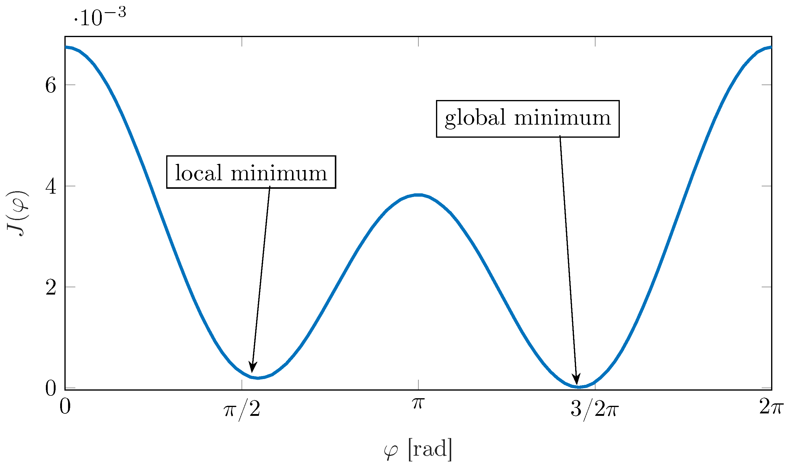
When nonlinear constraints are included, finding the optimal voltage vector to apply in the next control step is problematic, since it involves finding the minimum multivariable function, and the computational effort can be very high [27]. The applicability of the continuous-set predictive control algorithm on low-cost applications, such as electric pumps, is therefore undermined by the need for expensive microprocessors.

In order to reduce the computational complexity of continuous-set predictive control, the present paper proposes a simplification of the minimisation problem based on setting a maximum voltage vector amplitude, so that the search will be conducted on the phase of the voltage vector only. The low complexity search algorithm was combined with a model-free technique that predicts the currents variations by means of an efficient RLS algorithm [25]. The result is a very practical current control solution that can be implemented on any industrial drive for pump applications.

In order to demonstrate the feasibility of the proposed technique, a test case was provided and analysed, including two different industrial inverter-driven SynRMs. Both the inverter and motors are supposed to be powered by a conventional 400 $\mathrm{V}$ three-phase grid supply. However, the test case provided in this paper will simulate the case where only a 230 $\mathrm{V}$ single-phase grid supply is available, which is realistic for many developing countries where the three-phase grid is not widespread. Each test motor has been connected to the inverter without any initial calibration, to prove the generality of the proposed control algorithm.

This paper is structured as follows. The model-free current variations prediction and the RLS algorithm implementations are discussed in Section 2. The core of this paper is the new predictive control algorithm reported in Section 3, where the new optimisation problem formulation and the computational cost-effective algorithm for finding the optimum voltage vectors are described. The experimental results are reported in Section 4, and are followed by thorough discussions and considerations. Final conclusive remarks are reported in the Conclusion in Section 5.

2. Mathematical Background

The motor voltage balance equations are written in the dq reference frame, synchronously with the rotor. The d axis position in a SynRM corresponds to the position where the reluctance value is minimum, and its angular displacement is defined as ${\vartheta }_{\mathrm{me}}$. The $dq$ voltage balance equations are:

$${\mathbf{u}}_{dq}=R{\mathbf{i}}_{dq}+\left[\begin{array}{cc}{l}_d(i_d,i_q)& 0\\ 0& l_q(i_d,i_q)\end{array}\right]{\displaystyle \frac{d{\mathbf{i}}_{dq}}{dt}}+{\omega }_{\mathrm{me}}\left[\begin{array}{cc}0& -1\\ 1& 0\end{array}\right]{\lambda }_{dq}(i_d,i_q)$$

(1)

where ${\mathbf{u}}_{dq}={[u_d,u_q]}^T$ and ${\mathbf{i}}_{dq}={[i_d,i_q]}^T$ are the voltage and current vectors, respectively, R is the stator resistance, $l_d\triangleq \partial {\lambda }_d(i_d,i_q)/\partial i_d$ and $l_q\triangleq \partial {\lambda }_q(i_d,i_q)/\partial i_q$ are the d and q axis differential inductances, ${\lambda }_{dq}={[{\lambda }_d(i_q,i_q),{\lambda }_q(i_q,i_q)]}^T$ is the magnetic flux linkages vector and ${\omega }_{\mathrm{me}}$ is the electrical speed. The current dependence $(i_d,i_q)$ in the differential inductances and magnetic flux linkages is omitted in the following for the sake of brevity. The symbol ≜ stands for definition.

To ease the mathematical expression, only the d axis voltage balance equation is considered at first. Actually, the q axis voltage balance equation presents the same equation structure; thus, the same analytical results are obtained. The current dynamics can be derived from (1) as

$$\begin{array}{c}\hfill \frac{d{i}_d}{dt}=-\frac{R{i}_d+{\lambda }_q{\omega }_{\mathrm{me}}}{l_d}+\frac{u_d}{l_d}.\end{array}$$

(2)

Observing Equation (2) and considering the discrete nature of the control system, the current variation at each control period $T_c$ can be expressed by the following new adaptive model:

$$i_d\left(k\right)-i_d(k-1)\triangleq \Delta i_d\left(k\right)=p_{1,d}\left(k\right)+p_{2,d}\left(k\right)u_d\left(k\right)$$

(3)

where $p_{1,d}\left(k\right)$ and $p_{2,d}\left(k\right)$ are coefficients that are adapted during online operations. The adaptation strategy is crucial for the correct estimation of the current variations predictions. A recursive least square algorithm was adopted in this work for the adaptation of the coefficients based on previous current measurements and applied voltage vectors as in [25].

Adaptive Model by Recursive Least Square Algorithm

For the sake of generality, both currents variations can be rearranged as follows:

$$\begin{array}{cc}\hfill \Delta i_d\left(k\right)& =\left[1,u_d\left(k\right)\right]{\left[p_{1,d},p_{2,d}\right]}^T={\mathit{\varphi }}_d\left(k\right){\mathbf{p}}_d\left(k\right)\hfill \\ \hfill \Delta i_q\left(k\right)& =\left[1,u_q\left(k\right)\right]{\left[p_{1,q},p_{2,q}\right]}^T={\mathit{\varphi }}_q\left(k\right){\mathbf{p}}_q\left(k\right)\hfill \end{array}$$

(4)

where ${\mathit{\varphi }}_d$ and ${\mathit{\varphi }}_q$ are the regressors’ vectors, ${\mathbf{p}}_d$ and ${\mathbf{p}}_q$ are the adaptive coefficients vectors of the d and q axes, respectively. The standard RLS algorithm, as can be seen in [28], can be recursively solved by the following set of equations:

$$\begin{array}{cc}\hfill \mathbf{G}\left(k\right)& =\mathbf{Q}(k-1){\mathsf{\Phi }}^T\left(k\right){\left(\mathsf{\Phi }\left(k\right)\mathbf{Q}(k-1){\mathsf{\Phi }}^T\left(k\right)+f\mathbf{I}\right)}^{-1}\hfill \\ \hfill \widehat{\mathbf{p}}\left(k\right)& =\widehat{\mathbf{p}}(k-1)+\mathbf{G}\left(k\right)\left(\mathbf{y}\left(k\right)-\mathsf{\Phi }\left(k\right)\widehat{\mathbf{p}}(k-1)\right)\hfill \\ \hfill \mathbf{Q}\left(k\right)& =f^{-1}\left(\mathbf{Q}(k-1)-\mathbf{G}\left(k\right)\mathsf{\Phi }\left(k\right)\mathbf{Q}(k-1)\right)\hfill \end{array}$$

(5)

where $\mathbf{G}\left(k\right)\in {\mathbb{R}}^{4\times 4}$ is the gain matrix, $\mathbf{Q}\left(k\right)\in {\mathbb{R}}^{4\times 4}$ is the estimated error covariance matrix, $\mathsf{\Phi }\left(k\right)\in {\mathbb{R}}^{4\times 4}$ is the regressors’ matrix, f is the scalar forgetting factor, $\widehat{\mathbf{p}}\triangleq {[{\widehat{\mathbf{p}}}_d,{\widehat{\mathbf{p}}}_q]}^T$ is the ${\mathbb{R}}^{4\times 1}$ coefficients vector and $\mathbf{y}\in {\mathbb{R}}^{4\times 1}$ is the measurements vector.

In order to estimate four parameters, at least four linearly independent and uncorrelated measurements are necessary. However, only two measurements are available during the current control period k, i.e., one for each of the $dq$ axes. The additional two measurements can be retrieved by using the current measurements during the previous control period $(k-1)$. Therefore, the vector of measurements is defined as follows:

$$\mathbf{y}\left(k\right)={[\Delta i_d\left(k\right),\Delta i_d(k-1),\Delta i_q\left(k\right),\Delta i_q(k-1)]}^T$$

(6)

The regressors’ vector $\mathsf{\Phi }$ can be written in the same fashion of (6) by adopting the voltage measurements of the actual $\left(k\right)$ and previous $(k-1)$ control periods.

The future currents can be predicted based on the assumption that the coefficients $\widehat{\mathbf{p}}$ are constant for at least two discrete sampling time periods $T_c$. As an example, the d axis current evolution can be estimated as follows:

$$\begin{array}{cc}\hfill {\widehat{i}}_d(k+1)& =i_d\left(k\right)+{\widehat{p}}_{1,d}\left(k\right)+{\widehat{p}}_{2,d}\left(k\right)·u_d\left(k\right)\hfill \\ \hfill {\widehat{i}}_d(k+2)& ={\widehat{i}}_d(k+1)+{\widehat{p}}_{1,d}\left(k\right)+{\widehat{p}}_{2,d}\left(k\right)·u_d(k+1)\hfill \end{array}$$

(7)

More details about the current predictions based on the adaptive model by recursive least squares algorithm, such as the tuning of the forgetting factor parameter f, are available in [25]. It is worth highlighting that the voltage $u_d(k+1)$ is an unknown value as well as $u_q(k+1)$. These two voltage values are the voltages that shall be applied at time instant $k+1$. An optimisation algorithm is thus developed in Section 3 to determine the optimal voltage reference vector ${\mathbf{u}}_{dq}^{*}(k+1)={[u_d^{*}(k+1),u_q^{*}(k+1)]}^T$ at every control time $T_c$.

3. Proposed Deadbeat Predictive Current Control

In order to determine the voltage reference vector ${\mathbf{u}}_{dq}^{*}(k+1)$, the quadratic cost function adopted in this paper is:

$$J={∥{\mathbf{i}}_{dq}^{*}\left(k\right)-{\widehat{\mathbf{i}}}_{dq}(k+2)∥}^2$$

(8)

where only the current error must be minimised and the current vector prediction ${\widehat{\mathbf{i}}}_{dq}(k+2)$ is calculated as in (7). Evaluating a quadratic cost function instead of a simpler absolute tracking error can significantly improve its performance and prevent the stability issue as mentioned in [29]. A two-variable minimisation problem is required by (8) due to the reference voltage vector ${\mathbf{u}}_{dq}^{*}(k+1)$, which is a $2\times 1$ vector. In order to always provide feasible solutions, a constrained minimisation problem should also be adopted. Therefore, the computational burden required by the two-variable minimisation constrained problem algorithm would be cumbersome to handle by reduced computational power microprocessors.

3.1. Proposed Choice of Voltage Vector Module and Design Hints

In this paper, a simplified approach for the minimisation of (8) was adopted by introducing a constraint on the voltage vector magnitude. The voltage reference vector can be rewritten in polar coordinates as ${\mathbf{u}}_{dq}^{*}(k+1)=U(k+1)e^{j\phi (k+1)}$, where U and $\phi$ are the voltage reference vector magnitude and phase, respectively, in the synchronous reference frame. The superscript ${}^{*}$, which means a reference quantity, in $U(k+1)$ and $\phi (k+1)$, was omitted for simplicity. The magnitude U was assumed to be constant within one control period and its value was set before the optimisation algorithm was executed. It turned out that the requirement of obtaining a feasible solution was automatically satisfied, provided that the voltage magnitude U is chosen within the feasible set $u_{\mathrm{bus}}/\sqrt{3}$, where $u_{\mathrm{bus}}$ is the inverter bus voltage. The feasible set graphical representation is reported in Figure 1. The choice of a continuous set of values for ${\mathbf{u}}_{dq}^{*}(k+1)$ requires the use of a pulse width modulator (PWM), which is an additional computational burden with respect to a finite-set solution. Actually, PWM algorithms are very widespread and optimised since they are even necessary in conventional linear controllers. For instance, the space vector modulation algorithm is very popular and efficient from a computational point of view.

The quantity $U(k+1)$ can be set as subject to different design requirements. The first trivial solution is to choose an always constant value, i.e., $U=U_{\max }\triangleq u_{\mathrm{bus}}/\sqrt{3}$. However, the advantages of using a voltage modulator would be wasted. When a small voltage magnitude is required, e.g., at low speed, the choice $U=U_{\max }$ forces the solution of (8) to be larger than necessary. The consequence is a large current ripple making this first trivial choice equivalent to a finite-set solution. Following the model-free paradigm that no motor parameters should be used to design the current control algorithm, the choice of $U(k+1)$ should be made, balancing both the advantage of having a voltage modulator and the simplicity of implementation.

As a design hint, the variation law of $U(k+1)$ can be selected similarly to the $\mathrm{V}$/$\mathrm{Hz}$ control strategy often adopted in induction motor drives. The simple consideration that the voltage magnitude is strongly proportional to the motor speed can be used to set the desired variation law of $U(k+1)$. Bearing in mind that the voltage magnitude value is set as constant during one control period in the cost function (8), a lower case variable is introduced to represent the variable magnitude of the voltage reference vector, i.e., $u(k+1)$. Furthermore, the speed dependence of $u(k+1)$ was highlighted by dropping the $(k+1)$ time notation and rewriting the voltage magnitude value as a function of the speed, i.e., $u\left({\omega }_{\mathrm{m}}\right)$. Actually, the experimental activity carried out in Section 4 has shown a technically sound solution, which is represented by using the speed reference quantity, thus obtaining $u\left({\omega }_{\mathrm{m}}^{*}\right)$.

The final variation law of $u\left({\omega }_{\mathrm{m}}^{*}\right)$ adopted in this paper is:

$$u\left({\omega }_{\mathrm{m}}^{*}\right)=u_{\min }+k_{\omega }·{\omega }_{\mathrm{m}}^{*}$$

(9)

where $k_{\omega }=(u_{\max }-u_{\min })/{\omega }_n$. A second design hint is concerned with the selection of the minimum value $u_{\min }$ for the voltage module $u\left({\omega }_{\mathrm{m}}^{*}\right)$. The simplest meaning of $u_{\min }$ is that a minimum amount of voltage is necessary at zero speed to balance the resistance voltage drop and obtain the nominal current value. During transient operations, the derivative terms of (1) are not zero—even at null speed. Therefore, additional voltage to the resistance voltage drop is necessary to obtain fast current transients. A choice was made to set $u_{\min }=40\%u_{\max }$. The effects of the different $u_{\min }$ values choice is discussed in Section 4.4.

3.2. Proposed Optimisation Problem

The only variable that can be used to minimise the cost function (8) is the voltage reference vector phase $\phi (k+1)$. The cost function (8) can be rewritten with the aid of (7) as follows:

$$J\left(\phi (k+1)\right)={\left[{\delta }_d-{\widehat{p}}_{2,d}u\left({\omega }_{\mathrm{m}}^{*}\right)cos\left(\phi (k+1)\right)\right]}^2+{\left[{\delta }_q-{\widehat{p}}_{2,q}u\left({\omega }_{\mathrm{m}}^{*}\right)sin\left(\phi (k+1)\right)\right]}^2$$

(10)

where ${\delta }_d\left(k\right)\triangleq i_d^{*}\left(k\right)-{\widehat{i}}_d(k+1)-p_{1,d}$ and ${\delta }_q\triangleq i_q^{*}\left(k\right)-{\widehat{i}}_q(k+1)-p_{1,q}$. It is worth recalling the polar representation of the voltage reference vector:

$$\begin{array}{cc}\hfill u_d(k+1)& =u\left({\omega }_{\mathrm{m}}^{*}\right)cos\left(\phi (k+1)\right)\hfill \\ \hfill u_q(k+1)& =u\left({\omega }_{\mathrm{m}}^{*}\right)sin\left(\phi (k+1)\right)\hfill \end{array}$$

(11)

The feasible region where the voltage reference vector lies is sketched in Figure 1 and is highlighted in green colour. The dotted blue circumference reported in Figure 1 represents an example of a solution locus set for a given reference speed ${\omega }_{\mathrm{m}}^{*}$. It is worth remarking that no constraints are needed for solving the optimisation problem (10) since $u_{max}\le u_{\mathrm{bus}}/\sqrt{3}$ always guarantees feasible solutions.

3.3. Algorithm for Finding the Optimal Solution

The minimisation problem with the cost function (10) requires a non-linear single variable solver. Several efficient algorithms can be adopted. The golden section search (GSS) algorithm was adopted in this paper due to its simplicity and computational efficiency [30]. The solution of problem minimisation during each control period is given by

$$\phi (k+1)=\mathbf{GSS}\left(J\left(\phi \right(k+1\left)\right),\mathrm{lb},\mathrm{ub},ϵ,\mathrm{iter}\right)$$

(12)

where the required input arguments are:

• $J\left(\phi \right(k+1\left)\right)$: the function that has to be minimised (i.e., Equation (10));
• lb: lower bound of the searching interval;
• ub: upper bound of the searching interval;
• $ϵ$: termination tolerance for searching the solution;
• iter: maximum number of algorithm iterations for finding the solution.

An important aspect that must be taken into account is the non-monotonic behaviour of the cost function. The presence of trigonometric terms $cos\left(x\right)$ and $sin\left(x\right)$ results in more than one minimum over the $\left[0,2\pi \right]$ domain. Further investigations about the cost function (10) reveal that only one minimum occurs in either one of the sub-sets $\left[0,\pi \right]$ and $\left[\pi ,2\pi \right]$. An example of the cost function behaviour is reported in Figure 2. In order to avoid the convergence of the algorithm to a local minimum instead of a global one, the search interval was split in two: the first interval was set as $\left[0,\pi \right]$; and the second one as $\left[\pi ,2\pi \right]$. The minimisation algorithm (12) was executed twice—one for each searching interval. The two $\phi (k+1)$ solutions were than compared, and the one returning the lowest total cost value was selected.

An important aspect regarding the implementation of model predictive control is the computational burden required by the minimisation algorithm. The two parameters that affect the computational requirement of the algorithm in (12) are the termination tolerance $ϵ$ and the maximum number of algorithm iterations iter. The former parameter is related to the accuracy of the calculated voltage phase $\phi (k+1)$. In other words, the termination tolerance is related to the difference between two iterative solutions of the algorithm (12). When the difference is below the termination tolerance, the algorithm has found the minimum of the function. Therefore, a technically sound value of $ϵ$ is $0.01$ rad, i.e., approximately 0.5. The latter parameter iter allows to estimate the worst case conditions in terms of computational time consumption, thus preventing overrun conditions that are extremely dangerous for real-time applications. The value of iter depends on the microprocessor adopted in the electrical drive. A possible solution is to estimate the computational time required by running the algorithm (12) one time and determining the maximum number of iterations possible on the available hardware. Finally, it is worth pointing out that both $ϵ$ and iter do not depend on the motor under test but only on the computational hardware, in accordance with the model-free paradigm proposed in this paper.

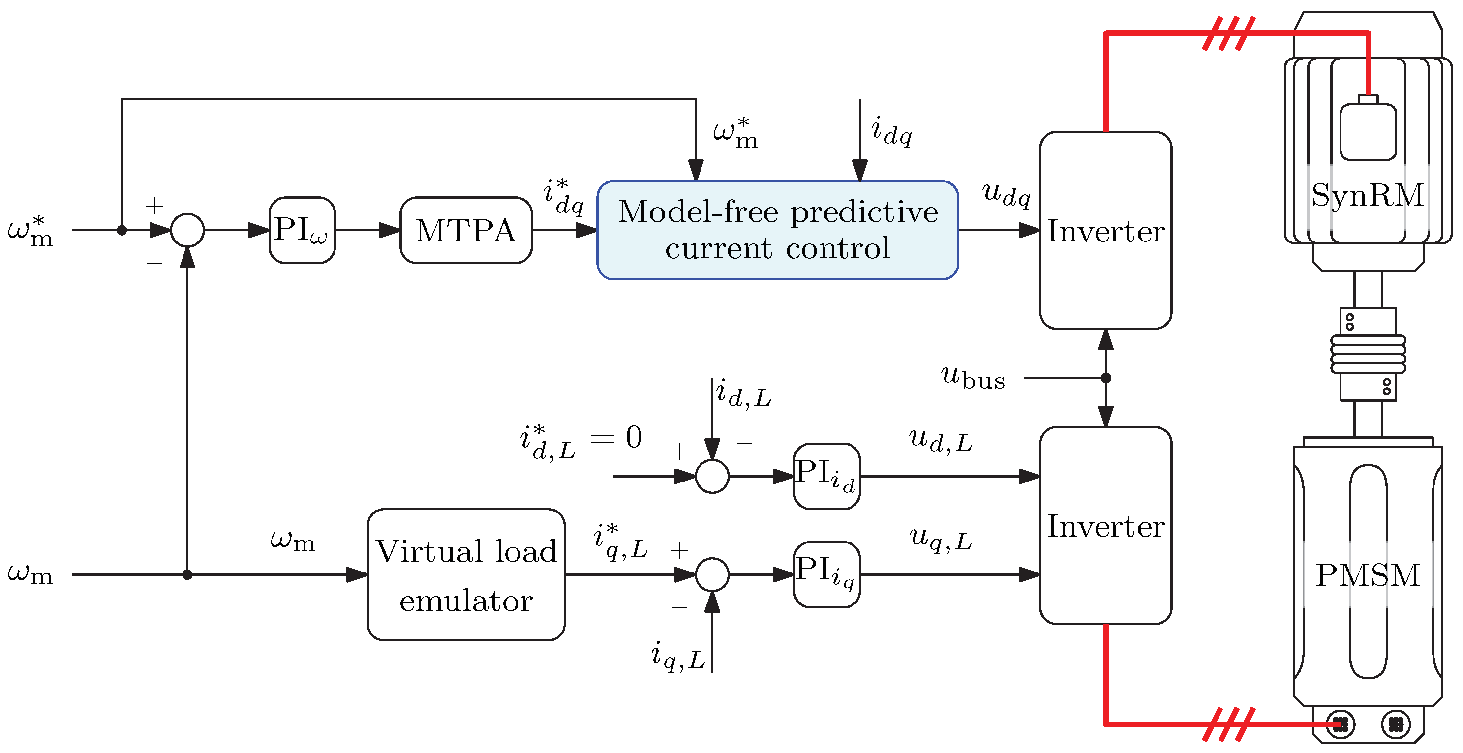
4. Experimental Results and Discussion

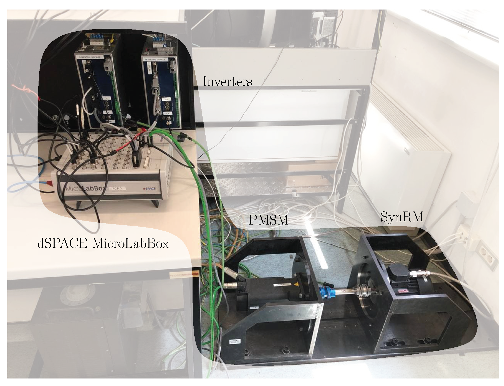
The control algorithm reported in Section 3 was implemented on a fast control prototyping test rig (Figure 3) dSpace MicroLabBox featuring a SynRM acting as a motor under test and an isotropic permanent magnet synchronous motor (PMSM) acting as a virtual load. The sampling and switching frequency were both set to 8 $\mathrm{k}$$\mathrm{Hz}$. It is worth highlighting that a higher switching frequency introduces only benefits in terms of current ripple, but at the price of additional switching losses and a reduced equivalent time for the control algorithm to be carried out.

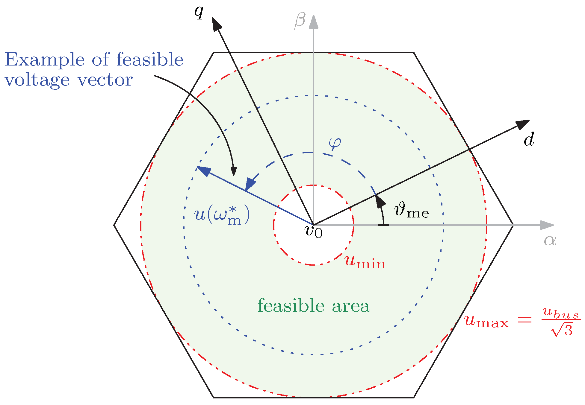
In order to represent a realistic scenario, the bus voltage was set considering a single-phase 230 $\mathrm{V}$ grid supply. However, the two motors under test of

Table 1. Motors under test nameplate parameters.

Parameter	Symbol	Unit	SynRM${}_1$	SynRM${}_2$
Resistance	R	$\mathrm{\Omega }$	$4.6$	$1.8$
d axis inductance (unsat.)	$L_d$	$\mathrm{m}\mathrm{H}$	380	340
q axis inductance (unsat.)	$L_q$	$\mathrm{m}\mathrm{H}$	85	60
Nominal current	$I_n$	$\mathrm{A}$	4	$5.6$
Nominal speed	${\mathrm{\Omega }}_n$	$\mathrm{rpm}$	1500	1500
Nominal power	$P_n$	$\mathrm{W}$	1600	2200
Nominal torque	${\tau }_n$	$\mathrm{N}\mathrm{m}$	$10.2$	$14.0$

considered in this work were designed for three-phase grid supplied inverters. The situation could take place in those geographical areas where the three-phase grid supply is not available. The solar pumps represent another example where the bus voltage is lower than in the industrial case, but the available motors windings are designed for the full bus voltage value. The schematic of the proposed experimental setup is sketched in Figure 4. Simple PI speed control was implemented and a traditional 45 MTPA strategy [31] was adopted since the main focus was the current control and not the current references generation.

The only parameters that must be chosen in the proposed current control algorithm are the forgetting factor f in (5) and $u_{\min }$ in (9). The former parameter, f, can be set to a constant value equal to $0.99$ with little reflections on the current dynamic performance deterioration, as can be seen in [25]. The minimum voltage $u_{\min }$ is set to $25\%$ of $u_{\max }$, which is a fair approximation that guarantees the balance of the Joule losses at all working points. It is worth pointing out that the $u_{\min }$ value could be set to lower (or higher) values provided that the motor resistance is known. However, the $u_{\min }$ value slightly affects the dynamic of the currents, but the current tracking is guaranteed.

4.1. Design of Experiment: The Pump Load Emulator

The behaviour of an electric pump was emulated by means of a PMSM drive coupled to the motor under test and programmed as a virtual load. This is a very practical and common approach, which can be extended to represent many different loads behaviours, e.g., [32].

The load torque ${\tau }_L$ characteristic of a pump can be approximated by the sum of two terms. The first contribution is the friction torque ${\tau }_F$, which includes a constant term due to dry friction $B_{0,F}$ and a term proportional to the speed due to motor ventilation. The second contribution is the pump torque ${\tau }_P$, which depends on the pump type under consideration. A centrifugal pump was considered in this paper, and the total load torque ${\tau }_L$ was calculated as follows:

$$\begin{array}{cc}\hfill {\tau }_F& =B_1{\omega }_m+B_{0,F}\hfill \\ \hfill {\tau }_P& =B_2{\omega }_m^2\hfill \\ \hfill {\tau }_L& ={\tau }_F+{\tau }_P=B_2{\omega }_m^2+B_1{\omega }_m+B_0\hfill \end{array}$$

(13)

where $B_0=B_{0,F}$ for the sake of brevity. The values of the parameters $B_0$, $B_1$ and $B_2$ were decided in order to guarantee that the nominal torque was produced by the motor under test when operating at nominal speed. Bearing in mind that the nominal speed values were reduced to meet the voltage constraint requirement set by the limited bus voltage, the values of the parameters adopted during the experimental stage are reported in

Table 2. Parameters of the virtual load emulator in (13).

Parameter	SynRM${}_1$	SynRM${}_2$
Static friction $B_0$	$0.5542$	$0.5542$
Ventilation friction $B_1$	$9.1\times {10}^{-3}$	$9.1\times {10}^{-3}$
Pump friction $B_2$	$7.77\times {10}^{-4}$	$11.65\times {10}^{-4}$

.

In order to evaluate the current control algorithm proposed in this paper, a simple test was designed.

The motor under test was set in speed control mode, while the load motor was torque controlled as sketched in Figure 4. The desired load torque ${\tau }_L$ (13) was guaranteed by applying the following current references:

$$\begin{array}{cc}\hfill i_{d,L}^{*}& =0\hfill \end{array}$$

(14)

$$\begin{array}{cc}\hfill i_{q,L}^{*}& ={\displaystyle \frac{2}{3}}{\displaystyle \frac{{\tau }_L}{p{\lambda }_{mg,L}}}\hfill \end{array}$$

(15)

where ${\lambda }_{mg,L}$ is the load permanent magnet flux, and p is the load pole pairs. The subscript L denotes (also in Figure 4) load quantities.

4.2. Pump Load Emulator Results

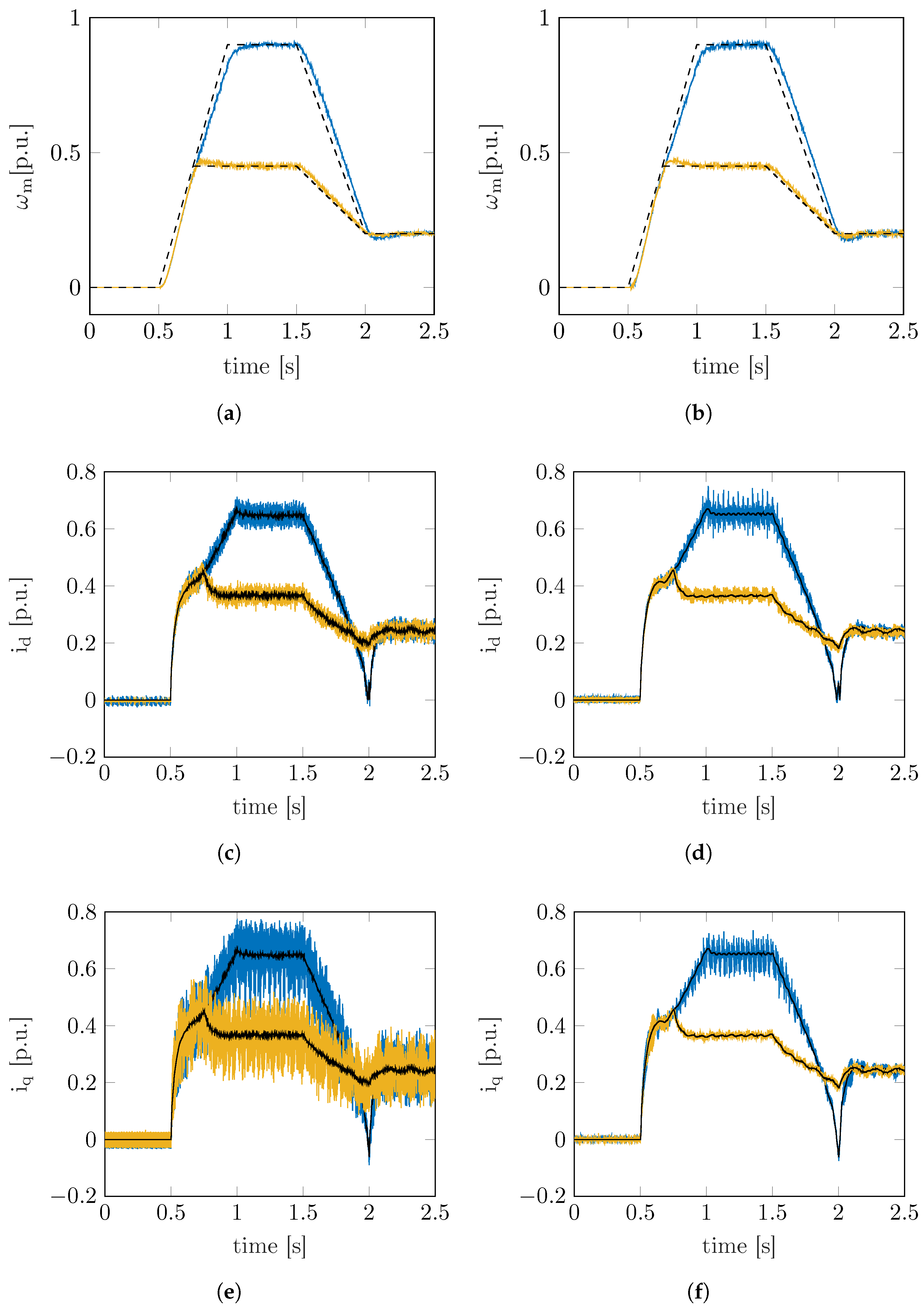
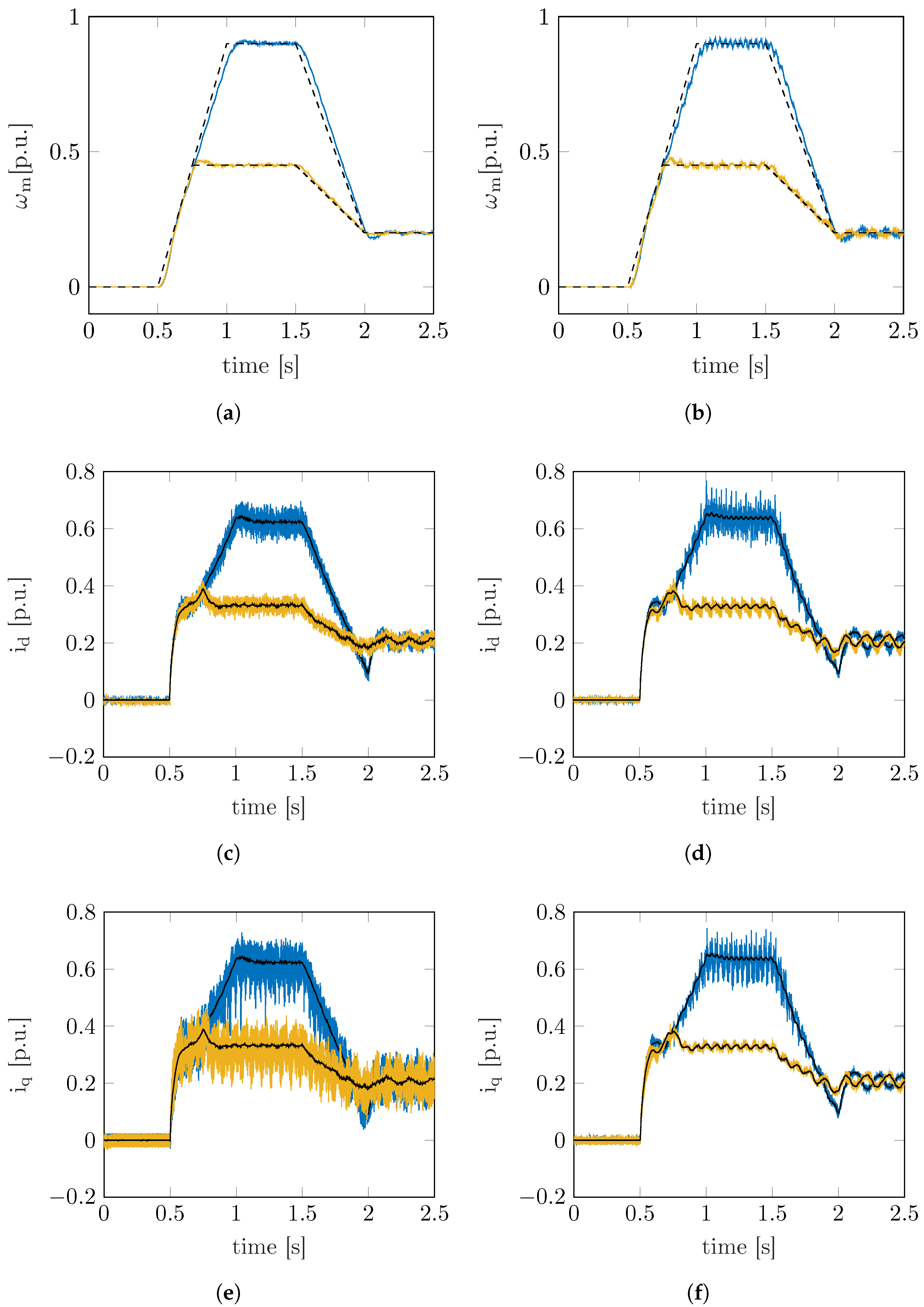
Two different speed set points were evaluated. The speed and current measurements as well as the references of the two motors under test are reported in Figure 5 and Figure 6. The comparison with the benchmark model-free finite-set predictive current control proposed in [25] is also reported. The characteristic pump toque load behaviour is evident during the acceleration phase in both $dq$ axes currents, which show a parabolic curve-like characteristic in Figure 5c–f for the SynRM${}_1$ motor under test. The same applies for the current measurements of the SynRM${}_2$ motor under test reported in Figure 6.

The current ripple is considerably reduced for both motors under test by using the proposed model-free predictive current control. This was obtained since the equivalent voltage vector obtained by the predictive control proposed in Section 3 was selected in a continuous-set domain rather than a finite-set domain as in [25]. The equivalent switching frequency of the finite-set predictive current controller is surely lower than that of the proposed control, which is fixed at 8 $\mathrm{k}$$\mathrm{Hz}$. Finite-set algorithms are known for their unpredictable switching frequency, which depends on the optimal voltage vector sequence applied during runtime operation. From the current ripple reduction point of view in the finite-set algorithm, the higher the control frequency, the better. However, the control time period is of utmost importance when the computational capacity of the microcontroller is under consideration.

The computational burden required by the proposed method remains limited. The benchmark finite-set algorithm requires an average turnaround time of the microcontroller routine of 34 $\mu$$\mathrm{s}$, i.e., the $27.2\%$ of the control period $T_c$. The proposed model-free predictive current control required an average turnaround time of 42 $\mu$$\mathrm{s}$, i.e., the $33.6\%$ of $T_c$. In other words, the proposed model-free predictive current control algorithm requires $6.4\%$ of $T_c$ more than the benchmark finite-set method.

It is worth remarking that no parameter tuning was required in the proposed current control algorithm of Section 3 for both motors under test. This is a distinctive feature of the proposed model-free predictive control algorithm which can be applied to different SynRMs without the need for any knowledge of motor parameters’ values. Furthermore, the algorithm proposed in Section 3 can also be applied to permanent magnet motors, provided that the current ripple value remains limited.

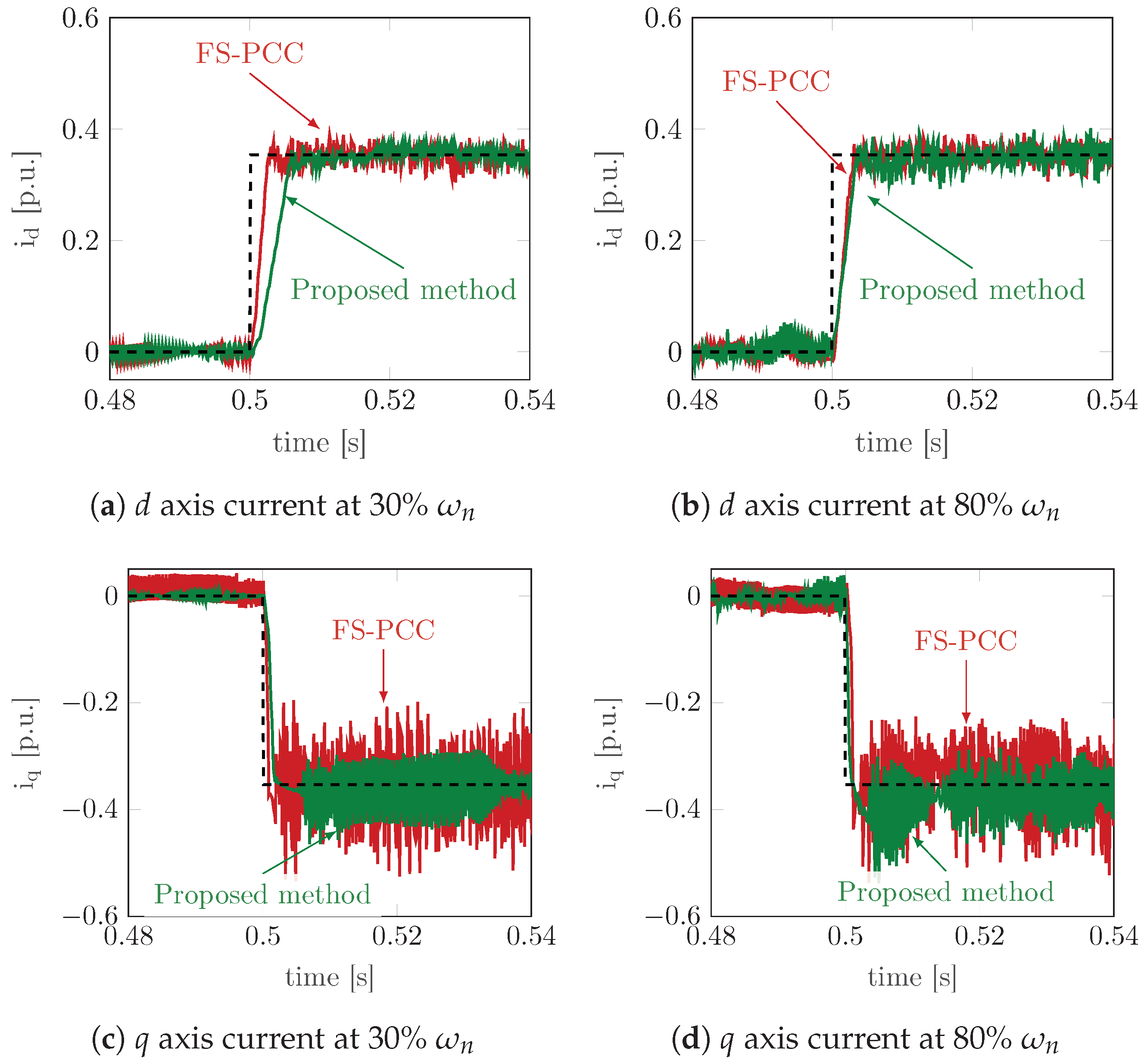
4.3. Load Step Variations

In order to test the current reference tracking capability of the proposed model-free predictive current control, a further test was carried out. A current step reference variation situation is likely to occur in a pump application when a denser fluid suddenly hits the pump. Nonetheless, the test is a canonical procedure to verify the capability of the control algorithm under consideration and thus, general considerations can be drawn.

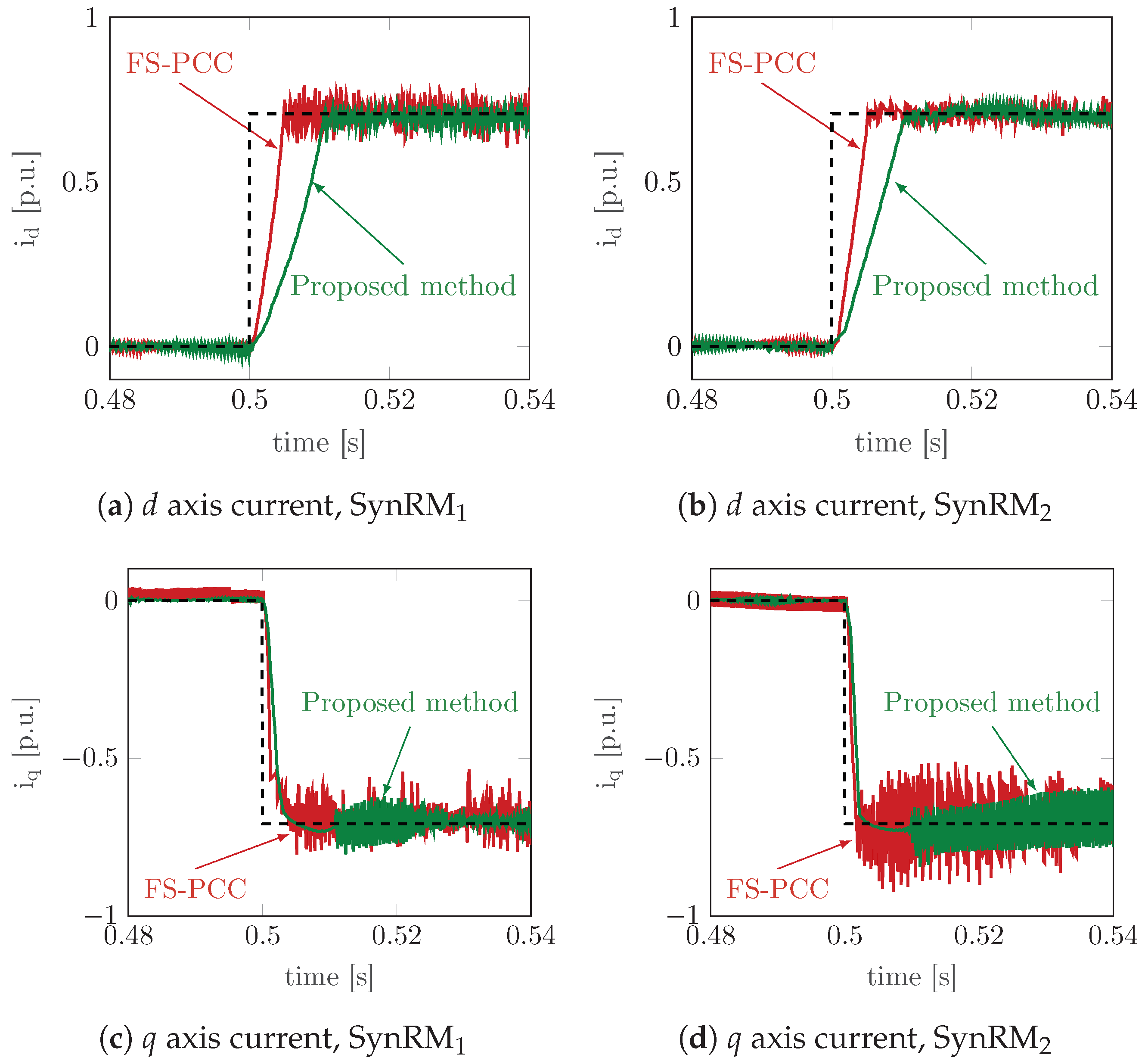
The motor under test was dragged by the virtual load motor at constant speed, namely $30\%$ of the motor under test nominal speed, while only the current control was active. A current magnitude reference equal to half the nominal value was imposed, and the results were reported in Figure 7 for both motors under test.

On the one hand, the q axis current dynamics obtained by the proposed model-free predictive control was almost the same as for the benchmark finite-set predictive control, as can be seen in Figure 7c,d. The steady state behaviour shows that the proposed model-free control algorithm yields a smaller current ripple than the benchmark finite-set predictive controller. The results confirm the steady state behaviour of the q axis current measurements obtained in the pump tests of Section 4.2, in particular Figure 5e compared to Figure 5f and Figure 6e compared to Figure 6f.

On the other hand, the d axis current dynamics reported in Figure 7a,b shows that the benchmark finite-set controller is faster than the proposed one. The reason is the smaller available voltage of the proposed model-free controller compared to the finite-set one of [25], since the voltage is limited by the $u\left({\omega }_{\mathrm{m}}^{*}\right)$ law in (9). The effect is preponderant on the d axis tracking performances due to the larger value of $L_d$ compared to $L_q$ in SynRMs. This is the major drawback of the proposed model-free predictive control which is counterbalanced by a better steady state behaviour compared to the finite-set predictive control. It is worth highlighting that the proposed model-free predictive control is designed for pump applications, who are unlikely to require very high dynamic performances from the current controller.

A second batch of measurements with step-like variation of the current reference was collected with the SynRM${}_2$ as the motor under test, aiming to testing the proposed current control performances at different load and speed values. The results of the second batch are reported in Figure 8. The current dynamics of both $dq$ axes currents in Figure 8a,c are very similar to the ones at the rated current in Figure 7b,d, respectively, which is at low speed. However, the current tracking dynamics at higher speed is sensibly improved by the proposed d axis current predictive controller, as reported in Figure 8b. The reason is that a higher voltage value $u\left({\omega }_{\mathrm{m}}^{*}\right)$ is available for the minimisation of the cost function (10), since the reference speed is higher in (9). It is worth recalling that the load torque value in pump applications increases with the speed. Therefore, improvement of current tracking performances with the increase in the speed of the proposed model-free predictive control is attractive for pump applications.

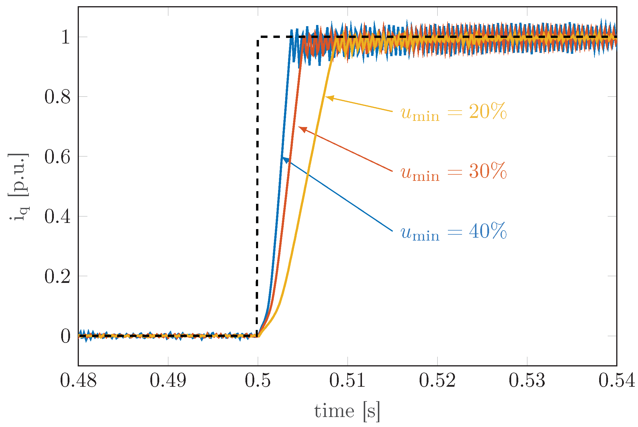
4.4. Effects of Different $u_{\min }$ Values

The $u_{\min }$ value is the only parameter of the proposed current control that apparently requires tuning. Three different d axis current measurements using different $u_{\min }$ values and imposing a rated current step variation at null speed are reported in Figure 9. The current dynamics during the transient is penalised as the $u_{\min }$ value decays; however, the current ripple amplitude also decreases, which improves the steady state behaviour of the current controller.

A conservative choice for the $u_{\min }$ value was made following the model-free control paradigm. The 25 % of $u_{\max }$ is a reasonable choice because it provides good current dynamics and simultaneously improves the current ripple compared to the finite-set algorithm, as can be seen in Figure 5 and Figure 6. It is worth pointing out that the purpose of this paper was to propose a proof of concept about a new continuous-set model-free predictive control and highlight the implementation aspects that determine the functioning of the algorithm. The $u_{\min }$ value can be set by different simple strategies that do not involve specialised human interaction, such as the choice between two predetermined values.

5. Conclusions

A new continuous-set model-free predictive current control was studied in this paper, addressing simple, low-cost electric pump applications.

As a distinguishing feature, the proposed predictive control was based on an adaptive RLS-based model, which is linked to but not constrained by knowledge of any specific motor parameter. This fact, combined with a simplified search strategy within a continuous set of voltage vectors, resulted in efficient, low-cost, and low-ripple current control. The proposed current control skips any initial motor calibration, allowing an immediate operational startup with a generic electric pump based on the SynRM. In addition to this, there are many other applications where this control can be applied with higher benefits if compared with the traditional linear controller.

The validity of the proposed control was proven by several tests on an experimental test rig featuring two different SynRMs and the results were thoroughly discussed.

Simple and automatic initial self-tuning has the invaluable advantage of not requiring the presence of expert personnel either at the first start-up or in case of the replacement of a faulty motor.

In conclusion, the proposed strategy makes use of complex technology to achieve similar or better results than PI control and finite set model-free predictive control with the specific goal of making the complexity transparent to the end user, as an established trend in any smart home device.

References

1. Pellegrino, G.; Jahns, T.; Bianchi, N.; Soong, W.; Cupertino, F. The Rediscovery of Synchronous Reluctance and Ferrite Permanent Magnet Motors; Springer International Publishing: Berlin/Heidelberg, Germany, 2016. [Google Scholar] [CrossRef]
2. Angadi, S.; Yaragatti, U.R.; Suresh, Y.; Raju, A.B. Comprehensive review on solar, wind and hybrid wind-PV water pumping systems-an electrical engineering perspective. CPSS Trans. Power Electron. Appl. 2021, 6, 1–19. [Google Scholar] [CrossRef]
3. Farhan, A.; Abdelrahem, M.; Hackl, C.M.; Kennel, R.; Shaltout, A.; Saleh, A. Advanced Strategy of Speed Predictive Control for Nonlinear Synchronous Reluctance Motors. Machines 2020, 8, 44. [Google Scholar] [CrossRef]
4. Van Rhyn, P.; Pretorius, J.H.C. Increasing Water Pump Station Throughput by Introducing VFD-Based IE4 Class Synchronous Reluctance Motors with Improved Pump Control. In Proceedings of the 2018 IEEE International Conference on Environment and Electrical Engineering and 2018 IEEE Industrial and Commercial Power Systems Europe (EEEIC/I CPS Europe), Palermo, Italy, 12–15 June 2018; pp. 1–6. [Google Scholar] [CrossRef]
5. Oliveira, F.; Ukil, A. Comparative Performance Analysis of Induction and Synchronous Reluctance Motors in Chiller Systems for Energy Efficient Buildings. IEEE Trans. Ind. Inform. 2019, 15, 4384–4393. [Google Scholar] [CrossRef]
6. Ibrahim, M.N.; Rezk, H.; Al-Dahifallah, M.; Sergeant, P. Hybrid Photovoltaic-Thermoelectric Generator Powered Synchronous Reluctance Motor for Pumping Applications. IEEE Access 2019, 7, 146979–146988. [Google Scholar] [CrossRef]
7. Ibrahim, M.N.; Rezk, H.; Al-Dhaifallah, M.; Sergeant, P. Solar Array Fed Synchronous Reluctance Motor Driven Water Pump: An Improved Performance Under Partial Shading Conditions. IEEE Access 2019, 7, 77100–77115. [Google Scholar] [CrossRef]
8. Pasqualotto, D.; Tinazzi, F.; Zigliotto, M. Enhanced solar water-pumping system driven by a synchronous reluctance motor. In Proceedings of the 2021 22nd IEEE International Conference on Industrial Technology (ICIT), Valencia, Spain, 10–12 March 2021; Volume 1, pp. 365–370. [Google Scholar] [CrossRef]
9. Varshney, A.; Sharma, U.; Singh, B. An Intelligent Grid Integrated Solar PV Array Fed RSM Drive-Based Water Pumping System. IEEE Trans. Ind. Appl. 2021, 57, 1818–1829. [Google Scholar] [CrossRef]
10. Antonello, R.; Ortombina, L.; Tinazzi, F.; Zigliotto, M. Advanced current control of synchronous reluctance motors. In Proceedings of the 2017 IEEE 12th International Conference on Power Electronics and Drive Systems (PEDS), Honolulu, HI, USA, 12–15 December 2017; pp. 1037–1042. [Google Scholar] [CrossRef]
11. Ortombina, L.; Pasqualotto, D.; Tinazzi, F.; Zigliotto, M. Magnetic Model Identification of Synchronous Motors Considering Speed and Load Transients. IEEE Trans. Ind. Appl. 2020, 56, 4945–4954. [Google Scholar] [CrossRef]
12. Hinkkanen, M.; Pescetto, P.; Mölsä, E.; Saarakkala, S.E.; Pellegrino, G.; Bojoi, R. Sensorless Self-Commissioning of Synchronous Reluctance Motors at Standstill Without Rotor Locking. IEEE Trans. Ind. Appl. 2017, 53, 2120–2129. [Google Scholar] [CrossRef] [Green Version]
13. Armando, E.; Bojoi, R.I.; Guglielmi, P.; Pellegrino, G.; Pastorelli, M. Experimental Identification of the Magnetic Model of Synchronous Machines. IEEE Trans. Ind. Appl. 2013, 49, 2116–2125. [Google Scholar] [CrossRef]
14. Odhano, S.A.; Pescetto, P.; Awan, H.A.A.; Hinkkanen, M.; Pellegrino, G.; Bojoi, R. Parameter Identification and Self-Commissioning in AC Motor Drives: A Technology Status Review. IEEE Trans. Power Electron. 2019, 34, 3603–3614. [Google Scholar] [CrossRef] [Green Version]
15. Vazquez, S.; Leon, J.I.; Franquelo, L.G.; Rodriguez, J.; Young, H.A.; Marquez, A.; Zanchetta, P. Model Predictive Control: A Review of Its Applications in Power Electronics. IEEE Ind. Electron. Mag. 2014, 8, 16–31. [Google Scholar] [CrossRef]
16. Sun, X.; Wu, M.; Lei, G.; Guo, Y.; Zhu, J. An Improved Model Predictive Current Control for PMSM Drives Based on Current Track Circle. IEEE Trans. Ind. Electron. 2021, 68, 3782–3793. [Google Scholar] [CrossRef]
17. Khalilzadeh, M.; Vaez-Zadeh, S.; Rodriguez, J.; Heydari, R. Model-Free Predictive Control of Motor Drives and Power Converters: A Review. IEEE Access 2021. [Google Scholar] [CrossRef]
18. Yu, F.; Zhou, C.; Liu, X.; Zhu, C. Model-Free Predictive Current Control for Three-Level Inverter-Fed IPMSM with an Improved Current Difference Updating Technique. IEEE Trans. Energy Convers. 2021. [Google Scholar] [CrossRef]
19. Carlet, P.G.; Tinazzi, F.; Bolognani, S.; Zigliotto, M. An Effective Model-Free Predictive Current Control for Synchronous Reluctance Motor Drives. IEEE Trans. Ind. Appl. 2019, 55, 3781–3790. [Google Scholar] [CrossRef] [Green Version]
20. Lin, C.K.; Liu, T.H.; Yu, J.t.; Fu, L.C.; Hsiao, C.F. Model-Free Predictive Current Control for Interior Permanent-Magnet Synchronous Motor Drives Based on Current Difference Detection Technique. IEEE Trans. Ind. Electron. 2014, 61, 667–681. [Google Scholar] [CrossRef]
21. Lin, C.K.; Yu, J.t.; Lai, Y.S.; Yu, H.C. Improved Model-Free Predictive Current Control for Synchronous Reluctance Motor Drives. IEEE Trans. Ind. Electron. 2016, 63, 3942–3953. [Google Scholar] [CrossRef]
22. Lin, C.K.; Yu, J.T.; Huang, H.Q.; Wang, J.T.; Yu, H.C.; Lai, Y.S. A Dual-Voltage-Vector Model-Free Predictive Current Controller for Synchronous Reluctance Motor Drive Systems. Energies 2018, 11, 1743. [Google Scholar] [CrossRef] [Green Version]
23. Zhou, Y.; Li, H.; Zhang, H. Model-free Deadbeat Predictive Current Control of a Surface-mounted Permanent Magnet Synchronous Motor Drive System. J. Power Electron. 2018, 18, 103–115. [Google Scholar] [CrossRef]
24. Zhou, Y.; Li, H.; Liu, R.; Mao, J. Continuous Voltage Vector Model-Free Predictive Current Control of Surface Mounted Permanent Magnet Synchronous Motor. IEEE Trans. Energy Convers. 2019, 34, 899–908. [Google Scholar] [CrossRef]
25. Tinazzi, F.; Carlet, P.G.; Bolognani, S.; Zigliotto, M. Motor Parameter-Free Predictive Current Control of Synchronous Motors by Recursive Least-Square Self-Commissioning Model. IEEE Trans. Ind. Electron. 2020, 67, 9093–9100. [Google Scholar] [CrossRef]
26. Karamanakos, P.; Geyer, T. Guidelines for the Design of Finite Control Set Model Predictive Controllers. IEEE Trans. Power Electron. 2020, 35, 7434–7450. [Google Scholar] [CrossRef]
27. Zanelli, A.; Kullick, J.; Eldeeb, H.M.; Frison, G.; Hackl, C.M.; Diehl, M. Continuous Control Set Nonlinear Model Predictive Control of Reluctance Synchronous Machines. IEEE Trans. Control. Syst. Technol. 2021, 1–12. [Google Scholar] [CrossRef]
28. Isermann, R. Digital Control Systems; Springer: Berlin/Heidelberg, Germany, 1991. [Google Scholar] [CrossRef]
29. Karamanakos, P.; Liegmann, E.; Geyer, T.; Kennel, R. Model Predictive Control of Power Electronic Systems: Methods, Results, and Challenges. IEEE Open J. Ind. Appl. 2020, 1, 95–114. [Google Scholar] [CrossRef]
30. Chen, J.; Zhang, Y. Dual-Vector Model Predictive Current Control of Permanent Magnet Synchronous Motor Drives With the Segment Golden Search Method. IEEE Access 2020, 8, 183826–183846. [Google Scholar] [CrossRef]
31. Manzolini, V.; Da Rù, D.; Bolognani, S. A new control strategy for high efficiency wide speed range synchronous reluctance motor drives. In Proceedings of the 2017 IEEE International Electric Machines and Drives Conference (IEMDC), Miami, FL, USA, 21–24 May 2017; pp. 1–7. [Google Scholar] [CrossRef]
32. Arellano-Padilla, J.; Asher, G.; Sumner, M. Control of an AC Dynamometer for Dynamic Emulation of Mechanical Loads With Stiff and Flexible Shafts. IEEE Trans. Ind. Electron. 2006, 53, 1250–1260. [Google Scholar] [CrossRef]
Figure 1. Voltage plane area. The green area represents the feasible voltage vector region limited by the red-dot-dashed circles.
Machines 09 00217 g001
Figure 2. Example of cost function (10) for different voltage phase angle values.
Machines 09 00217 g002
Figure 3. Experimental setup for the proposed paper.
Machines 09 00217 g003
Figure 4. Scheme of the proposed control drive and test rig structure.
Machines 09 00217 g004
Figure 5. Pump load emulation results of the motor under test SynRM 1 . Figures (a,c,e) report the results of model-free FS-PCC [25]; Figures (b,d,f) report the results of the proposed model-free PCC.
Machines 09 00217 g005
Figure 6. Pump load emulation results of the motor under test SynRM 2 . Figures (a,c,e) report the results of model-free FS-PCC [25]; Figures (b,d,f) report the results of the proposed model-free PCC.
Machines 09 00217 g006
Figure 7. Current controllers performances to rated current step reference variations at 30% ω n .
Machines 09 00217 g007
Figure 8. Current controllers performances to half-rated current step reference variations, SynRM 2 .
Machines 09 00217 g008
Figure 9. Current behaviours at different u min values at null speed, SynRM 2 .
Machines 09 00217 g009