1. Introduction
Load–haul–dump (LHD) machines are used for loading blasted rock (muck) in underground mines and hauling the material to trucks or shafts, where it is dumped. Despite moving in a well-confined space with only a few degrees of freedom to control, LHDs have proved difficult to automate. Autonomous hauling along pre-recorded paths and dumping are commercially available, but the loading sequence still relies on manual control. It has not yet been possible to reach the overall loading performance of experienced human operators. The best results have been achieved with admittance control [
1]—where the forward throttle is coordinated with the bucket lift and curl—by using the measured dig force in order to fill the bucket while avoiding the slipping of the wheel. The motion and applied forces must be carefully adapted to the state of the muck pile, which may vary significantly because of variations in the material and as a consequence of previous loadings. Operators use visual cues to control the loading, in addition to auditory and tactile cues, when available. Between operators, the performance varies a lot, indicating the complexity of the bucket-filling task.
In this work, we explore the possibility of autonomous control of an LHD using deep reinforcement learning (DRL), which has been proven to be useful for visuomotor control tasks, such as grasping objects of different shapes. To test whether a DRL controller can learn the task of efficient loading while adapting to muck piles of variable states, we performed the following test. A simulated environment was created, which featured a narrow mine drift, dynamic muck piles of different initial shapes, and an LHD equipped with vision, motion, and force sensors like those available on real machines. A multi-agent system was designed to control the LHD to approach a mucking position, load the bucket, and break out from the pile. Reward functions were shaped for productivity and energy efficiency, as well as the avoidance of wall collisions and the slipping of the wheels. The agent’s policy network was trained using the soft actor–critic algorithm with a curriculum that was set up for the mucking agent. Finally, the controller was evaluated over 953 loading cycles.
2. Related Work and Our Contribution
The key challenges in the automation of earthmoving machines were recently described in [
2]. An overview of the research from the late 1980s to 2009 can be found in [
3]. Previous research has focused on computer vision in order to characterize piles [
4,
5,
6], the motion planning of bucket-filling trajectories [
4,
7,
8,
9], and loading control. The control strategies can be divided into trajectory control [
8,
10] and force-feedback control [
11,
12]. The former aims to move the bucket along a pre-defined path, which is limited to homogeneous media, such as dry sand and gravel. The latter regulates the bucket’s motion based on the feedback from the interactions of forces, thus making it possible to respond to inhomogeneities in material and loss of ground traction. One example of this is the admittance control scheme, which was proposed in [
12] and refined and tested with good results at full scale in [
13]. However, the method requires careful tuning of the control parameters, and it is difficult to automatically adjust the parameters to a new situation. This is addressed in [
1] by using iterative learning control [
14]. The target throttle and dump cylinder velocity are iteratively optimized to minimize the difference between the tracked filling of the bucket and the filling of the target. The procedure converges over a few loading cycles, and the loading performance is robust for homogeneous materials, but fluctuates significantly for fragmented rock piles.
Artificial intelligence (AI)-based methods include fuzzy logic for wheel-loader action selection [
15] and digging control [
16] by using feed-forward neural networks to model digging resistance and machine dynamics. Automatic bucket filling by learning from demonstration was recently demonstrated in [
17,
18,
19] and extended in [
20] with a reinforcement learning algorithm for automatic adaptation of an already-trained model to a new pile of different soil. The imitation model in [
17] is a time-delayed neural network that predicts the lift and tilt actions of joysticks during the filling of a bucket; it was trained with 100 examples from an expert operator and used no information about the material or the pile. With the adaptation algorithm in [
20], the network adapts from loading medium-coarse gravel to cobble gravel, with a five- to ten-percent increase in bucket filling after 40 loadings. The first use of reinforcement learning to control a scooping mechanism was recently published [
21]. Using the actor–critic algorithm and the deep deterministic policy gradient algorithm, an agent was trained to control a three-degree-of-freedom mechanism in order to fill a bucket. The authors of [
21] did not consider the use of high-dimensional observation data in order to adapt to variable pile shapes or to steer the vehicle. Reinforcement learning agents are often trained in simulated environments, as they are an economical and safe way to produce large amounts of labeled data [
22] before transferring to real environments. In [
23], this reduced the number of real-world data samples by 99% in order to achieve the same accuracy in robotic grasping. This is especially important when working with heavy equipment that must handle potentially hazardous corner cases.
Our article has several unique contributions to the research topic. The DRL controller uses high-dimensional observation data (from a depth camera) with information about the geometric shape of a pile, which is why a deep neural network is used. A multi-agent system is trained in cooperation, where one agent selects a favorable dig position while the other agent is responsible for steering the vehicle towards the selected position and for controlling the filling of the bucket while avoiding slipping of the wheels and collisions with the surroundings. The system is trained to become energy efficient and productive. The agents are trained over a sequence of loadings and can thereby learn a behavior that is optimal for repeated loading; e.g., they can avoid actions that will make the pile more difficult to load from at a later time.
3. Simulation Model
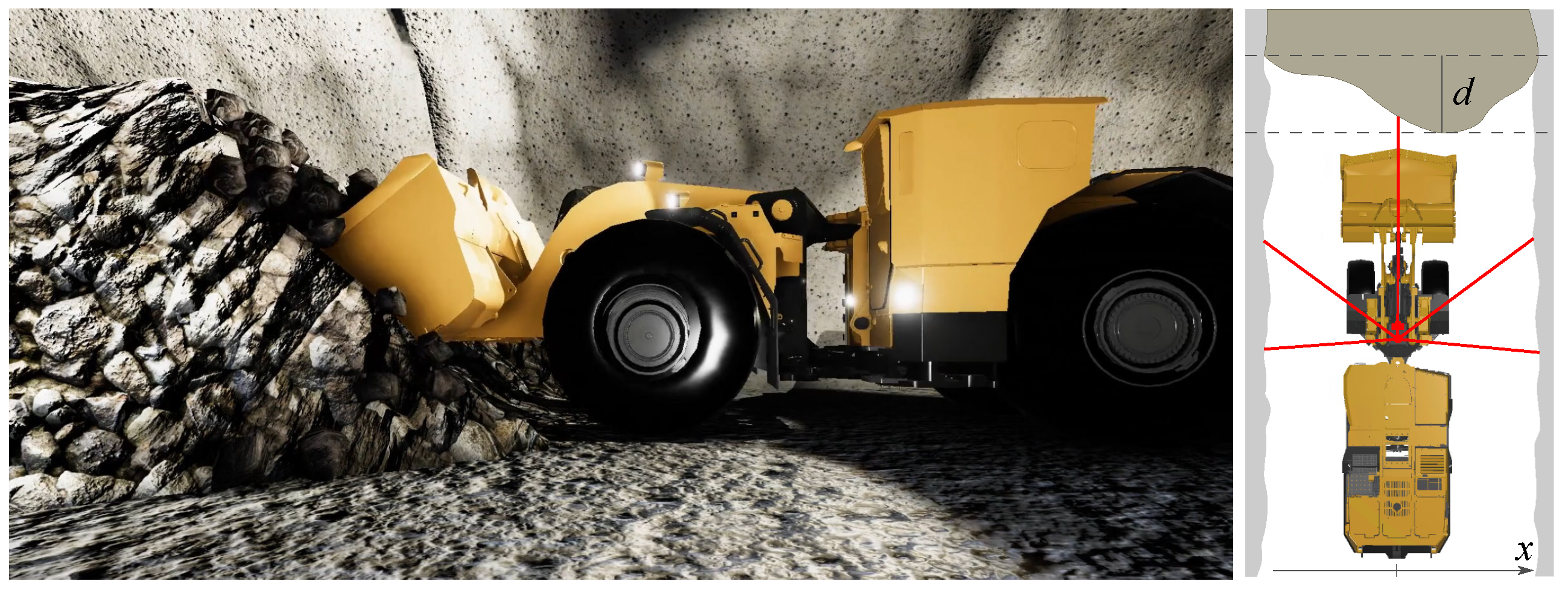
The simulated environment consisted of an LHD and a narrow underground drift with a muck pile (see
Figure 1 and the
Supplementary Video Material). The environment was created in Unity [
24] by using a physics plugin, AGX Dynamics for Unity [
25,
26]. The vehicle model consisted of a multibody system with a drivetrain and compliant tires. The model was created from CAD drawings and data sheets of the ScoopTram ST18 from Epiroc [
27]. It consisted of 21 rigid bodies and 27 joints, of which 8 were actuated. The mass of each body was set to match the 50-tonne vehicle’s center of mass. Revolute joints were used to model the waist articulation, wheel axles, and bucket and boom joints; prismatic joints were used for the hydraulic cylinders with ranges that were set according to the data sheets.
The drivetrain consisted of a torque curve engine, followed by a torque converter and a gearbox. The power was then distributed to the four wheels through a central-, front-, and rear-differential system. The torque curve and gear ratios were set to match the data of the real vehicle. The hoisting of the bucket was controlled by a pair of boom cylinders, and the tilting was controlled by a tilt cylinder and Z-bar linkage. The hydraulic cylinders were modeled as linear motor constraints, and the maximum force was limited by the engine’s current speed. That is, a closed-loop hydraulic system was not modeled.
The drift was 9 m wide and 4.5 m tall with a rounded roof. The muck pile was modeled using a multiscale real-time model [
26] that combined continuum soil mechanics, discrete elements, and rigid multibody dynamics for realistic dig force and soil displacement.
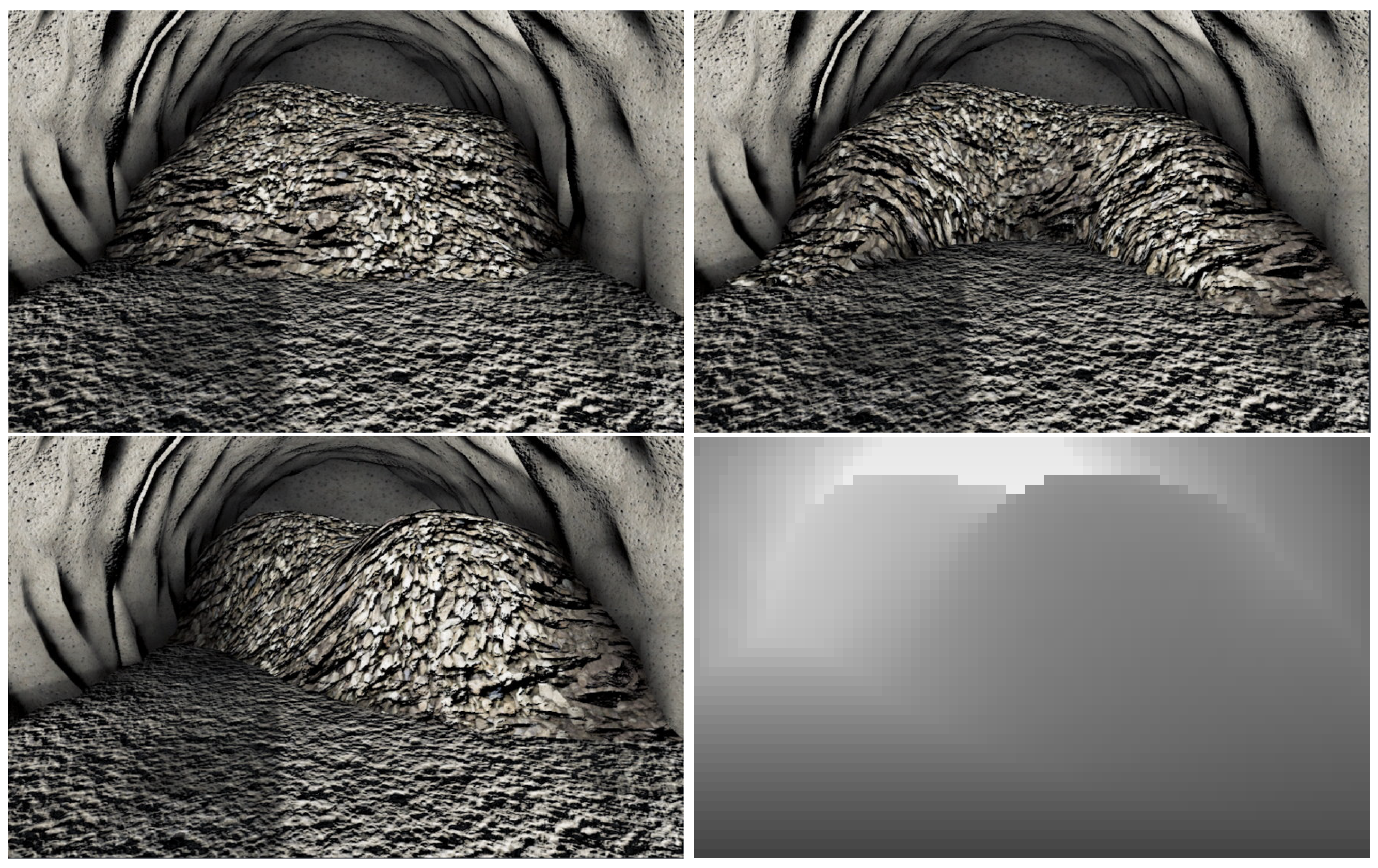
The sample piles observed by the cameras on the vehicle are shown in
Figure 2. The LHD was also equipped with 1D lidar, which measured the distance to the tunnel walls and the pile in five directions, as shown in
Figure 1.
The muck was modeled with a mass density of 2700 kg/m3, internal friction angle of 50°, and cohesion of 6 kPa. Natural variations were represented by adding a uniform perturbation of ±200 kg/m3 to the mass density, with random penetration force scaling ranges that were between 5 and 8 for each pile. Variations in the sample piles’ shapes were ensured by saving the pile shape generations. After loading 10 times from an initial pile, the new shape was saved into a pool of initial pile shapes and tagged as belonging to generation 1. A state inheriting from generation 1 was tagged as generation 2, and so on.
The simulations ran with a 0.02 s timestep and the default settings for the direct iterative split solver in AGX Dynamics [
25]. The grid size of the terrain was set to 0.32 m.
4. DRL Controller
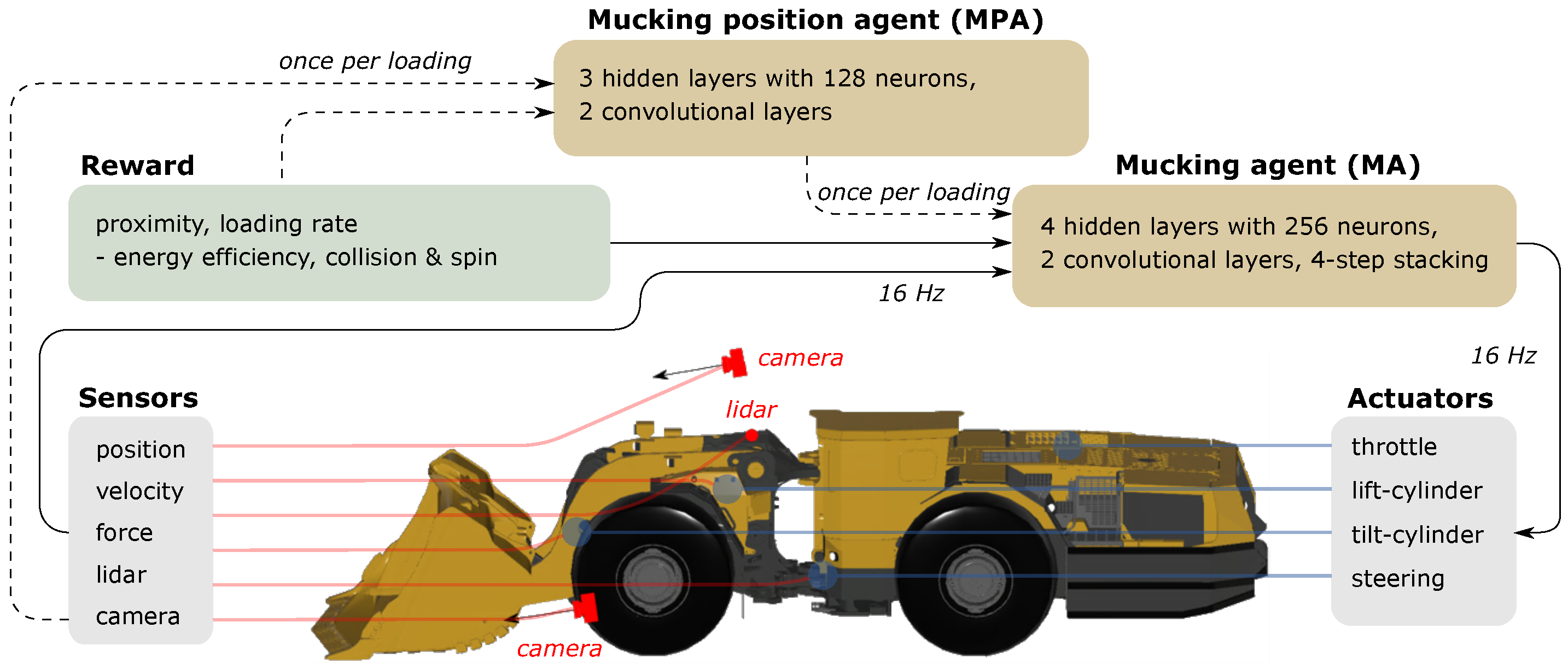
The task of performing several consecutive mucking trajectories requires long-term planning of how the state of a muck pile develops. Training a single agent to handle both high-level planning and continuous motion control was deemed to be too difficult. Therefore, two cooperating agents were trained—a mucking position agent (MPA) and a mucking agent (MA). The former chose the best mucking position—once for each loading cycle—and the latter controlled the vehicle at 16 Hz to efficiently muck at the selected position. To train the agents, we used the implementation of the soft actor–critic (SAC) algorithm [
28] in ML-Agents [
29,
30], which followed the implementation in Stable Baselines [
31], and we used the Adam optimization algorithm. SAC is an off-policy DRL algorithm that trains the policy,
, to maximize a trade-off between the expected return and the policy entropy, as seen in the following augmented objective function:
where
r is the reward for a given state–action pair,
and
, at a discrete timestep
t. The inclusion of the policy entropy in the objective function with weight factor
(a hyperparameter) contributes to the exploration during training and results in more robust policies that generalize better to unseen states. Combined with off-policy learning, this makes the SAC a sample-efficient DRL algorithm, which will be important for the MPA, as explained below.
Figure 3 illustrates the relation between the two agents. The MPA’s observations are from a depth camera at a fixed position in the tunnel with a resolution 84 × 44. The action is to decide on the lateral position in the tunnel at which to dig into the pile. This decision is made once per loading.
The MA’s task is to complete a mucking cycle. This involves the following: approaching the pile to reach the mucking position while the vehicle is straight for maximum force and avoiding collision with the walls; filling the bucket by driving forward and gradually raising and tilting the bucket while avoiding slipping of the wheels; deciding to finish and break out by tilting the bucket to the maximum and holding it still. The MA observes the pile by using depth cameras, which were simulated by using a rendered depth buffer, and lidar data, which were simulated by using line-geometry intersection, in addition to a set of scalar observations consisting of the positions, velocities, and forces of the actuated joints, the speed of the center shaft, and the lateral distance between the bucket’s tip and the target mucking position. The scalar observations were stacked four times, meaning that we repeated observations from previous timesteps, thus giving the agent a short-term “memory” without using a recurrent neural network. The actions included the engine throttle, and the target velocities of each hydraulic cylinder controlled the lift, tilt, and the articulated steering of the vehicle. Note that the target velocity is not necessarily the actual velocity achieved by the actuator due to limited power available and resistance from the muck.
The MA’s neural network consisted of four hidden fully connected layers of 256 neurons each. The depth camera data were first processed by two convolutional layers, followed by four fully connected layers, where the final layer was concatenated together with the final layer for the scalar observations. The MPA’s neural network differed only in the fully connected layers, where we instead used three layers with 128 neurons each. Both the MA and the MPA were trained with a batch size of 256, a constant learning rate of 10
−5, a discount factor of
= 0.995, an update of the model at each step, and the initial value of the entropy coefficient
in Equation (
1) set to
. The buffer size was reduced from
for the MA and to 10
5 for the MPA. These network designs and hyper-parameters were found by starting from the default values in the ML agents and testing for changes that led to better training. There was probably room for further optimization.
The MA reward function depends on how well the selected mucking position was achieved, the rate of bucket filling, and the work exerted by the vehicle. The complete reward function is
where
decays with the lateral deviation of
from the target mucking position, and
is the increment in the bucket’s filling fraction
l over the last timestep. If the vehicle came into contact with the wall or if a wheel was spinning, this was registered with two indicators that were set to
and
, respectively. Otherwise, these had a value of 1. The work
p done by the engine and the hydraulic cylinders for tilting, lifting, and steering since the previous action was summed to
. The weight factors
and
J
−1 were set to make the two terms in Equation (
2) dimensionless and similar in size. The reward favored mucking at the target position and the increase in the volume of material in the bucket compared to the previous step while heavily penalizing collision with walls and spinning of the wheels. Finally, subtracting the current energy consumption encouraged energy-saving strategies and mitigated unnecessary movements that did not increase the possibility of current or future material in the bucket.
Additionally, a bonus reward was given if the agent reached the end state. The bonus reward was the final position reward multiplied by the final bucket filling fraction:
This encouraged the agent to finish the episode when it was not possible to fill the bucket any further, except by reversing and re-entering the pile.
The MPA received a reward for each loading completed by the MA. The reward was the final filling fraction achieved by the mucking agent multiplied by a term that promoted keeping a planar pile surface,
, where
d is the longitudinal distance between the innermost and outermost points on the edge of the pile, as shown in
Figure 1, and
m. The reward became
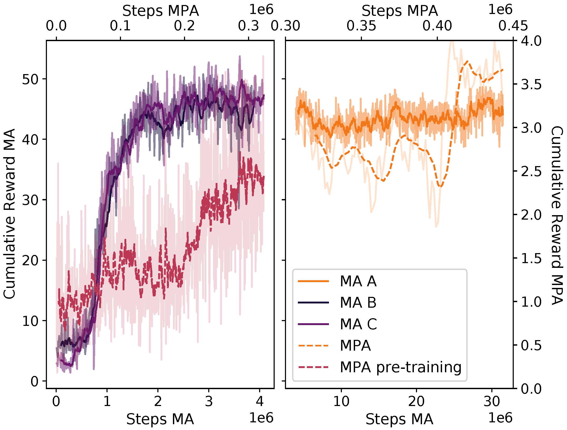
Due to the comparatively slow data collection, it is important to use a sample-efficient DRL algorithm. The two agents were trained in two steps—first separately and then together. The mucking agent was trained with a curriculum setup, using three different lessons. Each lesson increased the number of consecutive loading trajectories by five—from 10 to 20—and the number of pile shape generations by 1—from 0 to 2. During pre-training, each trajectory targeted a random mucking position on the pile. The MPA was first trained with the pre-trained MA without updating the MA model. When the MPA showed some performance, we started updating the MA model together with the MPA model. The model update rate for both models was then limited by the MPA model.
With the SAC, the model was updated at each loading action (16 Hz). The computational time for doing this was similar to that of running the simulation, which was roughly in real time. Hence, training over 30 million steps corresponded to roughly 500 CPU hours. We did not explore the possibility of speeding up the training process by running multiple environments in parallel.
5. Results
We measured the performance of the DRL controller in three different configurations, which are denoted as A, B, and C. Controller A combined the MPA and MA with the reward functions (
2) and (
4), while controllers B and C mucked at random positions instead of using the MPA. For comparison, controller C did not include the penalty for energy usage in Equation (
2). The training progress is summarized in
Figure 4. Controllers B and C were trained for the same number of steps and using the same hyper-parameters, while A continued to train from the state at which B ended.
For each controller, we collected data from 953 individual loadings. Each sample was one out of twenty consecutive loadings starting from one of the four initial piles. The pile was reset after twenty loadings. During testing, the muck pile parameters are set to the default values, except for the mass density, which was set to the upper limit so that one full bucket was about 17.5 t. The loaded mass was determined from the material inside the convex hull of the bucket. This ensured that we did not overestimate the mass in the bucket by including material that might fall off when backing away from the pile.
The mucking agents learned the following behavior, which is also illustrated in the
Supplementary Video Material. The mucking agent started by lining up the vehicle towards the target mucking position, with the bucket slightly raised from the ground and tilted upwards. When the vehicle approached the mucking pile, the bucket was brought flat to the ground and driven into the pile at a speed of approximately 1.6 m/s. Soon after entering the pile, the MA started lifting and tilting the bucket. This increased the normal force, which provided traction in order to continue deeper into the pile without the wheels slipping. After some time, the vehicle started breaking out of the pile with the bucket fully tilted.
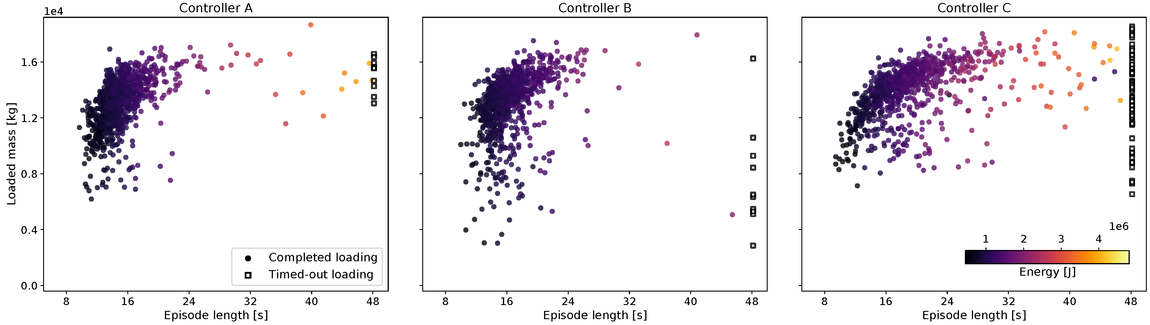
The mass loaded into the bucket at the end of each episode is plotted in
Figure 5 with the corresponding episode duration and energy use. The majority of the trajectories are clustered in the upper-left corner of high productivity (t/s). Each of the three controllers had some outliers, loadings with low mass, and/or long loading times. If the mucking agent did not reach the final state of breaking out with the bucket fully tilted within 48 s, the loading was classified as failed. The common reason for timing out was the vehicle being stuck in the pile with a load that was too large to break out. Controller C, which was not rewarded for being energy efficient, had a longer loading duration and was more prone to getting stuck.
The mean productivity and energy usage for controllers A, B, and C are presented in
Table 1. For reference, we have also added the performance of an experienced driver manually operating an ST14 loader [
13], with the loaded mass re-scaled to the relative bucket volume of the ST18 loader,
, while keeping the loading time and energy per unit mass the same. The failure ratio and mucking position error are also included. Comparing controllers B and C, we observe that the energy penalty in the reward functions leads to 21% lower energy consumption, a 7% increase in productivity, and a reduction of the failure ratio from 7% to 1%. We conclude that controllers A and B learned a mucking strategy that actively avoided entering states that would lead to high energy consumption and delayed breaking out. On average, the loaded mass was between 75 and 80% of the vehicle’s capacity of 17.5 t. The energy usage was 1.4–1.9 times larger than the energy required for raising the mass by 4 m. This is reasonable considering the soil’s internal friction and cohesion and that the internal losses in the LHD were not accounted for.
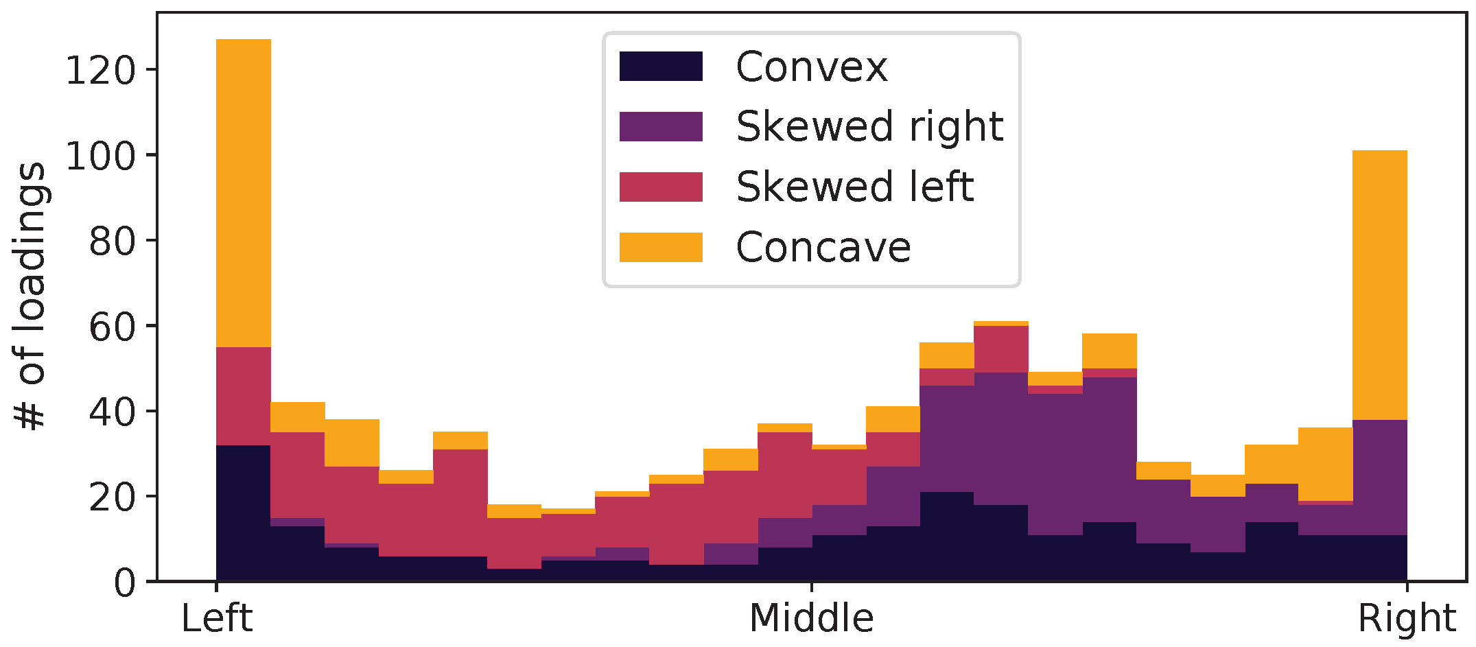
Controller A had 9% higher productivity than controller B, which mucked at random positions, and used 4% less energy. This suggests that the mucking position agent learned to recognize favorable mucking positions from the depth images. Confirming this,
Figure 6 shows the distribution of the mucking positions for the four different initial piles that were shown in
Figure 2. For the left-skewed pile, the MPA chose to muck more times on the left side of the tunnel, presumably because that action allowed the filling of the bucket with a smaller digging resistance, and it left the pile in a more even shape. The same pattern was true for the pile that was skewed to the right. For the concave pile, the majority of the targets were at the left or right edge, effectively working away the concave shape. For the convex shape, the mucking positions were more evenly distributed.
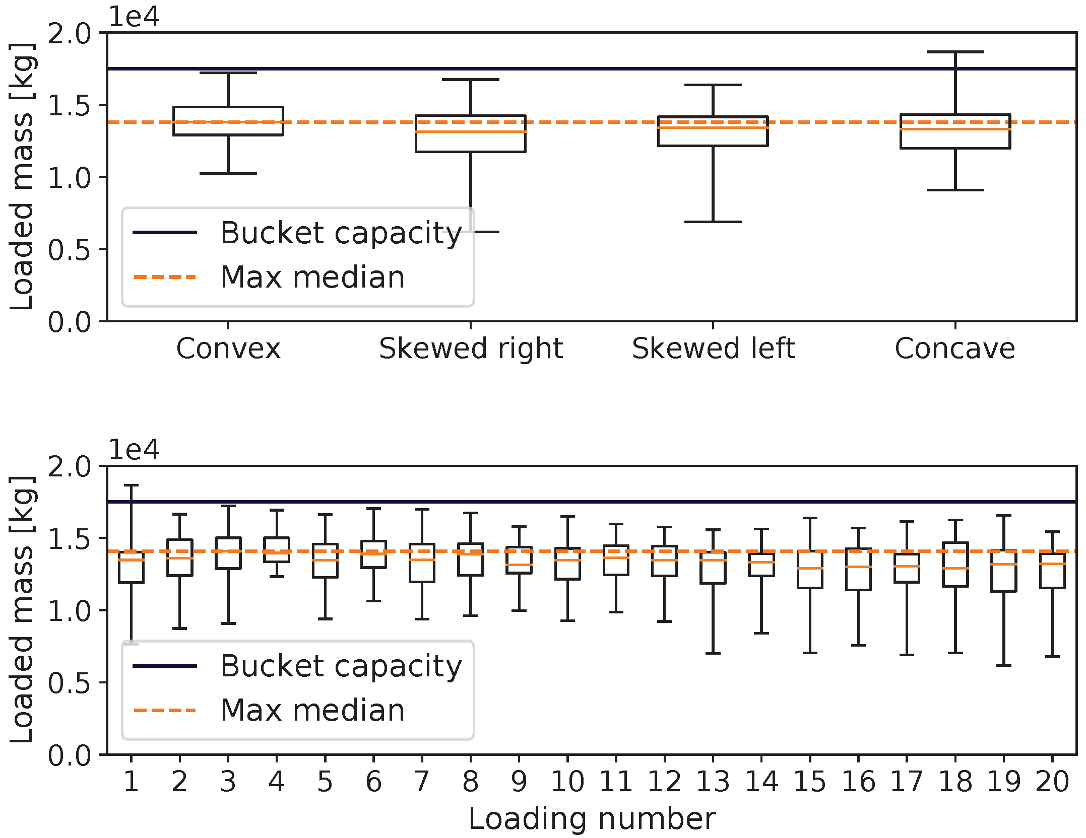
Figure 7 shows the evolution of the loaded mass when using controller A over a sequence of 20 repeated muckings from the initial piles. There was no trend of degradation of the mucking performance. This shows that the MPA acted to preserve or improve the state of the pile and that the DRL controller was generalized to the spaces of different mucking piles.
The target mucking position chosen by the MPA was not guaranteed to be the position at which the LHD actually mucked, as we expected an error in MA’s precision, and it was able to weigh the importance of mucking at the target position against the importance of filling the bucket with a low energy cost. The mean difference between the target and actual mucking positions for controller A was m, which was 0.4% of the bucket’s width.
Compared to the manual reference included in
Table 1, the DRL controllers reached a similar or slightly larger average loading mass, but with higher consistency (less variation) and shorter loading times. The productivity of controller A was 70% higher than that of the manual reference, with an energy consumption that was three times smaller. On the other hand, the DRL controller underperformed relative to the automatic loading control (ALC) in ST14 field tests [
13]. The ALC reached its maximal loading mass with a productivity that was roughly two times greater than that of the DRL controller, but with four times larger energy consumption per loaded tonne. There are several uncertainties in these comparisons, however. The performance of the DRL controller was measured over a sequence of twenty consecutive loadings from the same pile in a narrow drift, thus capturing the effect of a potentially deteriorating pile state. It is not clear whether the ALC field test in [
13] was conducted in a similar way, or if the loadings were conducted on piles prepared in a particular state. There are also uncertainties regarding the precise definition of the loading time and whether the assumed scaling from ST14 to ST18 holds. In future field tests, the amount of spillage on the ground and the slipping of the wheels should also be measured and taken into account when comparing the overall performance. Comparison with [
21] and [
18] is interesting but difficult because of the large differences in the vehicles’ size and strength and the materials’ properties. The reinforcement learning controller in [
21] achieved a fill factor of 65%, and the energy consumption was not measured. The neural network controller in [
18], which was trained by learning from demonstration, reached 81% of the filling of the bucket relative to manual loading, but neither loading time nor work was reported.
7. Conclusions
We found that it is possible to train a DRL controller to use high-dimensional sensor data from different domains without any pre-processing as input for neural network policies in order to solve the complex control task of repeated mucking with high performance. Even though the bucket is seldom filled to the maximum, it is consistently filled with a good amount. It is common for human operators to use more than one attempt to fill the bucket when the pile’s shape is not optimal, which is a tactic that was not considered here.
The inclusion of an energy consumption penalty in the reward function can distinctly reduce the agent’s overall energy usage. This agent learns to avoid certain states that inevitably lead to high energy consumption and the risk of failing to complete the task. The two objectives of loading more material and using less energy were competing, as seen in
Table 1 with controller C’s higher mass and controller A’s lower energy usage. This is essentially a multi-objective optimization problem that will have a Pareto front of possible solutions with different prioritizations between the objectives. In this work, we prioritized by choosing the coefficients
and
in Equation (
2), but future work could analyze this trade-off in more detail.
A low-resolution depth camera observation of a pile’s surface is enough to train the MPA to recognize good 1D positions for the MA to target. By choosing the target position, the overall production increases and the energy consumption decreases compared to when random positions are targeted. Continuing to clear an entire pile by using this method—essentially cleaning up and reaching a flat floor—could be an interesting task for future work.


 ,
, 


