CAD-Based 3D-FE Modelling of AISI-D3 Turning with Ceramic Tooling

Abstract

In this study, the development of a 3D Finite Element (FE) model for the turning of AISI-D3 with ceramic tooling is presented, with respect to four levels of cutting speed, feed, and depth of cut. The Taguchi method was employed in order to create the orthogonal array according to the variables involved in the study, reducing this way the number of the required simulation runs. Moreover, the possibility of developing a prediction model based on well-established statistical tools such as the Response Surface Methodology (RSM) and the Analysis of Variance (ANOVA) was examined, in order to further investigate the relationship between the cutting speed, feed, and depth of cut, as well as their influence on the produced force components. The findings of this study point out an increased correlation between the experimental results and the simulated ones, with a relative error below 10% for most tests. Similarly, the values derived from the developed statistical model indicate a strong agreement with the equivalent numerical values due to the verified adequacy of the statistical model.

1. Introduction

The investigation of machining operations is a topic with increasing interest, especially in the past decades. As the technology involved in the manufacturing industry evolves, the machining-related area of research expands with similar pace. One advancement that many researchers have benefited from, is the Finite Element Method (FEM). With the aid of the latest Finite Element Analysis (FEA) software, it is possible to simulate many machining operations, including the most complicated ones. A number of studies that exist in the bibliography have successfully implemented FEM, modelling this way drilling, milling, turning, and similar processes with adequate approximation. Such studies usually investigate the produced cutting forces, the chip morphology, the distribution of the developed temperatures, the cutting tool wear, as well as the material behavior. The implementation of FEM in machining enables the testing of a wide variety of materials under a significant number of cutting conditions combinations, by minimizing at the same time the experimental work. Therefore, it is possible to save time, reduce costs, and proceed to the manufacturing stage more efficiently.

Klöcke et al. [1] simulated the high speed orthogonal turning of AISI 1045 steel in two dimensions. Authors reported that despite the assumptions that have to be made, the comparison of the simulated and the experimental results showed good agreement. Similarly, Elkaseer et al. [2] employed 2D-FEM to investigate the chip formation and surface morphology during precision turning of 316L steel. The findings of the research reported good agreement between the experiments and FEM, allowing for the identification of the optimum cutting conditions. Ali et al. [3] presented a review on the implementation of FEM during machining of titanium alloy Ti-6Al-4V. Authors stated that the majority of the used FEA software yielded results in high correlation with the equivalent experimental ones, exceeding 90% in many cases. Xiong et al. [4] studied the chip formation process during the orthogonal cutting of TiB₂/7050Al composite, along with the strain rate and the developed temperatures with the aid of 2D-FEM. More similar researches prove that the use of FEM can become a valuable asset when investigating typical machining results such as the tool/chip contact temperatures [5], the chip formation mechanisms [6,7], and the generated cutting forces, as well as the tool wear mechanisms [8,9,10,11].

According to Arrazola et al. [12], the 3D-FEM enabled by high-end computing systems provide better visualization and understanding of the cutting operations. Drilling is the one cutting process that has been widely studied with the use of 3D-FEM [13,14,15,16,17,18]. Due to the nature of the drilling process and the complexity of the tools involved, three-dimensional simulations proved to be valuable assets when studying the phenomena that occur during drilling. Steel, titanium alloys, aluminium alloys, and composites are the most common material families that the researchers select for their studies. Moreover, the study topics usually include measuring of the thrust forces and torques, recording of the chip evolution and morphology, as well as the tool wear conditions. Additionally, measuring the developed temperatures and the induced stresses is another important subject that has been studied with the aid of FEM.

Similarly, milling and micro-milling was studied with the utilization of FEM in three dimensions [19,20,21,22,23,24,25]. Considering the complex geometry of the tools and the kinematics [26] that develop during the process, the use of 3D is justified. Depending on the parameters investigated, in some cases the use of 2D is sufficient, but most of the time the need to fully represent the problem requires the enabling of all three dimensions. Therefore, it is obvious that parameters such as the full chip morphology, the developed forces in all axes, and the temperature distribution in three dimensions cannot be studied without 3D-FEM.

With the same success, 3D-FEM has been implemented in a number of studies related to the turning operation. Guo and Liu [27] developed a practical 3D-FE analysis model to analyze the turning of hardened AISI-52100 steel using a PCBN tool. Authors incorporated the thermo-mechanical properties of the workpiece material and additionally, proposed an improved friction model determined by force calibration and material tests. Valiorgue et al. [28] proposed a new methodology for predicting residual stresses induced in the finish turning of AISI304L without modelling the chip removal process, which speeds up the calculation stage. Moreover, authors investigated the interactions between each revolution of the turning process. Later, Malakizadi et al. [29] presented an approach based on FEM, for predicting the flank wear for uncoated cemented carbide inserts during the conventional turning. Buchkremer et al. [30] proposed a new model of final ductile fracture for the 3D-FE simulation of chip breakage in the turning process of AISI-1045, along with a new non-iterative calibration procedure. Magalhães et al. [31] established a FE model for hard turning examining the effects of multi-chamfered edges on tool wear and residual stresses. Tzotzis et al. [32] investigated the performance of ceramic inserts in terms of the micro-geometry (nose radius and cutting edge type) with the aid of 3D-FE modelling. Authors have stated that the increased correlation between the numerical and equivalent experimental results allowed for the development of a statistically-based prediction model for the resultant turning force.

The present paper investigates the effects of standardized cutting conditions such as the cutting speed, the feed, and the depth of cut on the generated machining forces induced during the AISI-D3 steel hard turning. Four levels of cutting conditions were selected in order to increase the research range. In addition, a typical industry-rated turning insert (SNGA family) was chosen as the cutting tool for the study. Due to the increased number of tests that occurred, a design of experiments was prepared with the Taguchi method in order to reduce both the required number of simulation runs and the computational time. The development of the Finite Element (FE) model and the numerical simulations were carried out with the DEFORM™-3D version 12 FEA software. Furthermore, a comparison between the numerical results and the experimental ones, which are available in the literature [33], was conducted to validate the established FE model. Finally, the Response Surface Methodology (RSM) was utilized to develop a prediction model for the resultant turning force with respect to the prepared design of experiments and based on the yielded numerical results. Furthermore, the Analysis of Variance was employed to verify the developed statistical model.

2. Materials and Methods

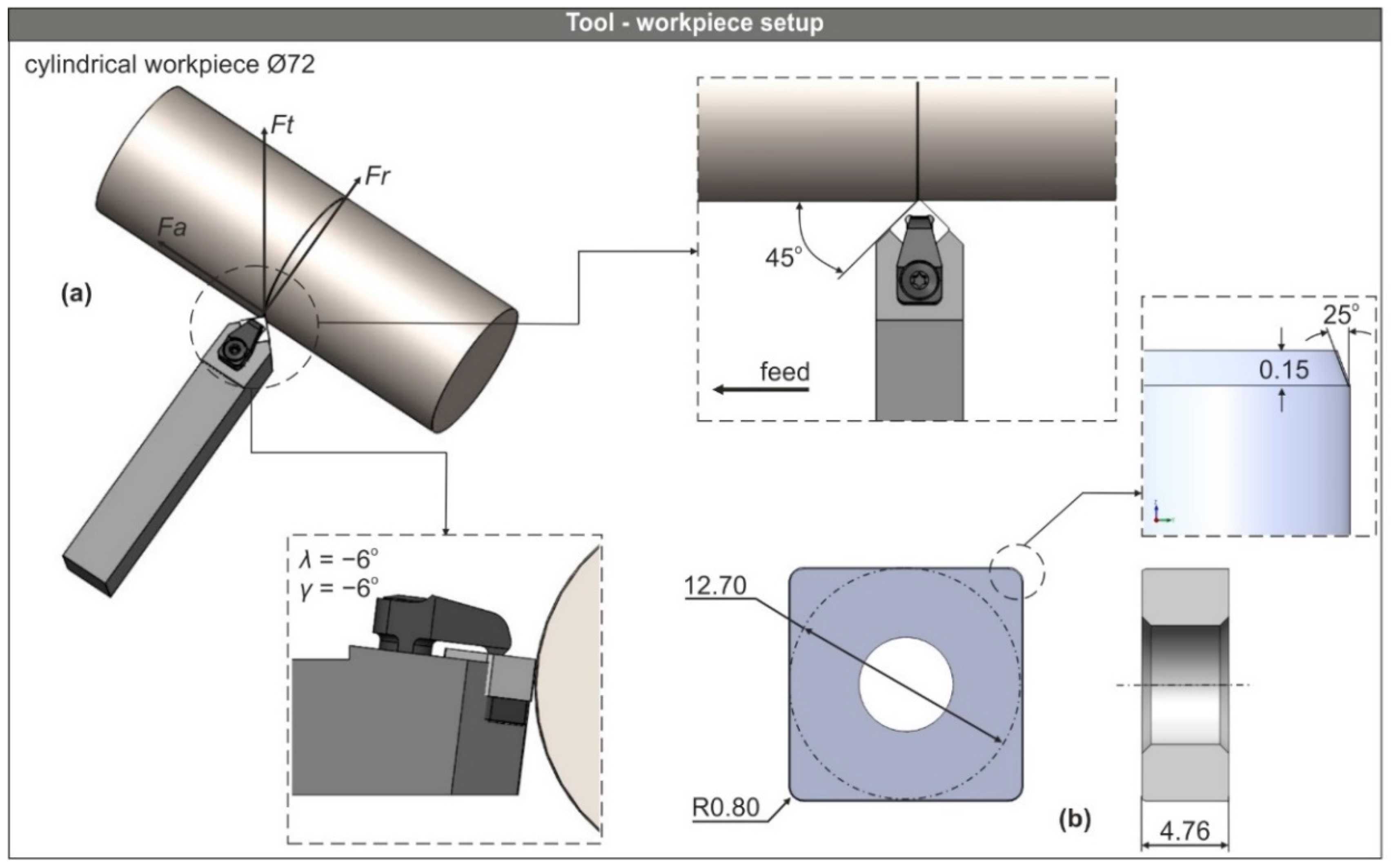
2.1. Framework of the Turning Process

A simplified version of the turning process setup was prepared with the aid of SolidWorks™ 2018 focusing on the cutting zone. The tool assembly used in the present study consists of a tool-holder and an industry-standard square shaped insert. The ISO reference number of the tool-holder is CSDNN2525M12 and the corresponding code for the tool is the SNGA120408T01525 mixed alumina insert. The workpiece was designed as a cylinder with a diameter of 72 mm. Moreover, the selected material for the workpiece is the AISI-D3 steel.

Figure 1 depicts the CAD-based setup of the process. Specifically, Figure 1a illustrates both the workpiece and the tool models along with the generated cutting forces: F_t denotes the tangential force, F_r is the radial force, and F_a represents the feed force. In addition, Figure 1a includes two schematics that depict the position of the cutting insert and the feed direction. The position of the tool is defined with respect to the cutting angles which are inherited from the tool-holder and its geometry. Therefore, the lead angle is k_r = 75° and both the rake (γ) and inclination angle (λ) are negative and equal to −6°. Finally, Figure 1b contains the full geometry of the tool.

In the present study, the effects of three cutting parameters combined on four levels were investigated. The factors and their ranges were selected based on previous investigations [33,34]. The levels of the factors and their values are summarized in

Table 1. Process inputs and levels of the finite element (FE) model.

Level	Vc (m/min)	f (mm/rev)	ap (mm)
I	75	0.08	0.10
II	105	0.12	0.20
III	150	0.16	0.30
IV	210	0.20	0.40

.

By combining these factors and their levels, a set of N = 4³ = 64 experiments would occur. Due to the increased number of experiments, the Taguchi method was implemented in order to reduce the experiments number and thus save time and resources. This method is considered a robust parameter design, which can be used for the product or process design that enables the minimizing of variation and sensitivity to noise. Several researchers have successfully used the Taguchi method during their manufacturing-related studies [35,36,37]. In this study, the four-level design with three factors (V_c, f, and a_p) produces an L₁₆ orthogonal array, which leads to 16 experiments. Orthogonal arrays are design matrices that contain the factor settings used in the design of experiments to equally consider all levels of all factors. The signal-to-noise ratio (S/N) formula used in this design is nominal-the-best, which is represented by Equation (1). The S/N ratio is a measure of how a response varies relative to the nominal value under different noise conditions and is calculated for all combinations.

$$\frac{S}{N}=10\log \frac{\overline{y}}{{{\displaystyle S}}_y^2}$$

(1)

where $\overline{y}$ is the mean of the responses for a given factor level combination and $S_y^2$ is the standard deviation of the responses for the same factor level combination. The factor settings for the 16 runs required in the present investigation are discussed in Section 3.1.

2.2. D-FE Model Setup

With the aid of the CAD-based setup of the turning process, the tool-workpiece system was defined in such a way that the problem was simplified in terms of the analysis domain. The point of this simplification is to achieve reasonable simulation times. First, the tool-holder model was eliminated from the tool assembly and only the insert model was used. Furthermore, the round steel bar model was converted to an arc-shaped part. The arc has a 20° angle and belongs to a circle with a diameter of 72 mm (Figure 2a). In addition, the workpiece was designed partially cut based on the used depth of the cut (Figure 2b), to reduce computational costs.

2.2.1. Definition of the Analysis Interface

A designer application [38] was used to generate the CAD model of the tool, including the full geometry. In contrast, the workpiece model was designed with SolidWorks™ 2018 based on the used depth of cut, the tool nose radius, and the steel bar diameter. At the pre-processing stage, the workpiece was modelled as deformable and meshed with approximately 32,000 to 60,000 tetrahedral elements depending on the value of the feed. The minimum element size of the mesh was set to 25% of the feed [39,40]. Moreover, a 7:1 ratio between the largest and the smallest element size of the mesh was applied to the section of the workpiece (see Figure 2b), so that the solid elements of the workpiece that participate in the removal process are created seven times smaller compared to the rest of the elements. Additionally, the default remeshing technique of DEFORM™-3D ensured that the mesh at the area of interest, retained an adequate number of elements each time new chips were formed. On the other hand, the tool was modelled as rigid and meshed with approximately 76,000 elements. Similarly to the workpiece, the area at the tool tip which is in contact with the workpiece, was refined with a 4:1 size ratio (see Figure 2c). The default values for the mesh size ratio for both the workpiece and the tool were utilized.

To simulate the cutting process, the workpiece’s model was fixed, whereas the cutting tool was allowed to follow the cutting path, as indicated in Figure 2a. In addition to the translational boundary conditions, the heat exchange due to the convection and conduction between the workpiece and the tool were also set. The value for both heat transfer coefficients, which were used in the presented model, are the ones suggested by DEFORM™ [41]. Specifically, h_conv = 0.02 N/(s × mm × °C) for dry cutting and h_cond = 45 N/(s × mm × °C).

2.2.2. Modelling of Material Behavior

In order to simulate the material flow stress for the workpiece, the Johnson-Cook model was applied. This model is preferred when the high strain, strain rate, and temperatures occur in the machining process mainly due to simplicity and ease-of-use. Equation (2) represents the model and can be divided into three modules: The first relates to the strain hardening properties of the material, the second one to the strain rate sensitivity, and the last one to the thermal softening properties.

$$\sigma =\left(A+B{\epsilon }^n\right)\left(1+C\ln \frac{\dot{\epsilon }}{{\dot{\epsilon }}_0}\right)\left[1-{\left(\frac{T-T_0}{T_m-T_0}\right)}^m\right]$$

(2)

where σ is the equivalent stress, A, B, and C are the initial yield stress, the strain hardening modulus, and the strain rate dependence coefficient, respectively, ε denotes the plastic strain, n represents the strain hardening exponent, m represents the thermal softening coefficient, $\dot{\epsilon }$ is the plastic strain rate, whereas ${\dot{\epsilon }}_0$ is the reference plastic strain rate, consequently T, T₀, and T_m are the temperatures involved in the model, the reference temperature, the ambient temperature, and the melting temperature, respectively.

Table 2. The Johnson-Cook model constants for the AISI-D3 steel [41].

A (MPa)	B (MPa)	C	n	m	T0 (°C)	Tm (°C)
1985.6	193	0.1524	0.2768	0.2852	20	1421

presents the flow stress constants for the AISI-D3 steel, which were adapted from the material’s flow stress diagrams found in the software’s library.

Moreover,

Table 3. Thermo-mechanical properties for the tool [42] and the workpiece [41].

Mechanical Properties	AISI-D3	Ceramic
Young’s Modulus Ε (GPa)	206.75	415
Density ρ (kg/m3)	7700	3500
Poisson’s ratio γ	0.30	0.22
Hardness (HRC)	63	−
Thermal Properties	AISI-D3	Ceramic
Heat capacity (J/kgK)	381.26 @100 °C 429.90 @300 °C 555.42 @600 °C	334
Thermal expansion (μm/mK)	12.0	8.4
Thermal conductivity (W/mK)	50.71 @100 °C 45.69 @300 °C 33.94 @600 °C	7.5

contains the thermo-mechanical properties which were used in the numerical study. Both the thermal conductivity and the heat capacity were expressed as a function of temperature f(Temp). In addition, a reference strain rate equal to 1/s was employed.

In order to approximate the fracture of the material that occurs due to the material separation under the action of stress, the normalized Cockcroft-Latham damage model was employed. This model has been used in many early studies [43,44,45]. Equation (3) represents the modified criterion developed by Cockcroft and Latham [46]. In this formula, the maximum principal stress is normalized by the effective stress.

$$D_c={\displaystyle \underset{0}{\overset{{\epsilon }_f}{\int }}\frac{{\sigma }_{\max }}{\overline{\sigma }}}d{\epsilon }_{pl},$$

(3)

In the integral, D_c is the critical value of the fracture damage, σ_max and $\overline{\sigma }$ denote the maximum tensile principal stress and the effective stress accordingly, ε_f represents the limit fracture strain, and ε_pl is the plastic strain.

According to Agmell [47], the contact interface between the cutting tool and the workpiece can be divided into three discrete zones: The sticking, the adhesive, and the sliding. The latter in particular, plays a major role when studying the machining of steel and in most cases the approximation of the developed friction stresses in this zone is sufficient when modelling friction. In order to simplify the modelling procedure, Coulomb’s law was utilized for the estimation of the aforementioned stresses according to Equation (4) [47].

$${\tau }_f=\mu {\sigma }_n,$$

(4)

where τ_f is the frictional shear stress, μ is the shear friction coefficient, and finally, σ_n denotes the tool-chip interface stress. Studies related to the machining of steel [48,49] suggest using a value of friction coefficient between 0.5 and 0.6 in general. Since these values are also proposed by DEFORM™, the friction coefficient was set to 0.6 for the presented simulation runs.

3. Results and Discussion

3.1. FEM-Based Results of the Machining Forces

Figure 3 illustrates three sample forces vs. time diagrams. In particular, Figure 3a illustrates the force vs. time diagram for the radial force (F_r), Figure 3b for the tangential force (F_t), and finally, Figure 3c for the feed force (F_a) which were generated during turning of the AISI-D3 steel with the SNGA120408T01525 tool. The following cutting conditions apply for the obtained results: V_c = 210 m/min, f = 0.12 mm/rev, and a_p = 0.30 mm. The diagrams point out that the force increases rapidly as soon as the edge of the tool touches the uncut surface of the workpiece until the steady state phase is reached where the force maintains a steady mean value. To keep simulation times low, only a small part of the workpiece was cut. When the tool completes its pass on the workpiece and the material removal process ends, the force quickly decreases until it reaches zero. Even though the total time of the process is relatively low, the high number of time steps (approximately 2900 for this case) ensured the establishment of the steady state.

The default remeshing technique was applied in order to keep the minimum required amount of elements. For this, some spikes occurred during the simulation processes. In order to minimize the effect of the spikes on the calculated force values, the first order exponential smoothing provided by the software was enabled. Furthermore, in order to calculate the mean values of the generated cutting forces, the obtained data were exported to Excel™ and the average function was used on the values of each one of the steady state datasets.

In addition, Figure 3d depicts the evolution of the chip for the aforementioned cutting conditions. The forming of the chip follows a rather expected shape, proving the success of the FE modelling. The same chip morphology was found for the total of the simulation tests.

The complete set of the simulations were prepared and executed, with respect to the L₁₆ orthogonal Taguchi array. The design of experiments along with the results for each run are presented in

Table 4. FE model results for the force components.

Cutting Parameters				Simulated Cutting Forces
Standard Order	Vc (m/min)	f (mm/rev)	ap (mm)	Fr (N)	Ft (N)	Fa (N)	Fresultant (N)
1	75	0.08	0.10	193.2	85.1	35.4	214.1
2	75	0.12	0.20	269.5	118.8	74.6	303.8
3	75	0.16	0.30	426.4	206.4	106.2	485.5
4	75	0.20	0.40	489.2	302.6	164.7	598.3
5	105	0.08	0.20	262.1	95.8	70.8	287.9
6	105	0.12	0.10	209.4	78.6	36.4	226.6
7	105	0.16	0.40	465.7	275.4	159.7	564.1
8	105	0.20	0.30	421.1	208.6	112.3	483.2
9	150	0.08	0.30	332.6	126.8	118.9	375.3
10	150	0.12	0.40	405.9	212.1	158.8	484.7
11	150	0.16	0.10	204.1	98.7	38.4	229.9
12	150	0.20	0.20	324.5	152.6	63.4	364.2
13	210	0.08	0.40	327.8	159.5	145.6	392.5
14	210	0.12	0.30	312.1	160.3	98.6	364.5
15	210	0.16	0.20	287.6	132.4	61.3	322.5
16	210	0.20	0.10	217.2	94.9	36.4	239.8

.

By observing the simulated results for the turning force components presented in Table 4, it is concluded that the radial force is the governing component contributing to the resultant machining force between 66.8 and 85.4% of the total value, depending on the depth of cut. In general, the lower the value of depth of cut, the higher the percentage of contribution. Additionally, the depth of cut has a significant impact on the generated forces. Particularly, as the depth of cut increases so does the cutting force, for example, the increase between the test number 8 and 4 (the depth of cut shifts from 0.30 to 0.40 mm) is calculated as approximately 23.8%. A similar trend can be observed for the full range of the cutting parameters.

Similar cutting conditions were applied in the work of Quiza et al. [37], during the investigation of AISI-D2 turning with the CNGA120408T0120 ceramic tool at a 0.2 mm depth of cut. Moreover, Aouici et al. [34] used similar cutting parameters for machining of the AISI-H11 steel with the SNGA120408S01020 insert at depths of cut between 0.15 and 0.45 mm. Additionally, they reported findings related to the influence of the cutting conditions and the contribution of the components, which comply with the ones presented in this study. Moreover, the way the feed and cutting speed influence the machining force components induced during turning of AISI-D3, are discussed in the experimental work of Aouici et al. [33] verifying the findings of the present investigation. In the aforementioned experimental work, the lathe used is TOS TRENCIN (model SN40C-spindle power 6.6 kW) and the test workpiece was hardened to a value equal to 63 HRC through quenching at 940 °C and tempering at 280 °C.

3.2. Statistically-Based Analysis of Machining Forces

The established FE model allowed for the development of a prediction model based on statistical methodologies. This way, the FE model can be validated, as well as the future experimental work on turning of AISI-D3 can be minimized. The RSM was chosen for this case, as it is a proven tool which is employed by many researchers for several purposes, such as optimization of machining conditions and prediction of cutting forces [40,50,51,52]. With respect to the L₁₆ design, which includes the three factors and the four levels, the results from the 16 simulation runs were used for the development of the statistical model. The generated model is a second order polynomial which is represented by Equation (5). Due to the fact that the relationship between the input variables and the output variable (response) is non-linear, the polynomial describing the model includes linear, quadratic, and cross-product terms. Therefore, Y is the response of the model (resultant machining force), a₀ represents the fixed term, X_i are the input variables (cutting speed, feed, and depth of cut) and b_i, b_ij, b_ii are the vectors that contain the regression coefficients (linear, quadratic, and cross-product, accordingly).

$$Y=a_0+{\displaystyle {\sum }_{i=1}^n{b}_i{X}_i+{\displaystyle {\sum }_{i,j}^n{b}_{ij}{X}_i{X}_j+}}{\displaystyle {\sum }_{i=1}^n{b}_{ii}{X}_i^2},$$

(5)

Using the results which are presented in Table 4, the previously mentioned formula can be adapted to represent the statistically-based prediction model (Equation (6)).

$$F_{resultant}=59.7+0.41V+234f+994a_p-0.00178V^2-1031f^2-229{a_p}^2+1.42Vf-1.78V{a}_p+2408f{a}_p$$

(6)

In Equation (6), F_resultant is the resultant machining force in N, whereas V, f, and a_p are the cutting speed (m/min), the feed (mm/rev), and the depth of cut (mm), respectively.

The results for the calculated resultant machining force yielded by both the numerical and the statistical model, as well as the experiments are presented in

Table 5. Comparison of the resultant machining force.

	Fresultant (N)			Relative Error (%)
Standard Order	Simulated	Experimental	Predicted	Predicted vs. Simulated	Predicted vs. Experimental
1	214.1	197.8	204.1	−4.65	3.17
2	303.8	318.8	327.2	7.69	2.62
3	485.5	472.3	461.6	−4.91	−2.25
4	598.3	622.3	607.5	1.53	−2.38
5	287.9	295.2	298.0	3.50	0.93
6	226.6	214.5	221.6	−2.22	3.27
7	564.1	589.5	558.3	−1.02	−5.28
8	483.2	505.9	484.5	0.28	−4.23
9	375.3	360.6	365.6	−2.58	1.38
10	484.7	503.9	489.7	1.02	−2.82
11	229.9	213.1	235.2	2.29	10.37
12	364.2	383.3	361.9	−0.63	−5.59
13	392.5	415.1	391.8	−0.20	−5.62
14	364.5	384.6	368.5	1.10	−4.19
15	322.5	345.3	318.0	−1.39	−7.91
16	239.8	230.2	240.4	0.24	4.45

. Moreover, a comparison between the results is made, indicating a strong correlation between the predicted and the numerical results, as well as between the predicted and the experimental. Particularly, the relative error was estimated below 10% for all cases, with the exception of test number 11 (predicted vs. experimental), which was calculated as 10.37%.

Figure 4 graphically compares the relative error percentage between the values of resultant turning force derived from the statistical model and the experiments, in addition to the statistical model vs. the numerical model. It is highlighted that the relative error between the simulated and the predicted values are in general higher compared to the ones derived from the experimental vs. the predicted. This is more clear for tests number 7, 8 and 11 to 16. Despite this observation, the relative error is low for both cases (below 10%) with the exception of test number 11.

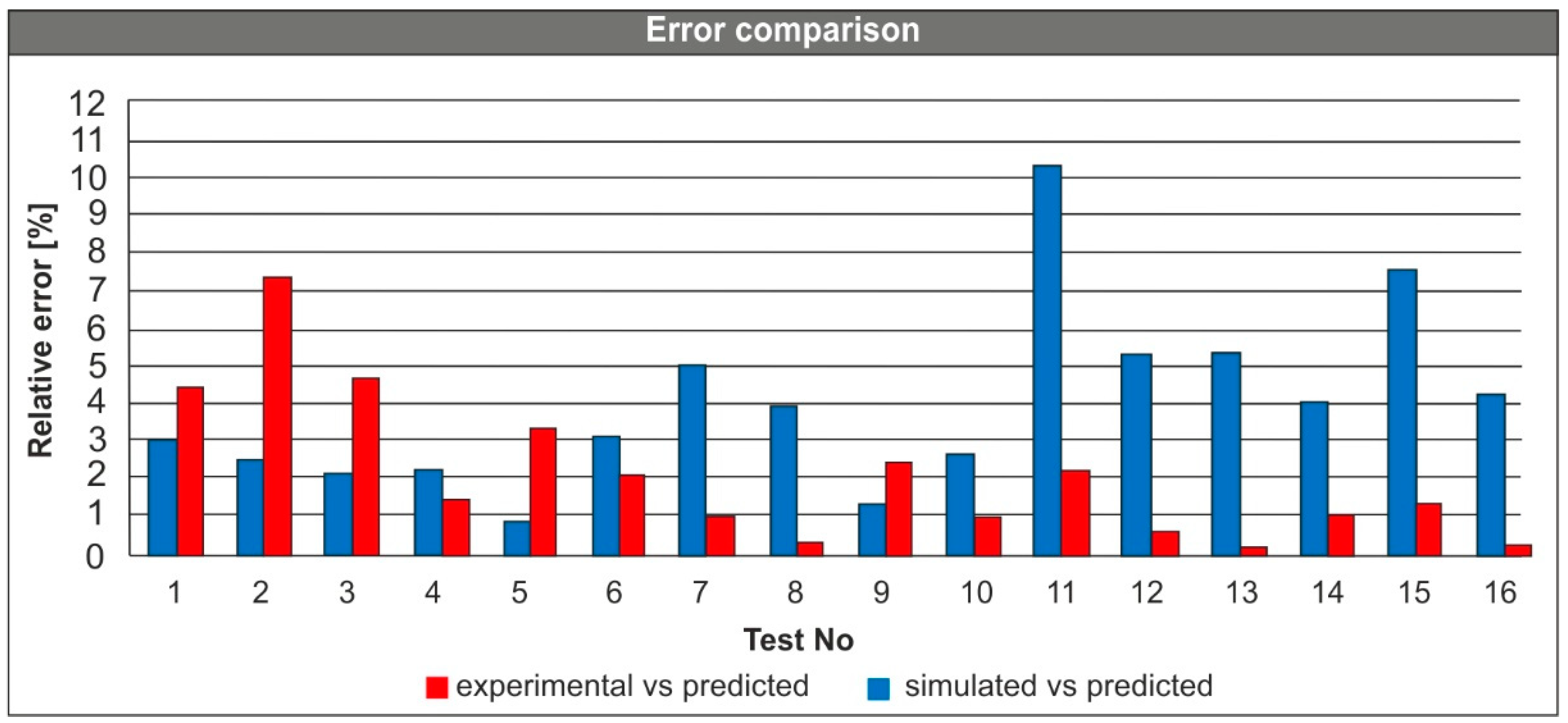
3.3. Model Validation Results

The produced model was tested for its validity with the employment of the Analysis of Variance (ANOVA). A standard significance level equal to 0.05 was set in order to test the fit of the model. The results showed an adjusted R-squared of 98.17% proving the fit. In addition to the sum of squares and the mean square of the test,

Table 6. ANOVA results for the resultant machining force.

Source	Degree of Freedom	Sum of Squares	Mean Square	f-Value	p-Value
Regression	9	222,884	24,764.9	90.24	0.000
Residual Error	6	1647	274.4
Total	15	224,531
R-sq (adj) = 98.17%
Term	PE Coefficient	SE Coefficient	t-Value	p-Value
Constant	59.7	95.7	0.62	0.556
V	0.41	0.953	0.43	0.682
f	234	910	0.26	0.805
ap	994	332	2.99	0.024
V2	−0.00178	0.00218	−0.82	0.445
f2	−1031	2588	−0.40	0.704
ap2	−229	414	−0.55	0.601
V × f	1.42	3.33	0.43	0.686
V × ap	−1.78	1.33	−1.33	0.231
f × ap	2408	1417	1.70	0.140

contains the factors involved in the modelling procedure, along with their contribution. By observing Table 6, it is highlighted that the depth of cut contributes the most, since its p-value is below 0.05. This fact, clearly indicates the strong influence of the depth of cut to the generated forces. Moreover, the validity of the model is enhanced by its p-value (0.000).

Figure 5 graphically presents the residual analysis results. Particularly, Figure 5a illustrates the normal probability plot which highlights if any of the data points is far from the fit line. In the present analysis, no serious departures are visible. Figure 5b shows the residuals vs. the fitted values plot which clearly indicate that the residuals are almost evenly scattered on both sides of the reference line. Figure 5c contains the residual histogram which highlights the residual distribution in the system, according to Figure 5c, a residual uniformity is present in the system. Finally, the overall normality of the system can be proved by Figure 5d which depicts the residuals vs. the order of the data, no specific pattern can be recognized in the graph, a fact that proves the absence of systematic faults in the system.

As a final step, the 3D surface plots (Figure 6) were designed according to the polynomial solutions in order to illustrate the combined effect of the cutting speed, the feed, and the depth of cut to the generated cutting forces. The values of the used parameters were drawn from within the range which is studied in the present investigation. Finally, the following conclusions can be drawn by observing the 3D plots:

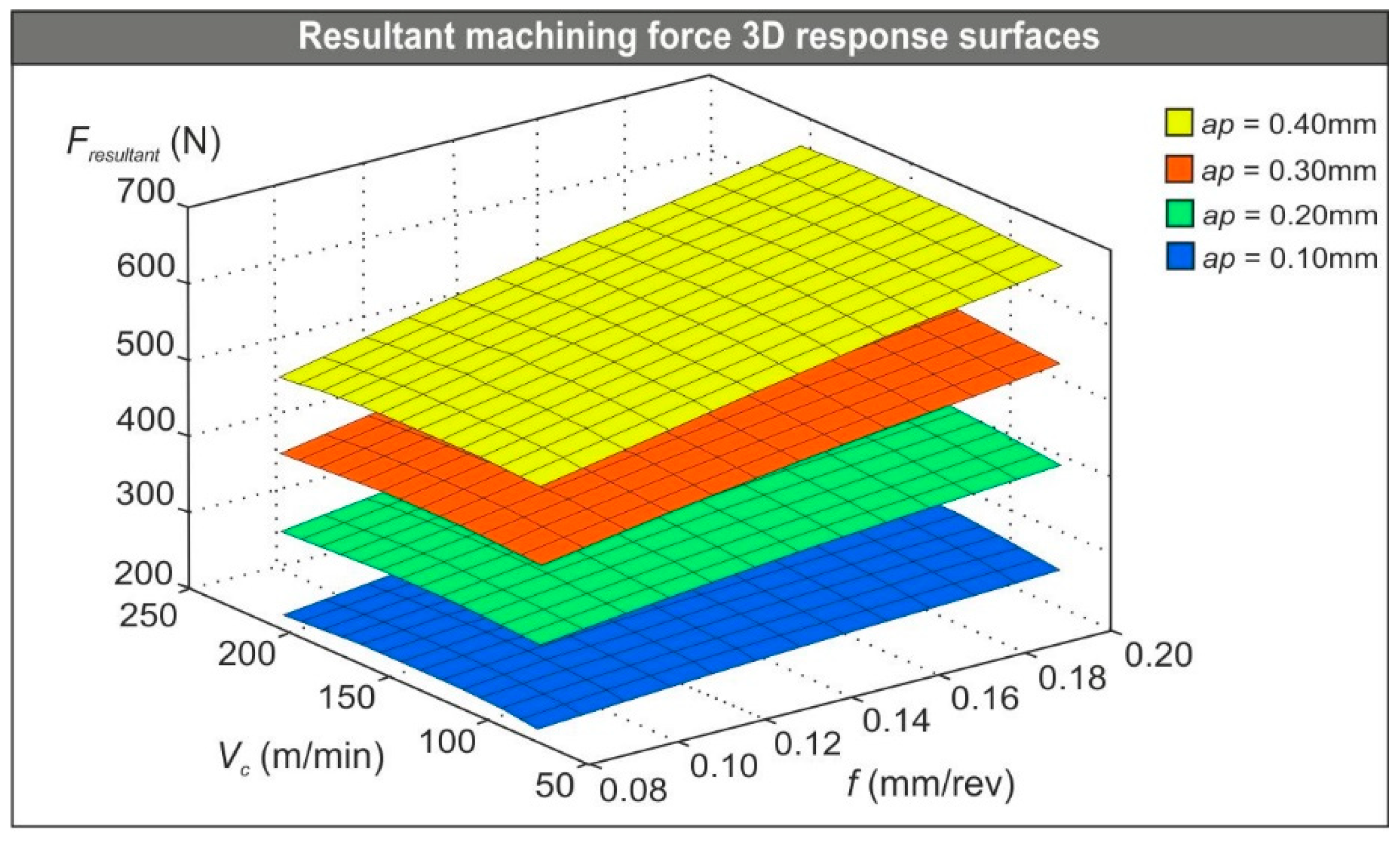
• Depth of cut is clearly the dominant parameter of the three and has the strongest effect on the resultant force. Actually, the produced forces are almost tripled as the depth of cut increases from the lowest value (0.10 mm) to the maximum (0.40 mm).
• Any increase in the feed acts to increase the resultant machining force. The level of increase is notable, especially as the tool cuts deeper.
• Lastly, the cutting speed seems to have a marginal influence on the F_resultant. Despite this fact, a small increase is present at speeds between 100 and 150 m/min.

4. Conclusions

In the present study, both the 3D-FE modelling procedure of AISI-D3 turning with the SNGA120408 tool and the establishment of a statistically-based prediction model for the induced machining forces are presented. In addition to the aforementioned models, an effort is made to investigate the performance of the cutting tool with respect to industry-standard cutting conditions. In order to verify the obtained results, a comparison is made between the numerical values of the cutting force components and the equivalent experimental ones which are available in the bibliography, as well as between the simulated results and the predicted ones. Furthermore, an additional verification of the prediction model is made via the ANOVA. Finally, the findings of this paper can lead to the following conclusions:

• The radial force is the component that affects the most the resultant machining force, contributing to the total value by up to 85%. It is noted that the contribution percentage is higher at lower values of the depth of cut.
• As the feed rise acts to increase the resultant machining force significantly, this trend is notable as the tool cuts deeper. On average, a shift from 0.08 to 0.20 mm/rev would increase F_resultant by about 44.5, 48.6, 56, and 25% at the depth of cut equal to 0.40, 0.30, 0.20, and 0.10 mm, respectively.
• Similarly, the depth of cut has a strong impact on the generated machining forces. Specifically, F_resultant would rise on average by approximately 55, 33.3, and 25% in the case of the changing depth of cut from 0.10 to 0.20 mm, 0.20 to 0.30 mm, and finally, 0.30 to 0.40 mm, accordingly.
• Finally, the influence of the cutting speed on the generated machining force is minimal. A slight increase in the F_resultant is noticeable near the intermediate values of the cutting speed.

References

1. Klocke, F.; Raedt, H.-W.; Hoppe, S. 2D-FEM simulation of the orthogonal high speed cutting process. Mach. Sci. Technol. 2001, 5, 323–340. [Google Scholar] [CrossRef]
2. Elkaseer, A.; Abdelaziz, A.; Saber, M.; Nassef, A. FEM-based study of precision hard turning of stainless steel 316L. Materials 2019, 12, 2522. [Google Scholar] [CrossRef] [PubMed] [Green Version]
3. Ali, M.H.; Ansari, M.N.M.; Khidhir, B.A.; Mohamed, B.; Oshkour, A.A. Simulation machining of titanium alloy (Ti-6Al-4V) based on the finite element modeling. J. Brazilian Soc. Mech. Sci. Eng. 2014, 36, 315–324. [Google Scholar] [CrossRef]
4. Xiong, Y.; Wang, W.; Jiang, R.; Lin, K.; Shao, M. Mechanisms and FEM simulation of chip formation in orthogonal cutting in-situ TiB2/7050Al MMC. Materials 2018, 11, 606. [Google Scholar] [CrossRef] [Green Version]
5. Saez-de-Buruaga, M.; Soler, D.; Aristimuño, P.X.; Esnaola, J.A.; Arrazola, P.J. Determining tool/chip temperatures from thermography measurements in metal cutting. Appl. Therm. Eng. 2018, 145, 305–314. [Google Scholar] [CrossRef]
6. Ye, G.G.; Chen, Y.; Xue, S.F.; Dai, L.H. Critical cutting speed for onset of serrated chip flow in high speed machining. Int. J. Mach. Tools Manuf. 2014, 86, 18–33. [Google Scholar] [CrossRef]
7. Shuang, F.; Chen, X.; Ma, W. Numerical analysis of chip formation mechanisms in orthogonal cutting of Ti6Al4V alloy based on a CEL model. Int. J. Mater. Form. 2018, 11, 185–198. [Google Scholar] [CrossRef]
8. Chen, G.; Ren, C.; Yang, X.; Jin, X.; Guo, T. Finite element simulation of high-speed machining of titanium alloy (Ti-6Al-4V) based on ductile failure model. Int. J. Adv. Manuf. Technol. 2011, 56, 1027–1038. [Google Scholar] [CrossRef]
9. Yanda, H.; Ghani, J.A.; Haron, C.H.C. Application of FEM in investigating machining performance. Adv. Mater. Res. 2011, 264–265, 1033–1038. [Google Scholar] [CrossRef]
10. Calamaz, M.; Coupard, D.; Girot, F. A new material model for 2D numerical simulation of serrated chip formation when machining titanium alloy Ti-6Al-4V. Int. J. Mach. Tools Manuf. 2008, 48, 275–288. [Google Scholar] [CrossRef] [Green Version]
11. Chiappini, E.; Tirelli, S.; Albertelli, P.; Strano, M.; Monno, M. On the mechanics of chip formation in Ti-6Al-4V turning with spindle speed variation. Int. J. Mach. Tools Manuf. 2014. [Google Scholar] [CrossRef] [Green Version]
12. Arrazola, P.J.; Özel, T.; Umbrello, D.; Davies, M.; Jawahir, I.S. Recent advances in modelling of metal machining processes. CIRP Ann. Manuf. Technol. 2013, 62, 695–718. [Google Scholar] [CrossRef]
13. Tzotzis, A.; Markopoulos, A.; Karkalos, N.; Kyratsis, P. 3D finite element analysis of Al7075-T6 drilling with coated solid tooling. MATEC WEb Conf. 2020, 318, 1–6. [Google Scholar] [CrossRef]
14. Oezkaya, E.; Hannich, S.; Biermann, D. Development of a three-dimensional finite element method simulation model to predict modified flow drilling tool performance. Int. J. Mater. Form. 2019, 12, 477–490. [Google Scholar] [CrossRef]
15. Guo, Y.B.; Dornfeld, D.A. Finite element modeling of burr formation process in drilling 304 stainless steel. J. Manuf. Sci. Eng. Trans. ASME 2000, 122, 612–619. [Google Scholar] [CrossRef]
16. Rajesh Jesudoss Hynes, N.; Kumar, R. Simulation and Experimental Validation of Al7075-T651 Flow Drilling Process. J. Chinese Soc. Mech. Eng. 2017, 38, 413–420. [Google Scholar]
17. Gao, X.; Li, H.; Liu, Q.; Zou, P.; Liu, F. Simulation of stainless steel drilling mechanism based on Deform-3D. Adv. Mater. Res. 2011, 160–162, 1685–1690. [Google Scholar] [CrossRef]
18. Nagaraj, M.; Kumar, A.J.P.; Ezilarasan, C.; Betala, R. Finite element modeling in drilling of Nimonic C-263 alloy using deform-3D. Comput. Model. Eng. Sci. 2019, 118, 679–692. [Google Scholar] [CrossRef]
19. Thepsonthi, T.; Grul Özel, T. 3-D finite element process simulation of micro-end milling Ti-6Al-4V titanium alloy: Experimental validations on chip flow and tool wear. J. Mater. Process. Technol. 2015, 221, 128–145. [Google Scholar] [CrossRef]
20. Maurel-Pantel, A.; Fontaine, M.; Thibaud, S.; Gelin, J.C. 3D FEM simulations of shoulder milling operations on a 304L stainless steel. Simul. Model. Pract. Theory 2012, 22, 13–27. [Google Scholar] [CrossRef] [Green Version]
21. Pittalà, G.M.; Monno, M. 3D finite element modeling of face milling of continuous chip material. Int. J. Adv. Manuf. Technol. 2010, 47, 543–555. [Google Scholar] [CrossRef]
22. Nan, X.; Xie, L.; Zhao, W. On the application of 3D finite element modeling for small-diameter hole drilling of AISI 1045 steel. Int. J. Adv. Manuf. Technol. 2016, 84, 1927–1939. [Google Scholar] [CrossRef]
23. Soo, S.L.; Dewes, R.C.; Aspinwall, D.K. 3D FE modelling of high-speed ball nose end milling. Int. J. Adv. Manuf. Technol. 2010, 50, 871–882. [Google Scholar] [CrossRef]
24. Wu, H.B.; Zhang, S.J. 3D FEM simulation of milling process for titanium alloy Ti6Al4V. Int. J. Adv. Manuf. Technol. 2014, 71, 1319–1326. [Google Scholar] [CrossRef]
25. Davoudinejad, A.; Tosello, G.; Parenti, P.; Annoni, M. 3D finite element simulation of micro end-milling by considering the effect of tool run-out. Micromachines 2017, 8, 187. [Google Scholar] [CrossRef] [Green Version]
26. Tapoglou, N.; Antoniadis, A. 3-Dimensional kinematics simulation of face milling. Measurement 2012, 45, 1396–1405. [Google Scholar] [CrossRef]
27. Guo, Y.B.; Liu, C.R. 3D FEA modeling of hard turning. J. Manuf. Sci. Eng. Trans. ASME 2002, 124, 189–199. [Google Scholar] [CrossRef]
28. Valiorgue, F.; Rech, J.; Hamdi, H.; Gilles, P.; Bergheau, J.M. 3D modeling of residual stresses induced in finish turning of an AISI304L stainless steel. Int. J. Mach. Tools Manuf. 2012, 53, 77–90. [Google Scholar] [CrossRef]
29. Malakizadi, A.; Gruber, H.; Sadik, I.; Nyborg, L. An FEM-based approach for tool wear estimation in machining. Wear 2016, 368–369, 10–24. [Google Scholar] [CrossRef]
30. Buchkremer, S.; Klocke, F.; Veselovac, D. 3D FEM simulation of chip breakage in metal cutting. Int. J. Adv. Manuf. Technol. 2016, 82, 645–661. [Google Scholar] [CrossRef]
31. Magalhães, F.C.; Ventura, C.E.H.; Abrão, A.M.; Denkena, B. Experimental and numerical analysis of hard turning with multi-chamfered cutting edges. J. Manuf. Process. 2020, 49, 126–134. [Google Scholar] [CrossRef]
32. Tzotzis, A.; García-Hernández, C.; Talón, J.L.H.; Kyratsis, P. FEM based mathematical modelling of thrust force during drilling of Al7075-T6. Mech. Ind. 2020, 21, 1–14. [Google Scholar] [CrossRef]
33. Bensouilah, H.; Aouici, H.; Meddour, I.; Athmane, M. Performance of coated and uncoated mixed ceramic tools in hard turning process. Measurement 2016, 82, 1–18. [Google Scholar] [CrossRef]
34. Aouici, H.; Yallese, M.A.; Chaoui, K.; Mabrouki, T.; Rigal, J.F. Analysis of surface roughness and cutting force components in hard turning with CBN tool: Prediction model and cutting conditions optimization. Meas. J. Int. Meas. Confed. 2012, 45, 344–353. [Google Scholar] [CrossRef]
35. Benardos, P.G.; Vosniakos, G.C. Prediction of surface roughness in CNC face milling using neural networks and Taguchi’s design of experiments. Robot. Comput. Integr. Manuf. 2002, 18, 343–354. [Google Scholar] [CrossRef]
36. Masmiati, N.; Sarhan, A.A.D. Optimizing cutting parameters in inclined end milling for minimum surface residual— stressTaguchi approach. Measurement 2015, 60, 267–275. [Google Scholar] [CrossRef]
37. Quiza, R.; Figueira, L.; Davim, J.P. Comparing statistical models and artificial neural networks on predicting the tool wear in hard machining D2 AISI steel. Int. J. Adv. Manuf. Technol. 2008, 37, 641–648. [Google Scholar] [CrossRef]
38. Tzotzis, A.; Garcia-Hernandez, C.; Talón, J.L.H.; Kyratsis, P. CAD-based automated design of FEA-ready cutting tools. J. Manuf. Mater. Process. 2020, 4, 104. [Google Scholar] [CrossRef]
39. Tzotzis, A.; Garcia-Hernandez, C.; Talón, J.L.H.; Kyratsis, P. Influence of the nose radius on the machining forces induced during AISI-4140 hard turning: A CAD-based and 3D FEM approach. Micromachines 2020, 11, 798. [Google Scholar] [CrossRef]
40. Tzotzis, A.; Garcia-Hernandez, C.; Talón, J.L.H.; Kyratsis, P. 3D FE Modelling of machining forces during AISI 4140 hard turning. Strojniški Vestn. J. Mech. Eng. 2020, 66, 467–478. [Google Scholar] [CrossRef]
41. Scientific Forming Technologies Corporation. DEFORM, version 11.3 (PC); Documentation; Columbus, OH, USA, 2016. [Google Scholar]
42. Hu, H.J.; Huang, W.J. Tool life models of nano ceramic tool for turning hard steel based on FEM simulation and experiments. Ceram. Int. 2014, 40, 8987–8996. [Google Scholar] [CrossRef]
43. Kobayashi, S.; Lee, C.H. Deformation mechanics and workability in upsetting solid circular cylinders. In Proceedings of the North American Metalworking Research Conference, Ontario, ON, Canada, 14–15 May 1973; Volume 1. [Google Scholar]
44. Oh, S.I.; Chen, C.C.; Kobayashi, S. Ductile fracture in axisymmetric extrusion and drawing—Part 2: Workability in extrusion and drawing. J. Manuf. Sci. Eng. 1979, 101, 36–44. [Google Scholar] [CrossRef]
45. Oyane, M.; Sato, T.; Okimoto, K.; Shima, S. Criteria for ductile fracture and their applications. J. Mech. Work. Technol. 1980, 4, 65–81. [Google Scholar] [CrossRef]
46. Cockcroft, M.G.; Latham, D.J. Ductility and the workability of metals. J. Inst. Met. 1968, 96, 33–39. [Google Scholar]
47. Agmell, M. Applied FEM of Metal Removal and Forming, 1st ed.; Studentlitteratur: Lund, Sweden, 2018; ISBN 978-91-44-12507-7. [Google Scholar]
48. Arrazola, P.J.; Matsumura, T.; Kortabarria, A.; Garay, A.; Soler, D. Finite element modelling of chip formation process applied to drilling of Ti64 alloy. In Proceedings of the 6th International Conference on Leading Edge Manufacturing in 21st Century, LEM, Saitama, Japan, 8–10 November 2011; pp. 1–6. [Google Scholar]
49. Haglund, A.J.; Kishawy, H.A.; Rogers, R.J. An exploration of friction models for the chip-tool interface using an Arbitrary Lagrangian-Eulerian finite element model. Wear 2008, 265, 452–460. [Google Scholar] [CrossRef]
50. Meddour, I.; Yallese, M.A.; Bensouilah, H.; Khellaf, A.; Elbah, M. Prediction of surface roughness and cutting forces using RSM, ANN, and NSGA-II in finish turning of AISI 4140 hardened steel with mixed ceramic tool. Int. J. Adv. Manuf. Technol. 2018, 97, 1931–1949. [Google Scholar] [CrossRef]
51. Kyratsis, P.; Markopoulos, A.; Efkolidis, N.; Maliagkas, V.; Kakoulis, K. Prediction of thrust force and cutting torque in drilling based on the response surface methodology. Machines 2018, 6, 24. [Google Scholar] [CrossRef] [Green Version]
52. Efkolidis, N.; Hernández, C.G.; Talón, J.L.H.; Kyratsis, P. Modelling and prediction of thrust force and torque in drilling operations of Al7075 using ANN and RSM methodologies. Strojniški Vestn. J. Mech. Eng. 2018, 64, 351–361. [Google Scholar] [CrossRef]
Figure 1. (a) The Computer Aided Design (CAD) based tool-workpiece setup and (b) the model of the SNGA120408T01525 insert.
Machines 09 00004 g001
Figure 2. (a) The FE model setup, (b) the analysis domain, and (c) the meshed tool.
Machines 09 00004 g002
Figure 3. Sample force vs. time diagrams for 0.30 mm depth of cut, 210 m/min cutting speed, and 0.12 mm/rev feed; (a) radial force component, (b) tangential force component, (c) feed force component, and (d) the evolution of the chip for the same conditions.
Machines 09 00004 g003
Figure 4. Relative error comparison between the simulated, predicted, and experimental results.
Machines 09 00004 g004
Figure 5. Residual analysis graphs: (a) Probability plot, (b) residuals vs. fitted values, (c) residual histogram, and (d) residuals vs. order.
Machines 09 00004 g005
Figure 6. Three-dimensional (3D) plots of the resultant turning force based on the polynomial solutions for each depth of cut.
Machines 09 00004 g006