1. Introduction
Vision systems are largely employed to impart an additional sense to robotic systems. A class of vision systems are the depth cameras that are devices able to acquire depth information (in the three-dimensional space) along with bi-dimensional (RGB) images [
1]. The quality of their acquisition is strongly affected by the device cost. Low-cost depth sensors, such as stereo triangulation, structured light and time-of-flight (TOF) cameras, have found use in many vision applications such as object/scene recognition, human pose estimation and gesture recognition [
2,
3]. Several works have been proposed to track the motion of objects or human body parts, especially hands, by means of visual devices [
4,
5]. Moreover, the combination of computer vision with artificial intelligence and gesture recognition algorithms has used for computer–human interaction [
6,
7]. The applicability of these devices requires the development of proper algorithms mainly based on image segmentation, artificial intelligence, neural networks and machine learning tools. Depending on application and device, vision-based methods can be employed for qualitative tracking and/or high-precision measurements.
Using Kinect V2, a low-cost camera, we have already shown the possibility of using vision data for measuring the displacement of a mechanical system employing colored markers [
8].
In the robotics field, the kinematics of a prosthetic finger has been quantified employing vision systems such as Digital Image Correlation [
9,
10,
11,
12] and Microsoft Kinect V2 [
13].
A further step could be the mechanical or robotic system control through vision system aids. In autonomous driving, we find vehicles equipped with numerous sensors (not only multiple cameras but also other kinds of sensors) able to perceive their surroundings [
14,
15]. Advanced control systems interpret sensory information and identify appropriate navigation paths, as well as obstacles and relevant signage [
16]. Ferreira et al. [
17] have shown the application of computer vision systems for position control and trajectory planning of a mobile robot. Cueva et al. [
18] have presented control of an industrial robot using computer vision to aid people with physical disabilities in daily working activities through gesture recognition. Calli et al. [
19] have used vision feedback to develop predictive model control to obtain precise manipulation of under-actuated hands. Pagano et al. [
20] have recently shown the applicability of an RGB-D sensor to reconstruct the path for a flexible gluing process in shoe industry.
In this paper, we shall explain how to steer and control the movement of a mechanical system through the information acquired through only one camera. In this specific case, we have used an RGB-D sensor, the Intel Realsense®, as the vision device and a linear actuator as the mechanical system.
The paper is divided in three parts. We will firstly provide the description of algorithms able to give reliable measurements of the mechanical system displacement and object recognition. Afterwards, two control applications with vision-based feedback will be shown: the first one is target object tracking while the second one is a ball equilibrium task.
The object is recognized through a color segmentation algorithm. Acting like a human eye, the camera dictates the movements of the actuator stroke.
As a future perspective, the assessment of such methodologies could aid the development of other more complex vision-based strategies to control other kinds of mechanical systems.
The activity described in this paper constitutes the development of the one presented at the Third International Conference of IFToMM Italy (IFIT 2020): Cosenza, C., Nicolella, A., Niola, V., Savino, S. RGB-D vision device for tracking a moving target. In Advances in Italian Mechanism Science: Mechanisms and Machine Science 91, pp.841–848 Springer, Cham, Switzerland, 2021 [
21].
2. Experimental Setup
The test bench (
Figure 1) includes a linear actuator (Gliderforce LACT4P-12V-05, Pololu
®, Las Vegas NV, USA) connected to a control board (JRK 21v3, Pololu
®, Las Vegas NV,) and a vision device (Intel
® Realsense™ D435, Intel
®, Santa Clara CA, USA).
The selected mechanical system has a 120 mm stroke (100 mm usable) and a feedback potentiometer. The stroke step-size is 10 mm in order to fit a target value line comparable with the experimental value line obtained by using the vision device. The target value line is the theoretical target value; i.e., the value that comes out of the following equation:
The goes from 0 to 4095 that is the value required for the control board to move the linear actuator and reach the (i.e., the distance from 0 to 100 mm). To measure the repeatability, five tests were done. The camera device captures the point cloud data of the object. The point cloud data contains the points of the external surface object in the three-dimensional space. Intel® Realsense™ D435 is an active stereo camera which means it actively utilizes a light such as a laser or a structured light to make easier the stereo matching problem. These types of cameras use feedback from the image flows to control camera parameters. The camera specification requires an operating range of 0.11–10 m. We performed all the proposed experiments at approximately 500 mm ± 50 mm from the camera.
3. Methodology
The methodology aimed to track a target object using a vision system. Vision data, acquired through an RGB-D device, were used for target object recognition and position control of the mechanical system. To reach this goal, we assessed two main procedures: the first allowed us to recognize the target object and compute its position; the second one measured the actuator stroke position through vision data.
3.1. Target Object Detection
The target object was recognized in the RGB image through color segmentation. Afterwards, from the pixels selected in the RGB matrix, the algorithm extracted the target object position in the point-cloud finding its 3D coordinates. The alignment between depth and RGB matrix was performed through the SDK 2.0 developed for Intel
® Realsense™ D435 and all the cameras of the D400 series (available at
https://www.intelrealsense.com/developers/). For the first application, the target object tracking once the object was shaped in the 3D space, the algorithm computed the closest point position to the piston that would be used as input command for the actuator movement.
For the second application, the ball equilibrium task, the algorithm again detected the points belonging to the red ball (of which the radius was known), then computed a sphere fitting procedure and found the ball center. Subsequently, the ball center was used as input command in the control application.
3.2. Measuring Actuator Stroke Position through Vision Devices
Since the points acquired through the vision system had a cylindrical shape (gray dots in
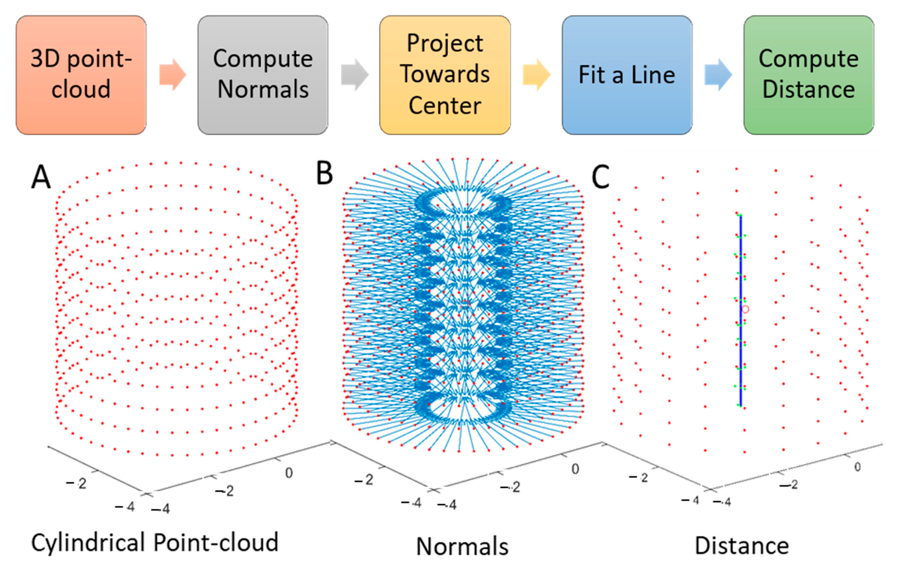
Figure 2), we proposed an algorithm to compute the actuator displacement through some simple geometrical transformations and a linear fitting procedure.
The flowchart in
Figure 3 summarizes the main steps of the algorithm.
For each actuator stroke position, the algorithm performed the following instructions:
- (1)
For each point (
Figure 3A) acquired through the vision system, compute the normal and flip it towards the center (blue arrows in
Figure 3B).
- (2)
Project the points, along the normal, towards a common line that is the cylinder axis (
Figure 3C).
- (3)
Fit these points with a line and compute the distance between the two external points (
Figure 3C).
The algorithm steps that we present in
Figure 3 are an idealization for a case in which the whole external surface can be acquired. However, the algorithm is still able to work using a partial cylinder surface, as in our specific case. The knowledge of the cylinder radius is mandatory, in our code, since it is the projection distance that must be applied to the external points along the normals toward the center.
The results for measurement algorithm, over five independent tests, are reported in
Table 1 and graphically represented in
Figure 4 for ten discrete positions of the actuator stroke (see Experimental Setup section for input settings).
To ensure the algorithm’s performance, we have computed two parameters: the average distance of the values from the target value line, which is 2.83 mm, and the average standard deviation between the five test repetitions, which is 0.35 mm. The first indicator is a statement of the measurement reliability, while the second causes the measurement repeatability. Both the indexes indicate appreciable results of the measuring algorithm, since they indicate an average deviation lower than half a centimeter that it is acceptable for the application we propose. It is worth noting that the first measurements overestimate the target values because the algorithm fails to reconstruct the proper cylinder boundaries affecting the geometrical direction of the cylinder axis.
4. First Application: Tracking a Moving Target
In the first application, the actuator must reach a red cylinder that we used as target. It is an almost real-time cycle; for this reason, we moved the target back and forward so that the piston move itself consequently. In the following picture,
Figure 5, it is shown how a point cloud appeared in an acquisition frame when the piston was close to the red cylinder.
One of the possible applications that can be implemented with our instrumentation is chasing a target with the actuator piston, using our depth device as feedback.
How is shown in the figure below (
Figure 6): we have made a closed loop control where the position given by the camera is the feedback. The target and the output are both positions. Once the actuator reaches the target, the actuator continues maintaining its position because the loop drives the error to a zero value. The error corresponds to the difference between the target and actuator positions within the margin of a safety coefficient that we have fixed to 5 mm. In order to allow communication between the different devices utilized in the application, we used Simulink (Mathworks
®).
As shown in the following frames (
Figure 7), the actuator must reach a red cylinder that we used as target: it is an almost real-time cycle; actually we moved the target when we desired and where we desired in order to let the piston move itself consequently.
The algorithm continued to follow the object in a continuous loop even when the target was placed behind the actuator, as reported in the two frames in
Figure 8. See
Supplementary Materials for the complete video of the target tracking application (
Video S1).
Results
As a result of the application, we have reported the target object position (red dashed line) and the actuator positions (blue circles) during a tracking action test. In the first test (
Figure 8), the target position was fixed during the time. Since the target position was computed in real time through the target object detection procedure (see
Section 3.1), the acquired position slightly changed during the simulation time due to some small variations in the object point-cloud acquisition. The actuator approached the target without interruption, but its position was acquired several times during its displacement towards the target. Blue markers, shown in
Figure 9, correspond to the actuator positions computed during the test following the algorithm described in
Section 3.2. As you will see in the following figures, the actuator approached the target, keeping a given distance: this was not a system error, but it was purposely achieved by the safety coefficient to prevent a collision.
In the second test (
Figure 10), the target object was moved in three different positions. Even in this case, the actuator was able to chase the object, arriving to the desired position.
5. Second Application: Ball Equilibrium on a Moving Slide
As a second application, we decided to try to keep a ball in equilibrium on a slide moved by the actuator.
We employed the same linear actuator and 3D camera described in the experimental setup. The new test apparatus is shown in
Figure 11.
We used a colored red ball to allow its position identification through the color segmentation algorithm, similarly to the previous application. Once we identified the sphere in the RGB-image, we used this information to enter in the 3D data. The ball point-cloud was found due to a sphere fitting procedure in order to compute the ball center in the 3D space, which was the input to control the actuator movement.
As a preliminary operation, we tested the ability of our code to calculate the ball center in the 3D space, and the error in computation, in a steady state condition using the point-cloud acquisition, through the camera (Intel Realsense D435). The ball center coordinates in the 3D space are shown in
Figure 12 over thirty consecutives acquisitions. The standard deviation values for these measurements were 0.35, 0.44 and 0.52 mm for the X, Y and Z coordinates, respectively. Such deviation values are smaller than half a millimeter; therefore they seem to offer a valuable precision for the application that we propose. At this stage, we have not speculated on the influence of camera distance (z-distance) on the reported error. We expect the error could be affected by the z-distance, but we chose half a meter as a proper distance for our application.
5.1. Algorithm for Ball Equilibrium Control
Even in this application, the control algorithm adopted for the ball equilibrium application was a closed loop scheme. Similarly to the tracking application, the feedback used by the control system was obtained by the 3D vision system according to the scheme previously shown in
Figure 6. In order to do this, a series of algorithms have been implemented that allowed us to perform the control as quickly as possible. The control algorithm aimed to stop the ball; i.e., give the ball center a null velocity, in a
starting zero point. To test the control algorithm, we used a pre-saved ball center position acquired with the ball at rest in a
starting zero point. The current ball position was reconstructed starting from the velocity that was computed through a discrete derivative function of the position. As a first task, the algorithm computed the current ball center position and calculated the distance of the ball from the
starting zero point. The obtained distance was firstly derived (using the model sample time as derivation time of 0.1 s). In this way, we mathematically obtained a velocity that could be multiplied by a part of the derivation time (time gain) to obtain the distance. Doing so, we built the distance from the
starting zero point as a function of velocity in order to try to anticipate the ball’s movement. This distance is given as input to the PID first and then to the motor that was moved to minimize the distance between the current ball position and the target one.
In this way, the control algorithm, through a simple PID controller, allowed the ball to reach an equilibrium point, decreasing its velocity and stopping it in a desired position (starting zero point).
5.2. Results
In
Figure 13, three consecutive scenes of the ball equilibrium control application are shown. At the beginning of the test the ball is placed on the left; then the ball is out of equilibrium condition around the middle point; then, in the final stage, the ball is at rest, in an equilibrium condition, in the desired point, in proximity to the right wall. The complete experimental tests are available in
Video S2 and S3 for the two results explained in the following part (see
Supplementary Materials).
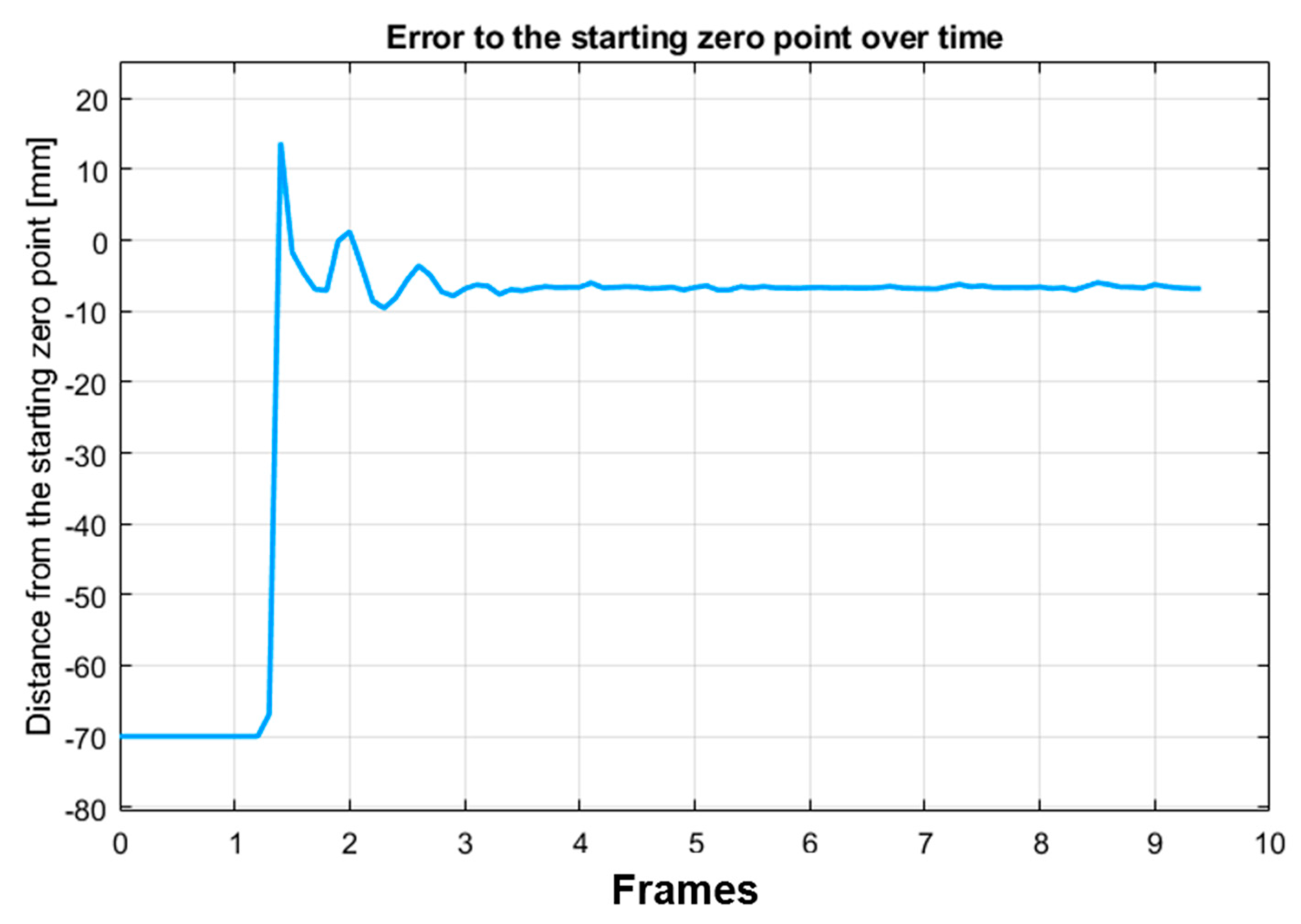
The error in control action represents the current ball distance from the starting zero point. As it is possible to see in
Figure 14, the ball wobbled before reaching an equilibrium position at around 11 mm from the zero point. This is the control result for a time gain of 0.09 for the derivative calculation.
If we reduced the time gain, using a gain value of 0.08, we reached better performance of the control action. In
Figure 15, we could not exactly reach the zero point on the error graph. We still had a little gap (~8 mm) between the zero (the starting zero point) and the real position reached at equilibrium.
Basically, the control has been done on position but using the velocity. We calculated the distance covered from the previous position: in this way, the new distance was computed from the absolute position and the starting zero point (the desired position). The result achieved was a very good result: reaching the balance, at a desired point, with a non-performant mechanical system (friction, light environment and table stability) and using a low-cost depth camera for the acquisition.
6. Conclusions
In this paper, we have shown it is possible to control a mechanical system employing an RGB-D vision device. We have implemented a methodology composed by two main procedures, both employing a vision device: one to detect a target object position combining color segmentation and a regression fitting procedure in the 3D space; another to measure the actuator displacement based on its shape and geometrical features. These two algorithms have been combined in a closed-loop control scheme. As a first application, we have proposed a tracking action of a target colored object by the linear actuator. As a second application, we have set up equipment to keep a ball in equilibrium on a slide moved by the actuator. Even in this case, the developed control model still employed the vision system as feedback, and it reconstructed the ball position starting from its velocity. The control strategy worked by introducing a basic prediction capability by measuring the position of the sphere through its velocity. It was possible to stop the ball around a desired position and maintain the ball at rest despite the low-cost equipment and a simple adopted benchmark. The advantage of using a vision system is the ability to directly observe the phenomenon to be controlled, also including the effects produced by mechanical limitations such as the delay of the actuation.
In a future perspective, such methodologies could be applied to more complicated mechanical systems to develop vision-based control strategies for industrial applications or for autonomous driving systems.

 ,
, 


