Advanced Strategy of Speed Predictive Control for Nonlinear Synchronous Reluctance Motors


 ,
,  ,
, 
Abstract
1. Introduction
2. Drive Model
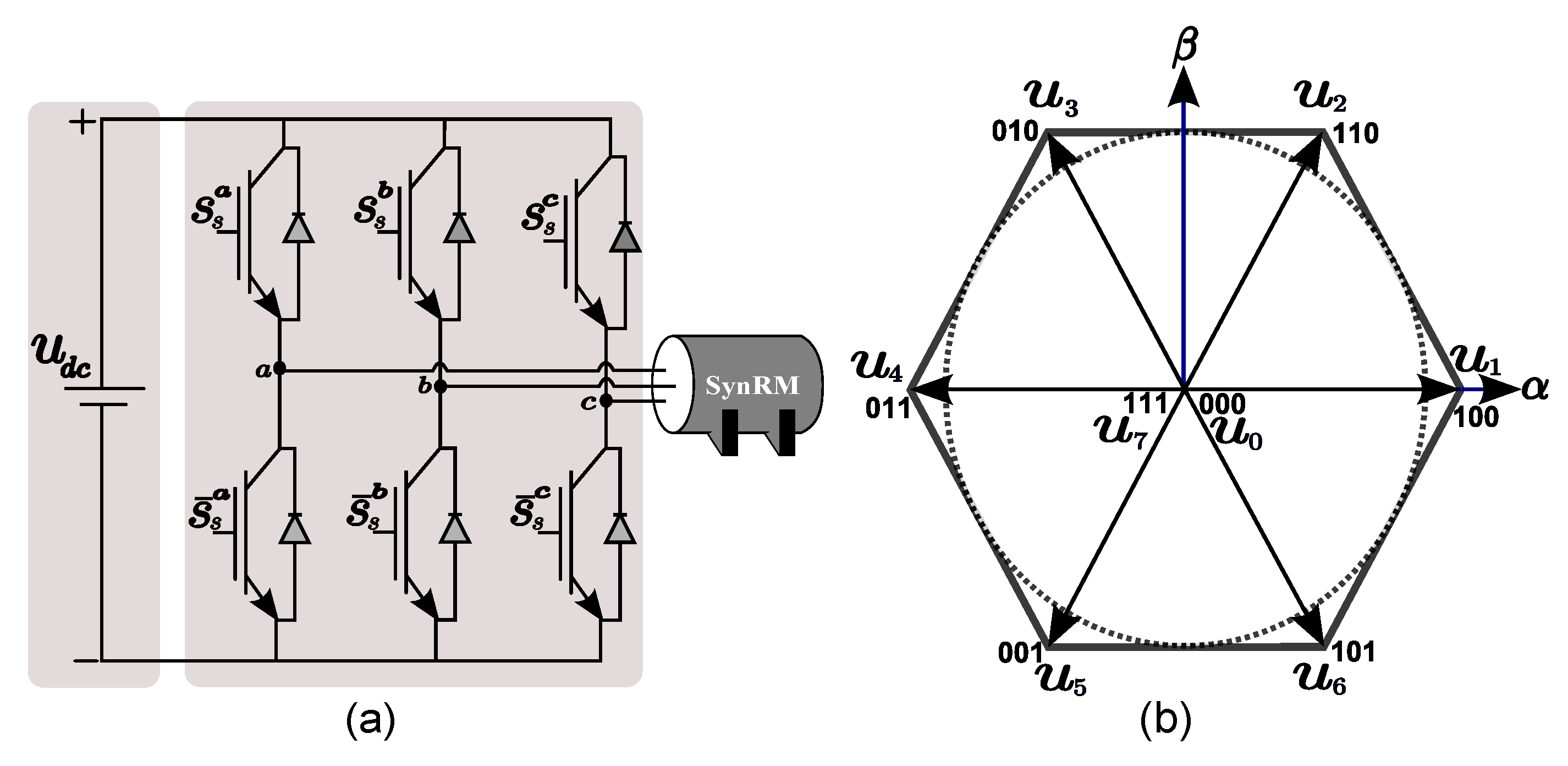
2.1. Inverter Model
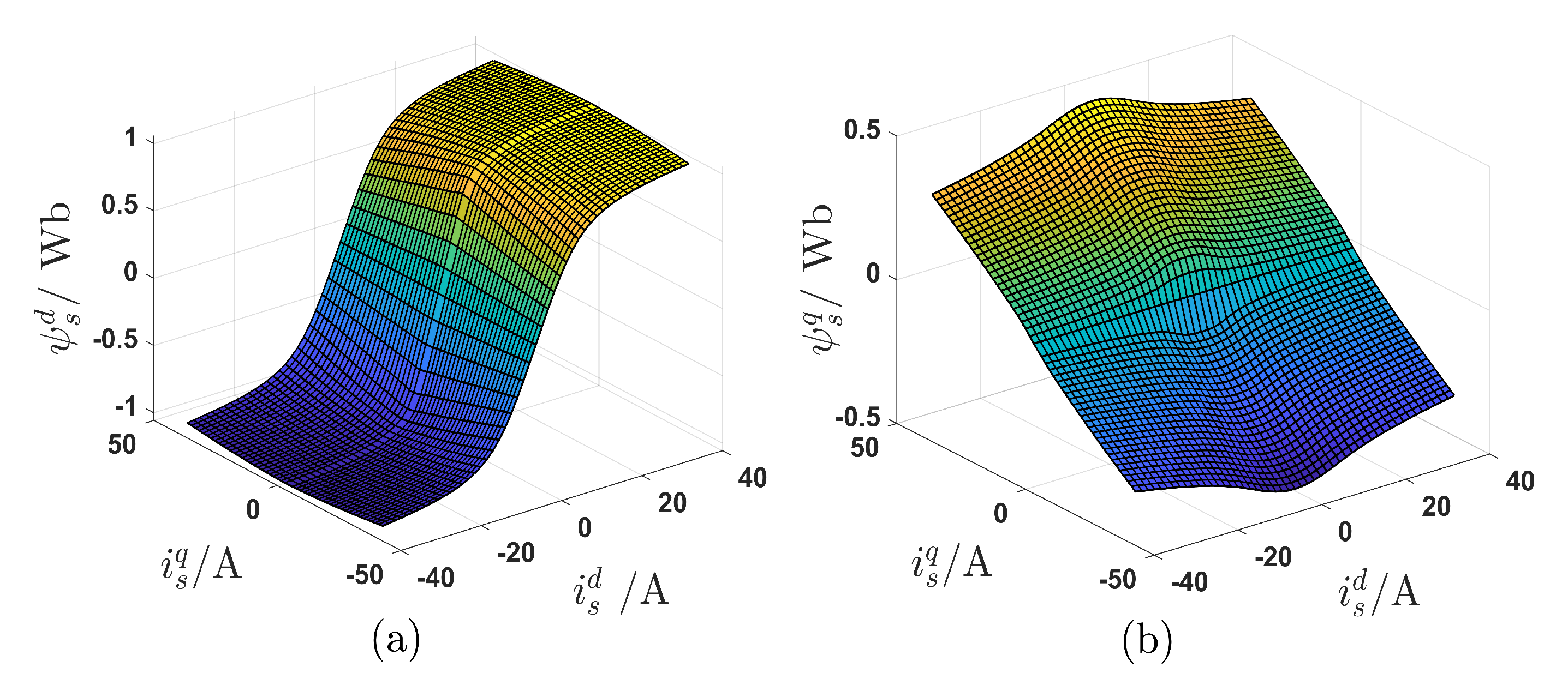
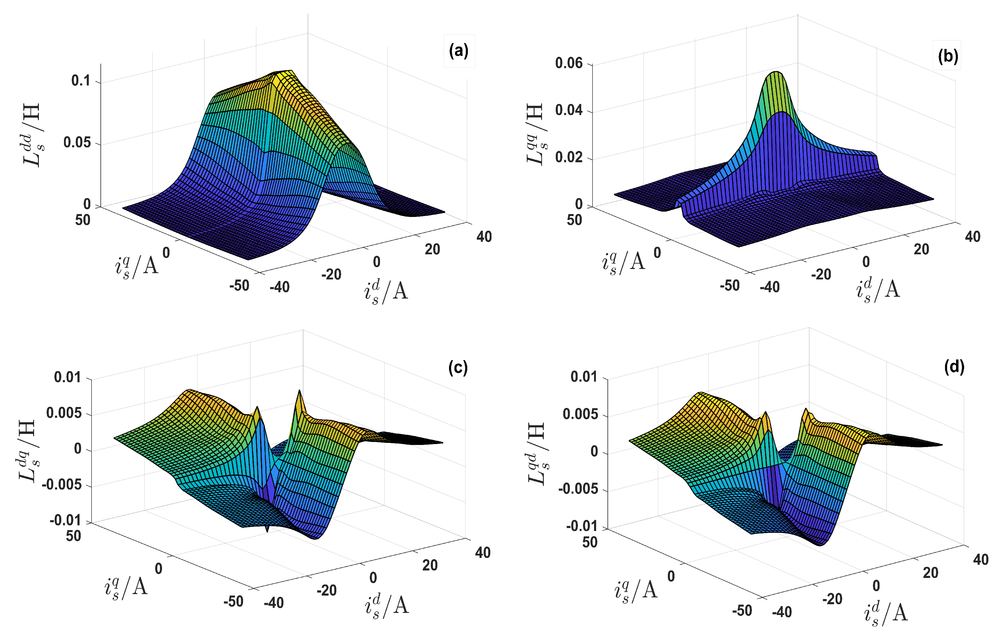
2.2. Synchronous Reluctance Motor Modeling
3. Control Strategies
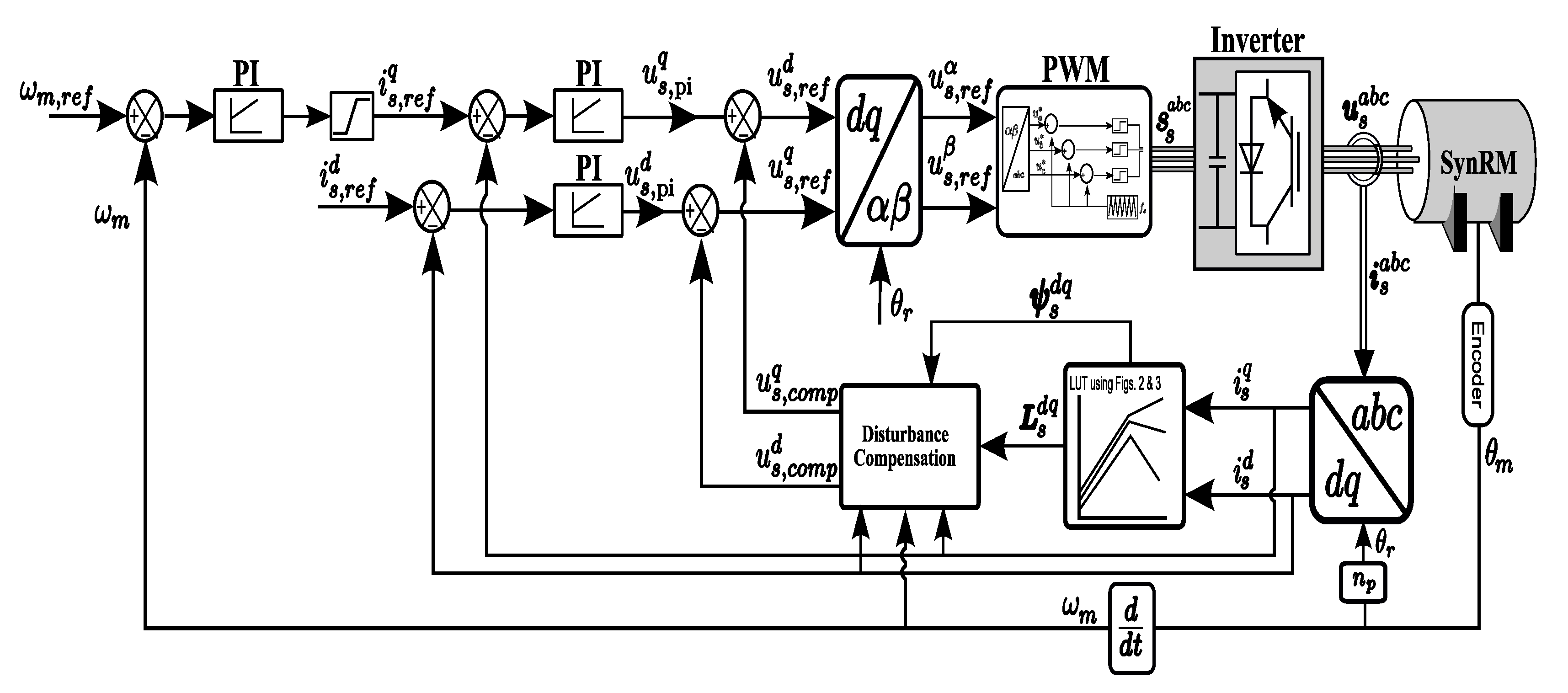
3.1. Field-Oriented Control Strategy
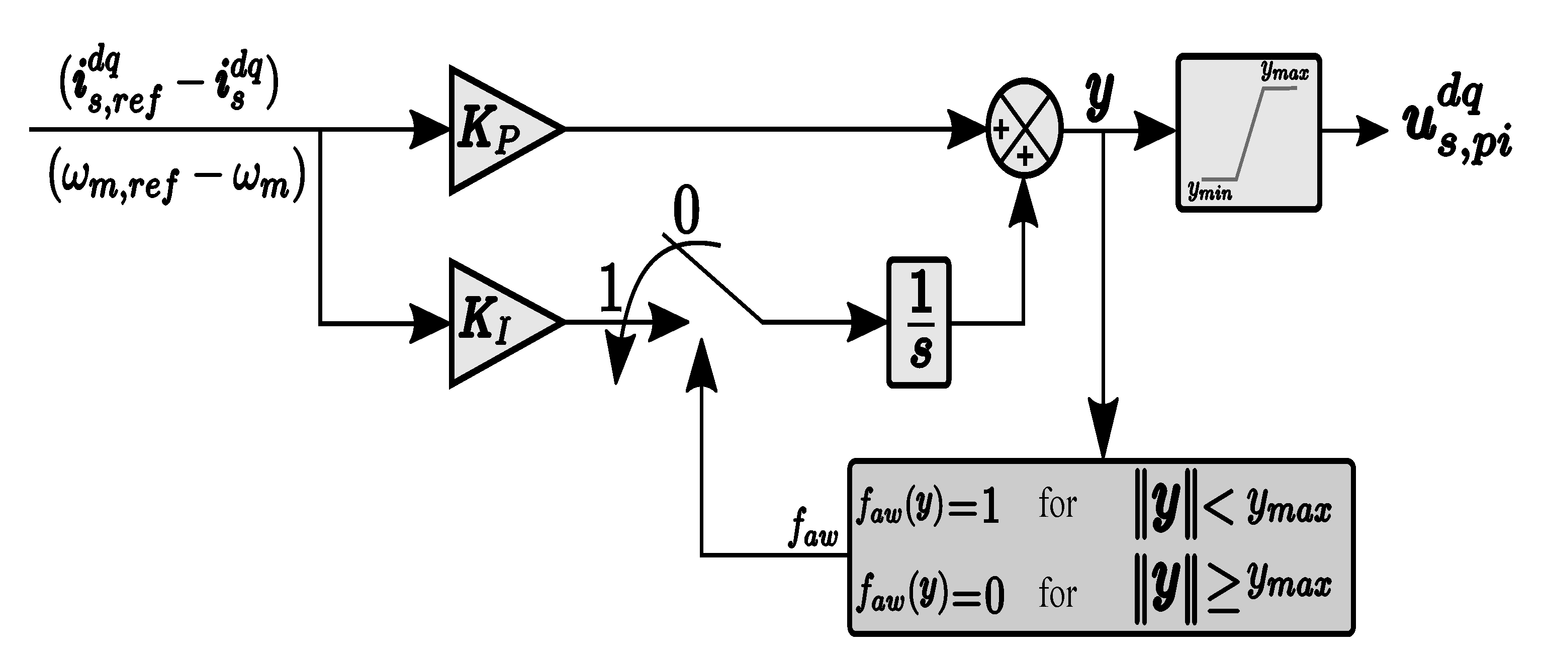
3.1.1. Anti-Windup Scheme
3.1.2. Field-Oriented Control of Nonlinear SynRM
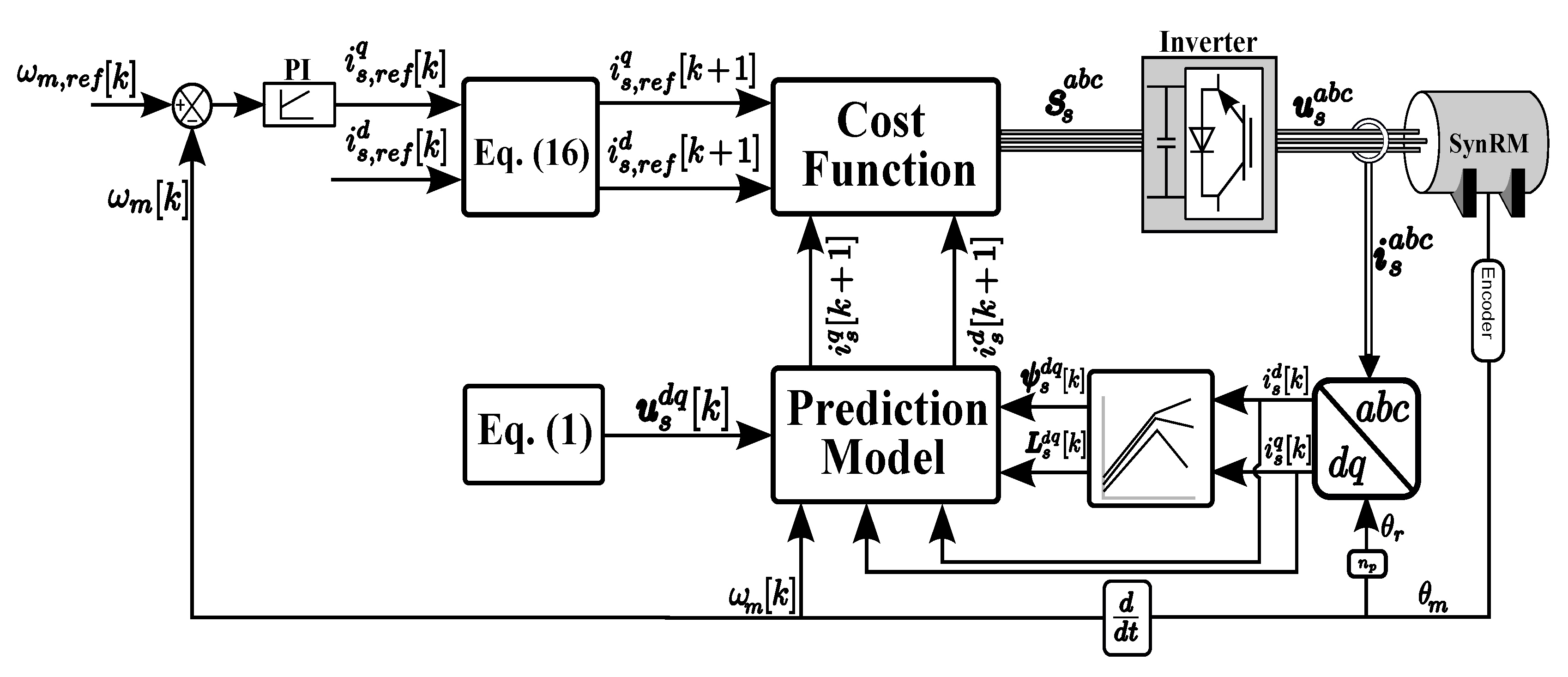
3.2. Current Predictive Control Strategy
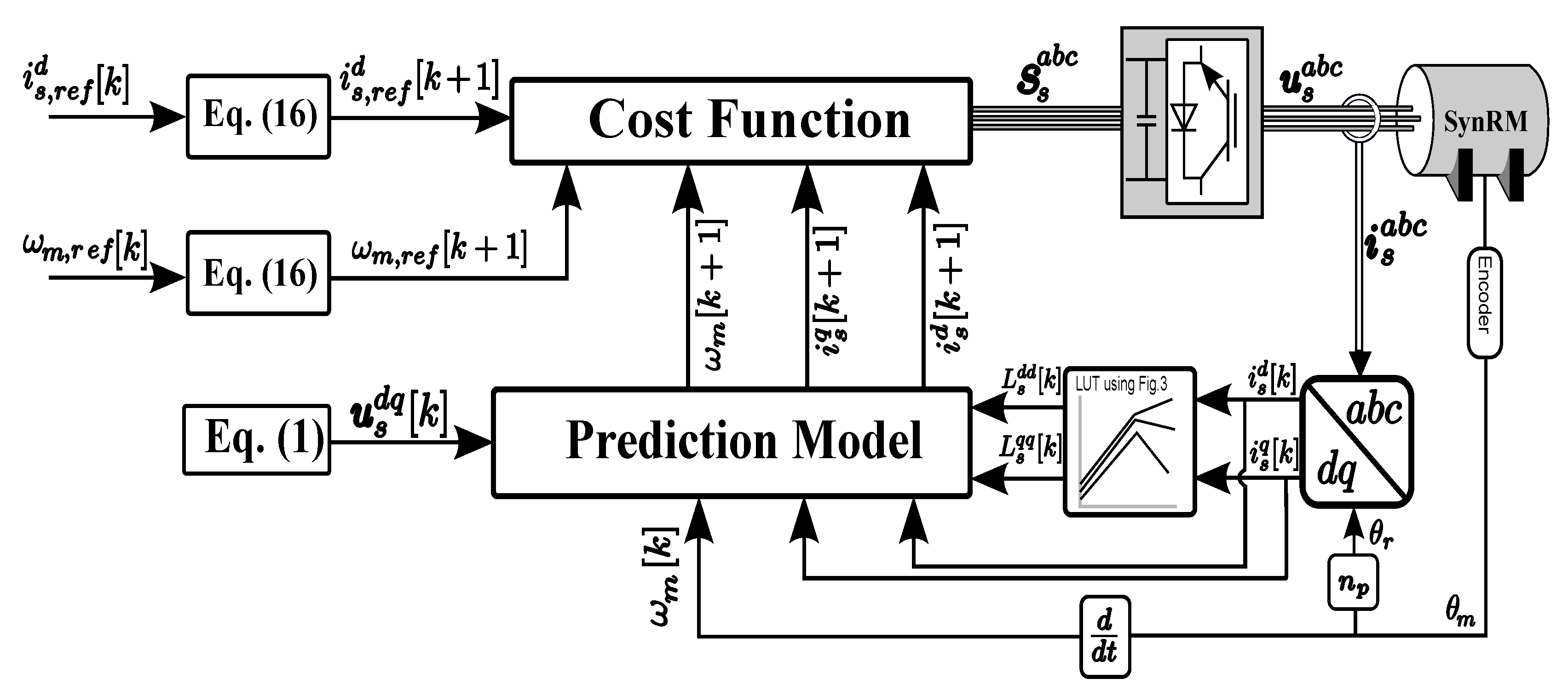
3.3. The Proposed Speed Predictive Control
| Algorithm 1 The proposed DSPC |
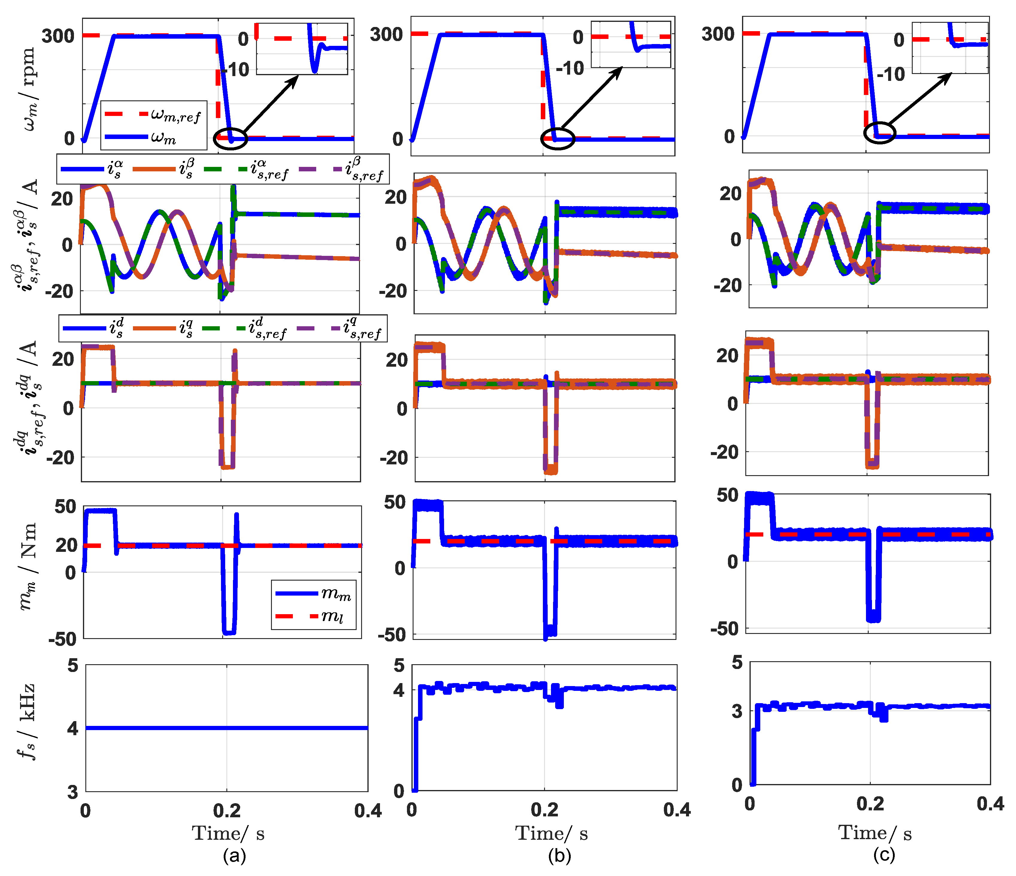
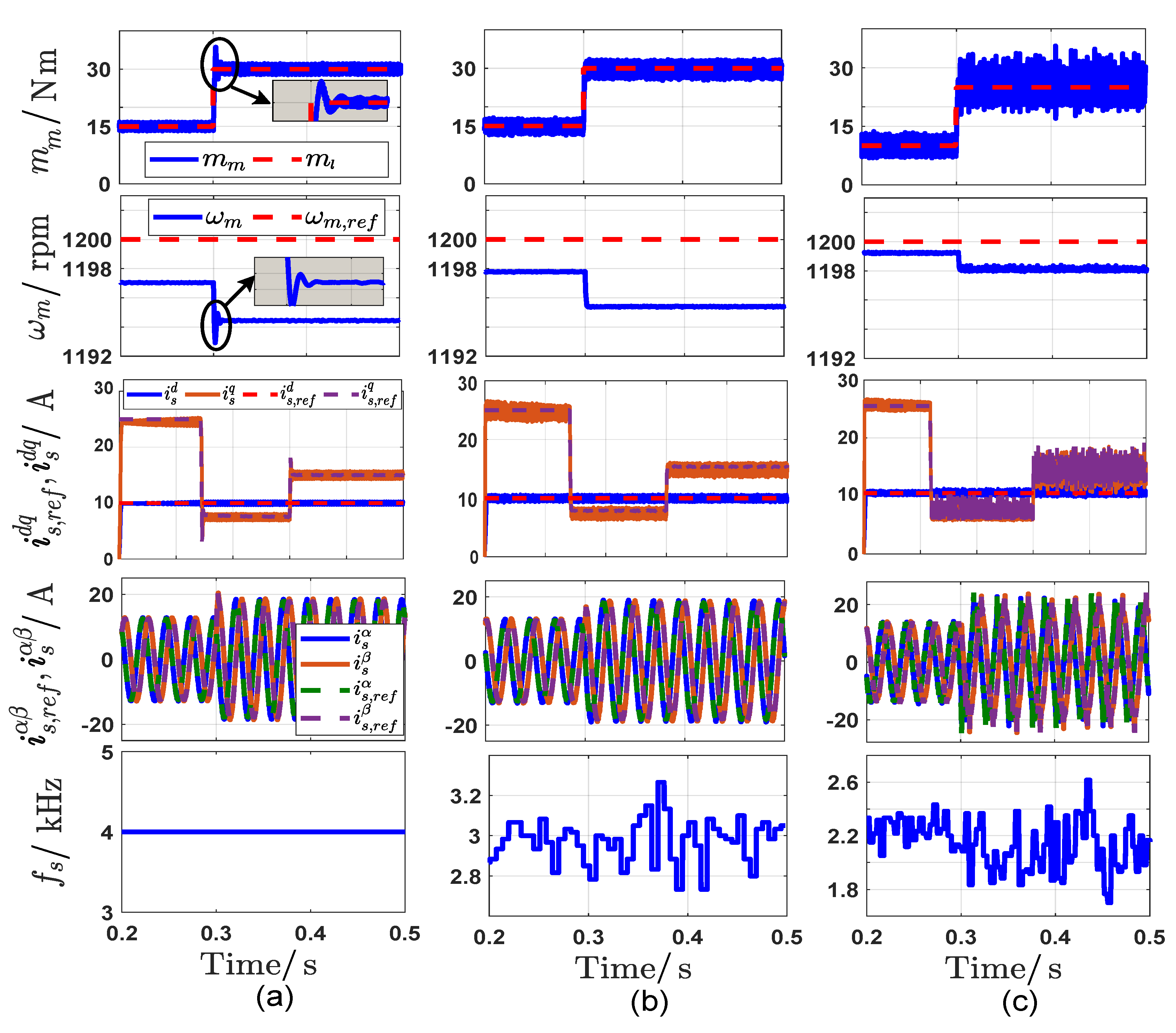
3.4. The Difference of Control Strategies
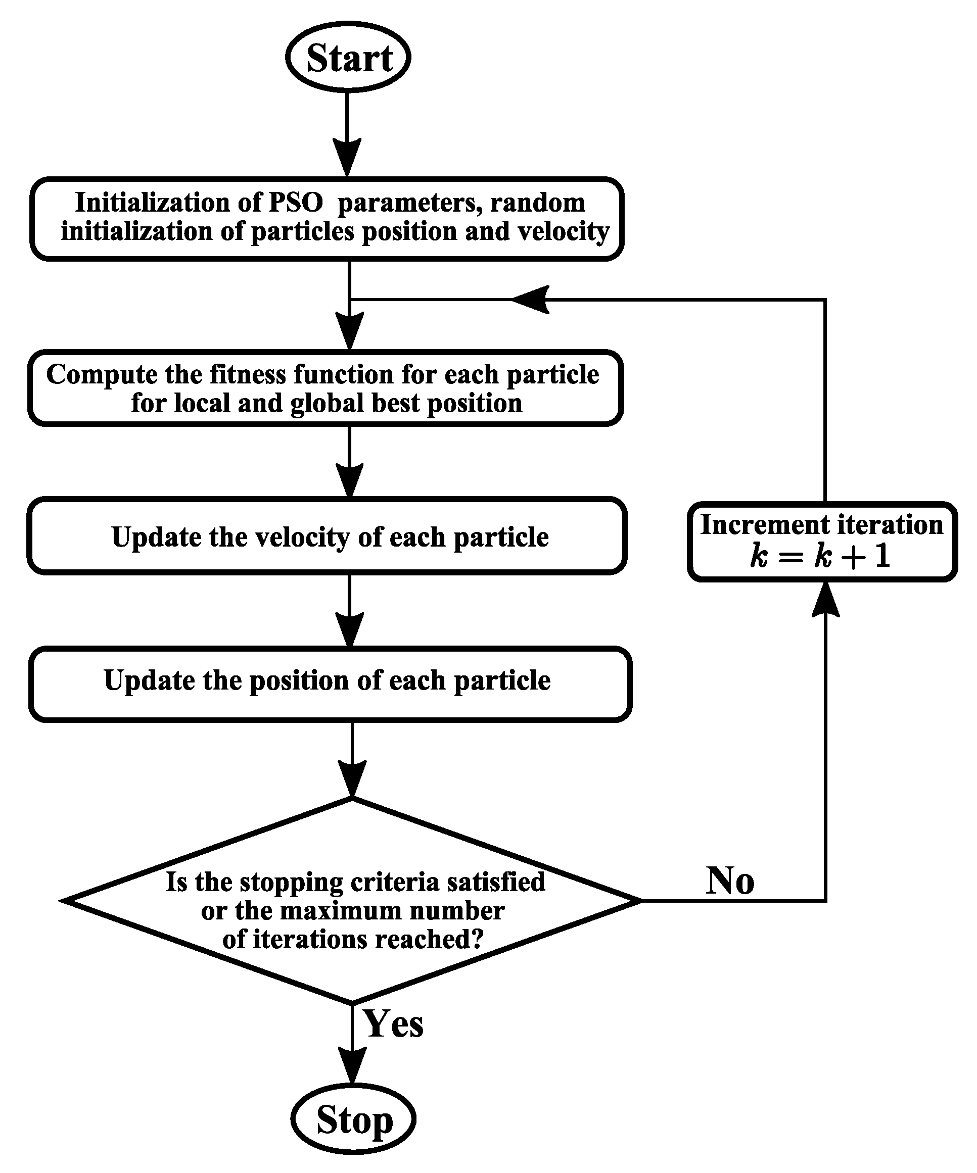
4. Particle Swarm Optimization
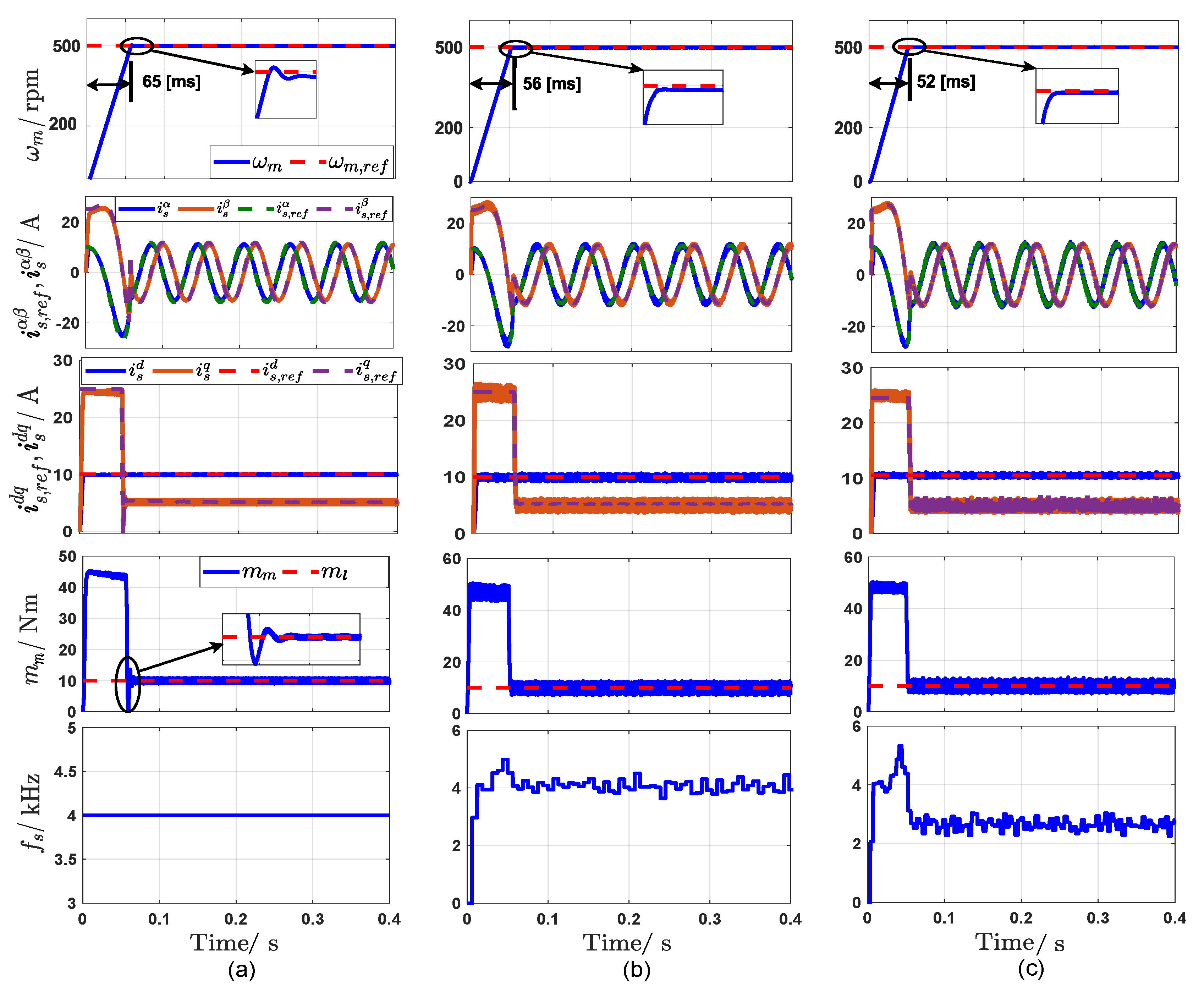
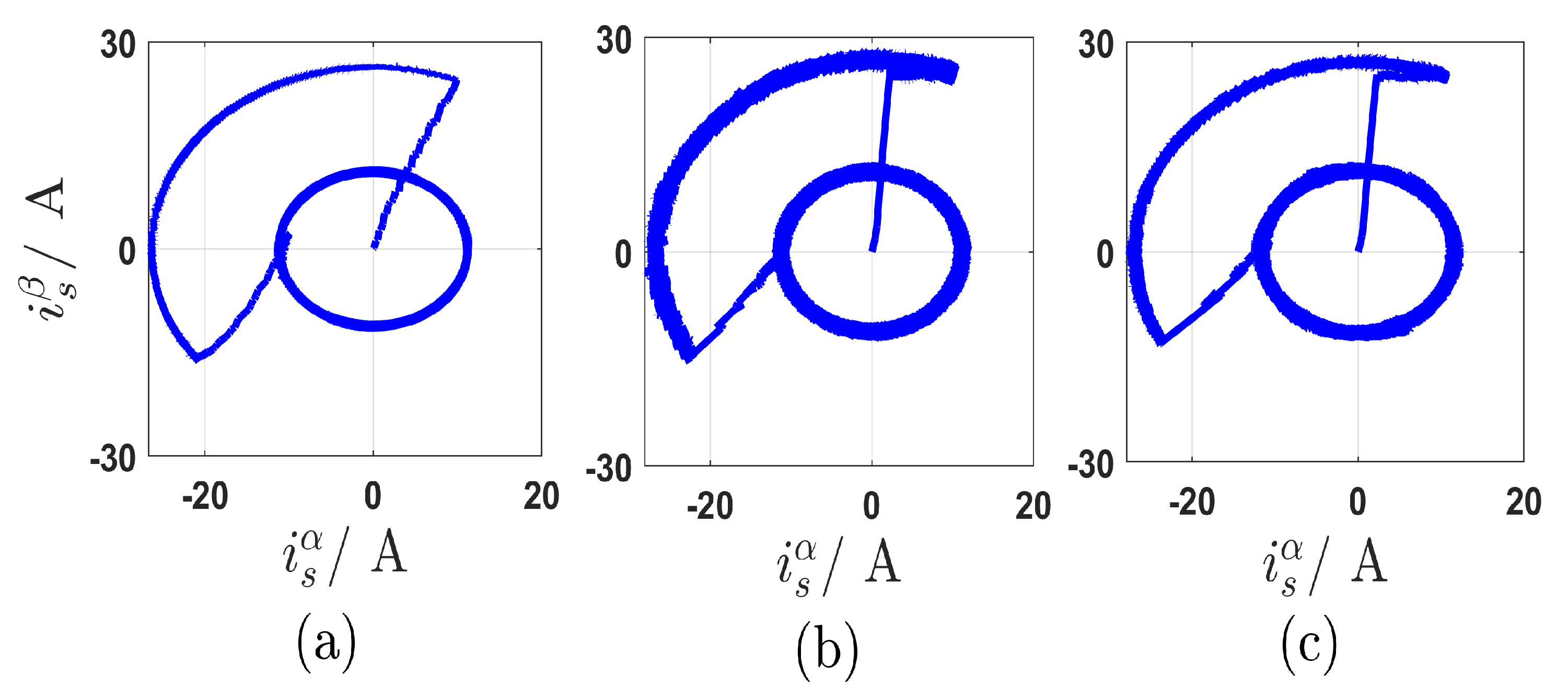
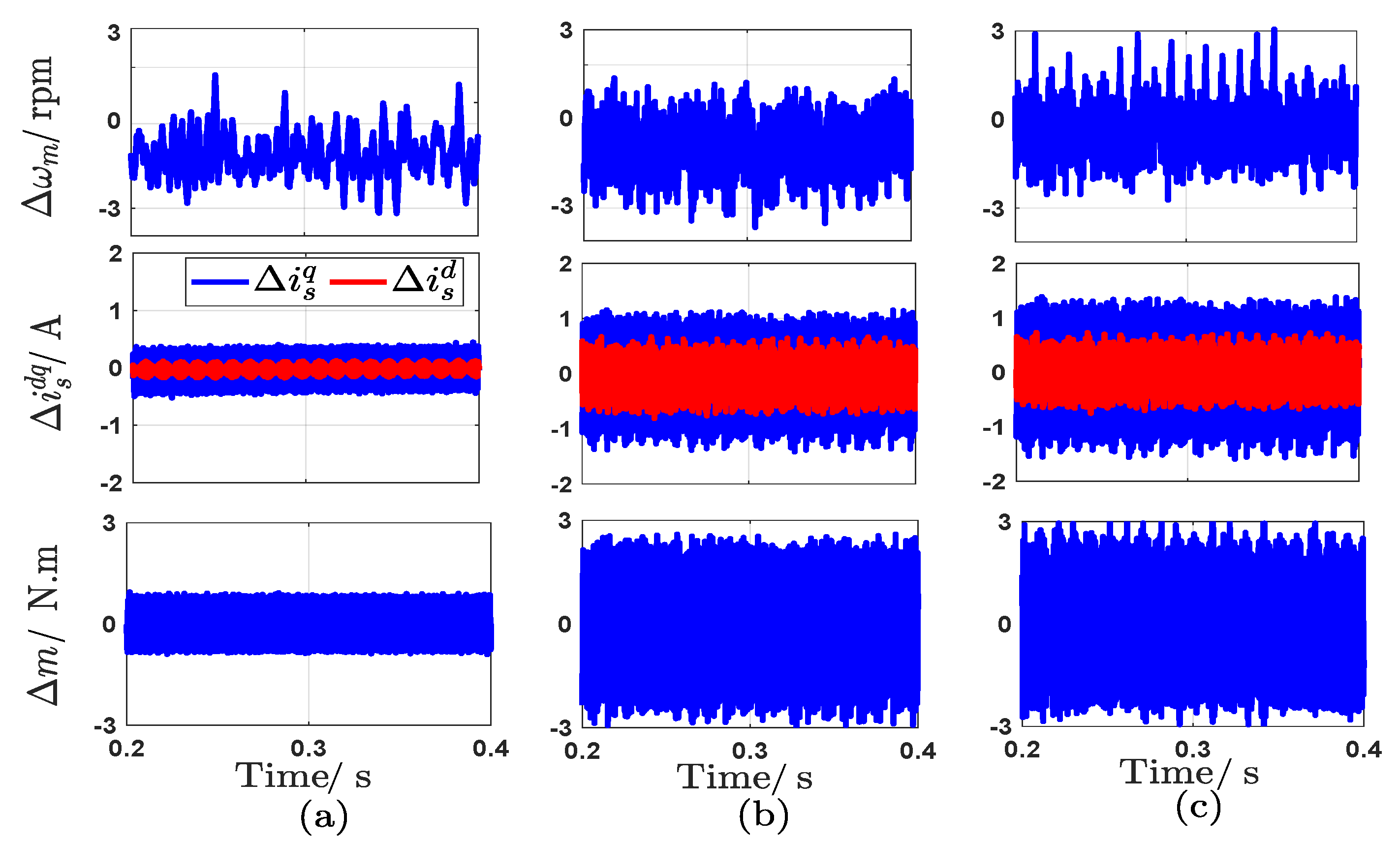
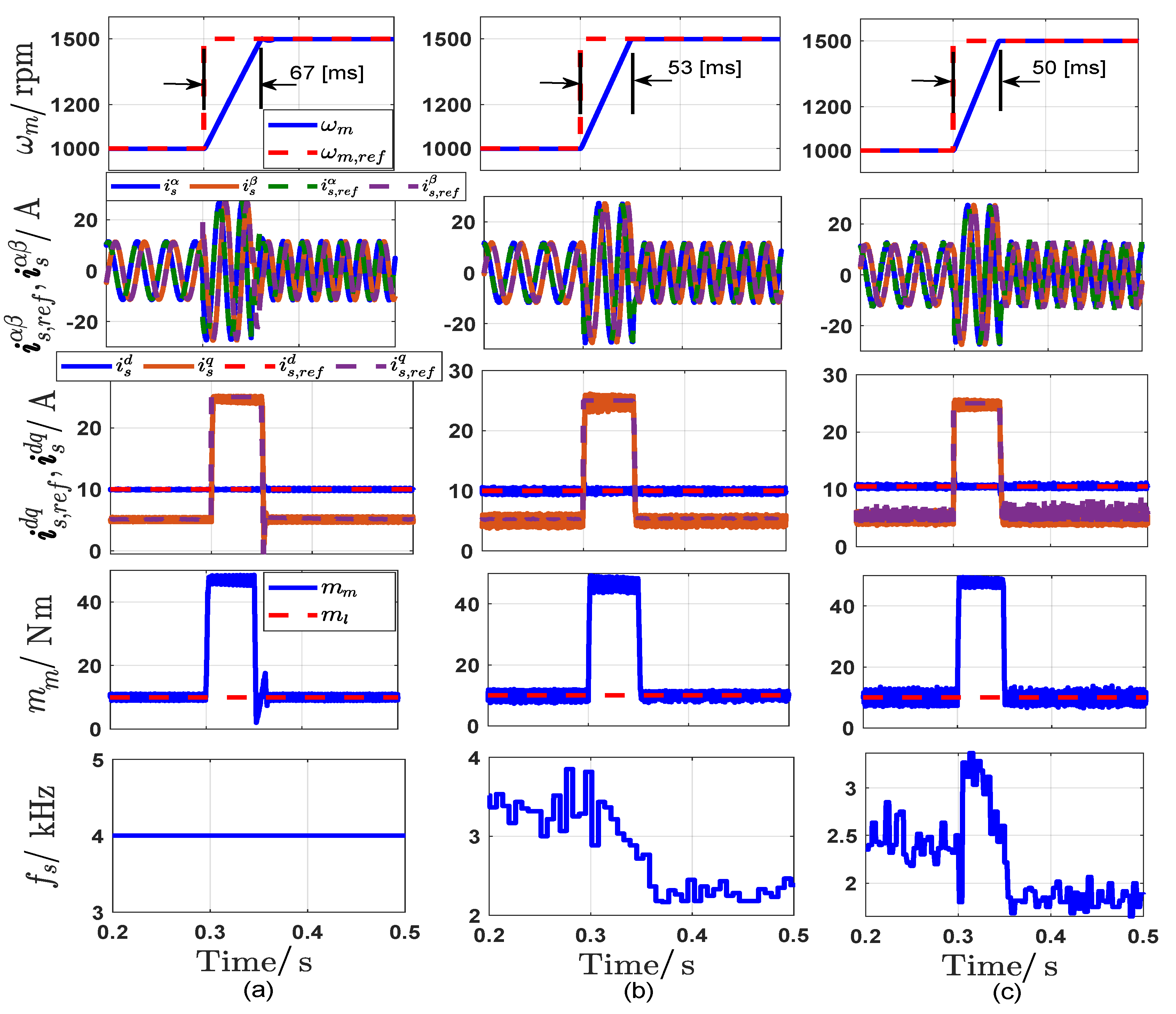
5. Simulation Results and Discussion
6. Conclusions
Author Contributions
Funding
Acknowledgments
Conflicts of Interest
Nomenclature
| Variables | |
| , | Stator voltages and currents in the rotating frame |
| , | Stator fluxes and inductances in the rotating frame |
| , | Stator resistance, rotor inertia, and viscous friction |
| , | Electrical position, electrical speed, and mechanical speed of the rotor () |
| Machine electromagnetic torque and load torque | |
| , | Pole pairs number, switching frequency, sample, and sampling time |
| Notation | |
| , , | Scalar, vector, and matrix, respectively |
References
- Wang, F.; Zhang, Z.; Mei, X.; Rodríguez, J.; Kennel, R. Advanced control strategies of induction machine: Field oriented control, direct torque control and model predictive control. Energies 2018, 11, 120. [Google Scholar] [CrossRef]
- Lin, C.K.; Lai, Y.S.; Yu, H.C. Improved model-free predictive current control for synchronous reluctance motor drives. IEEE Trans. Ind. Electron. 2016, 63, 3942–3953. [Google Scholar] [CrossRef]
- Farhan, A.; Abdelrahem, M.; Saleh, A.; Shaltout, A.; Kennel, R. Simplified Sensorless Current Predictive Control of Synchronous Reluctance Motor Using Online Parameter Estimation. Energies 2020, 13, 492. [Google Scholar] [CrossRef]
- Hackl, C.M.; Kamper, M.J.; Kullick, J.; Mitchell, J. Current control of reluctance synchronous machines with online adjustment of the controller parameters. In Proceedings of the 2016 IEEE 25th International Symposium on Industrial Electronics (ISIE), Santa Clara, CA, USA, 8–10 June 2016; IEEE: Piscataway, NJ, USA, 2016; pp. 153–160. [Google Scholar]
- Farhan, A.; Saleh, A.; Shaltout, A. High performance reluctance synchronous motor drive using field oriented control. In Proceedings of the 2013 5th International Conference on Modelling, Identification and Control (ICMIC), Cairo, Egypt, 31 August–2 September 2013; IEEE: Piscataway, NJ, USA, 2013; pp. 181–186. [Google Scholar]
- Lagerquist, R.; Boldea, I.; Miller, T.J. Sensorless-control of the synchronous reluctance motor. IEEE Trans. Ind. Appl. 1994, 30, 673–682. [Google Scholar] [CrossRef]
- Hackl, C.M. Non-Identifier Based Adaptive Control in Mechatronics: Theory and Application; Springer: Berlin/Heidelberg, Germany, 2017; Volume 466. [Google Scholar]
- Hackl, C.M.; Kamper, M.J.; Kullick, J.; Mitchell, J.; Nonlinear, P.I. Current control of reluctance synchronous machines. arXiv, 2015; arXiv:1512.09301. [Google Scholar]
- Hwang, S.H.; Kim, J.M.; Van Khang, H.; Ahn, J.W. Parameter identification of a synchronous reluctance motor by using a synchronous PI current regulator at a standstill. J. Power Electron. 2010, 10, 491–497. [Google Scholar] [CrossRef]
- Radimov, N.; Ben-Hail, N.; Rabinovici, R. Inductance measurements in switched reluctance machines. IEEE Trans. Magn. 2005, 41, 1296–1299. [Google Scholar] [CrossRef]
- Rafajdus, P.; Hrabovcova, V.; Lehocky, P.; Makys, P.; Holub, F. Effect of Saturation on Field Oriented Control of the New Designed Reluctance Synchronous Motor. Energies 2018, 11, 3223. [Google Scholar] [CrossRef]
- Arkadan, A.A.; Isaac, F.N.; Mohammed, O.A. Parameters evaluation of ALA synchronous reluctance motor drives. IEEE Trans. Magn. 2000, 36, 1950–1955. [Google Scholar] [CrossRef]
- Matsuo, T.; Lipo, T.A. Field oriented control of synchronous reluctance machine. In Proceedings of the IEEE Power Electronics Specialist Conference-PESC’93, Seattle, WA, USA, 20–24 June 1993; IEEE: Piscataway, NJ, USA, 1993; pp. 425–431. [Google Scholar]
- Ghaderi, A.; Hanamoto, T. Wide-speed-range sensorless vector control of synchronous reluctance motors based on extended programmable cascaded low-pass filters. IEEE Trans. Ind. Electron. 2010, 58, 2322–2333. [Google Scholar] [CrossRef]
- Zhang, Y.; Yang, H. Two-vector-based model predictive torque control without weighting factors for induction motor drives. IEEE Trans. Power Electron. 2015, 31, 1381–1390. [Google Scholar] [CrossRef]
- Lin, C.K.; Liu, T.H.; Fu, L.C.; Hsiao, C.F. Model-free predictive current control for interior permanent-magnet synchronous motor drives based on current difference detection technique. IEEE Trans. Ind. Electron. 2013, 61, 667–681. [Google Scholar] [CrossRef]
- Abdelrahem, M.; Hackl, C.M.; Kennel, R.; Rodriguez, J. Efficient direct-model predictive control with discrete-time integral action for PMSGs. IEEE Trans. Energy Convers. 2018, 34, 1063–1072. [Google Scholar] [CrossRef]
- Ahmed, A.A.; Koh, B.K.; Lee, Y.I. A comparison of finite control set and continuous control set model predictive control schemes for speed control of induction motors. IEEE Trans. Ind. Inform. 2017, 14, 1334–1346. [Google Scholar] [CrossRef]
- Gonçalves, P.F.; Cruz, S.M.; Mendes, A.M. Comparison of model predictive control strategies for six-phase permanent magnet synchronous machines. In Proceedings of the IECON 2018-44th Annual Conference of the IEEE Industrial Electronics Society, Washington, DC, USA, 21–23 October 2018; IEEE: Piscataway, NJ, USA, 2018; pp. 5801–5806. [Google Scholar]
- Gonçalves, P.; Cruz, S.; Mendes, A. Finite control set model predictive control of six-phase asymmetrical machines—An overview. Energies 2019, 12, 4693. [Google Scholar] [CrossRef]
- Abdelrahem, M.; Hackl, C.; Kennel, R.; Rodriguez, J. Sensorless predictive speed control of permanent-magnet synchronous generators in wind turbine applications. In PCIM Europe 2019, Proceedings of the International Exhibition and Conference for Power Electronics, Intelligent Motion, Renewable Energy and Energy Management, Nuremberg, Germany, 7–9 May 2019; VDE: Frankfurt, Germany, 2019; pp. 1–8. [Google Scholar]
- Morales-Caporal, R.; Pacas, M. A predictive torque control for the synchronous reluctance machine taking into account the magnetic cross saturation. IEEE Trans. Ind. Electron. 2007, 54, 1161–1167. [Google Scholar] [CrossRef]
- Farhan, A.; Saleh, A.; Shaltout, A.; Kennel, R. Encoderless Finite Control Set Predictive Current Control of Synchronous Reluctance Motor. In Proceedings of the 2019 21st International Middle East Power Systems Conference (MEPCON), Cairo, Egypt, 17–19 December 2019; IEEE: Piscataway, NJ, USA, 2019; pp. 692–697. [Google Scholar]
- Hadla, H.; Cruz, S. Predictive stator flux and load angle control of synchronous reluctance motor drives operating in a wide speed range. IEEE Trans. Ind. Electron. 2017, 64, 6950–6959. [Google Scholar] [CrossRef]
- Hadla, H.; Cruz, S. Active flux based finite control set model predictive control of synchronous reluctance motor drives. In Proceedings of the 2016 18th European Conference on Power Electronics and Applications (EPE’16 ECCE Europe), Karlsruhe, Germany, 5–9 September 2016; IEEE: Piscataway, NJ, USA, 2019; pp. 1–10. [Google Scholar]
- Preindl, M.; Bolognani, S. Model predictive direct speed control with finite control set of PMSM drive systems. IEEE Trans. Power Electron. 2012, 28, 1007–1015. [Google Scholar] [CrossRef]
- Kakosimos, P.; Abu-Rub, H. Predictive speed control with short prediction horizon for permanent magnet synchronous motor drives. IEEE Trans. Power Electron. 2017, 33, 2740–2750. [Google Scholar] [CrossRef]
- Liu, T.H.; Haslim, H.S.; Tseng, S.K. Predictive controller design for a high-frequency injection sensorless synchronous reluctance drive system. IET Electr. Power Appl. 2017, 11, 902–910. [Google Scholar] [CrossRef]
- Hackl, C.M.; Larcher, F.; Dötlinger, A.; Kennel, R.M. Is multiple-objective model-predictive control “optimal”? In Proceedings of the 2013 IEEE International Symposium on Sensorless Control for Electrical Drives and Predictive Control of Electrical Drives and Power Electronics (SLED/PRECEDE), Munich, Germany, 17–19 October 2013; IEEE: Piscataway, NJ, USA, 2013; pp. 1–8. [Google Scholar]
- Bolognani, S.; Tubiana, L.; Zigliotto, M. Extended Kalman filter tuning in sensorless PMSM drives. IEEE Trans. Ind. Appl. 2003, 39, 1741–1747. [Google Scholar] [CrossRef]
- Solihin, M.I.; Tack, L.F.; Kean, M.L. Tuning of PID controller using particle swarm optimization (PSO). Proceeding of the International Conference on Advanced Science, Engineering and Information Technology, Bangi, Malaysia, 14–15 January 2011; Volume 1, pp. 458–461. [Google Scholar]
- Farhan, A.; Saleh, A.; Abdelrahem, M.; Kennel, R.; Shaltout, A. High-Precision Sensorless Predictive Control of Salient-Pole Permanent Magnet Synchronous Motor based-on Extended Kalman Filter. In Proceedings of the 2019 21st International Middle East Power Systems Conference (MEPCON), Cairo, Egypt, 17–19 December 2019; IEEE: Piscataway, NJ, USA, 2019; pp. 226–231. [Google Scholar]
- Del Valle, Y.; Venayagamoorthy, G.K.; Mohagheghi, S.; Hernez, J.C.; Harley, R.G. Particle swarm optimization: Basic concepts, variants and applications in power systems. IEEE Trans. Evol. Comput. 2008, 12, 171–195. [Google Scholar] [CrossRef]
- Calvini, M.; Carpita, M.; Formentini, A.; Marchesoni, M. PSO-based self-commissioning of electrical motor drives. IEEE Trans. Ind. Electron. 2014, 62, 768–776. [Google Scholar] [CrossRef]
- Ghoshal, A.; John, V. Anti-Windup Schemes for Proportional Integral and Proportional Resonant Controller. Proceedings of National Power Electronics Conference, Roorkee, India, 10–13 June 2010; pp. 1–6. [Google Scholar]
- Eldeeb, H.; Hackl, C.M.; Horlbeck, L.; Kullick, J. A unified theory for optimal feedforward torque control of anisotropic synchronous machines. Int. J. Control 2018, 91, 2273–2302. [Google Scholar] [CrossRef]
- Garcia, C.; Silva, C.; Rodriguez, J.; Zanchetta, P. Cascaded model predictive speed control of a permanent magnet synchronous machine. In Proceedings of the IECON 2016-42nd Annual Conference of the IEEE Industrial Electronics Society, Florence, Italy, 23–26 October 2016; IEEE: Piscataway, NJ, USA, 2016; pp. 2714–2718. [Google Scholar]
- Maciejowski, J.M.; PRedictive Control: With Constraints. Pearson Education. 2002. Available online: https://onlinelibrary.wiley.com/doi/abs/10.1002/acs.736 (accessed on 15 June 2020).


| FOC | CPC | SPC | |
|---|---|---|---|
| Number of Parameters to tune | 6 | 2 | 2 |
| Number of External PI controllers | 1 | 1 | 0 |
| Number of Inner PI controllers | 2 | 0 | 0 |
| Pulse-width modulation | Yes | No | No |
| Coordinate Transformation | Yes | Yes | Yes |
| System Constraints | Difficult | Easy | Easy |
| Conceptual Complication | Low | Low | Low |
| Description | Nomenclature/Values/Unites |
|---|---|
| SynRM | kW, Ω, , as in Figure 2 and Figure 3 |
| A, rpm, rad/s, | |
| V ( Hz) | |
| Mechanic | kgm2, B = 0 |
| VSI | V |
| FOC | PI speed controller factors , |
| PI current controller factors , , | |
| Simulation step = 1 | |
| CPC | PI speed controller factors , = 40 , |
| Simulation step = 1 | |
| SPC | Weighting factors , = 40 , Simulation step = 1 |
| FOC | CPC | SPC | |
|---|---|---|---|
| Dynamic response | slow | fast | faster |
| Overshoot ratio | small | smaller | zero |
| Average SSE | low | low | lower |
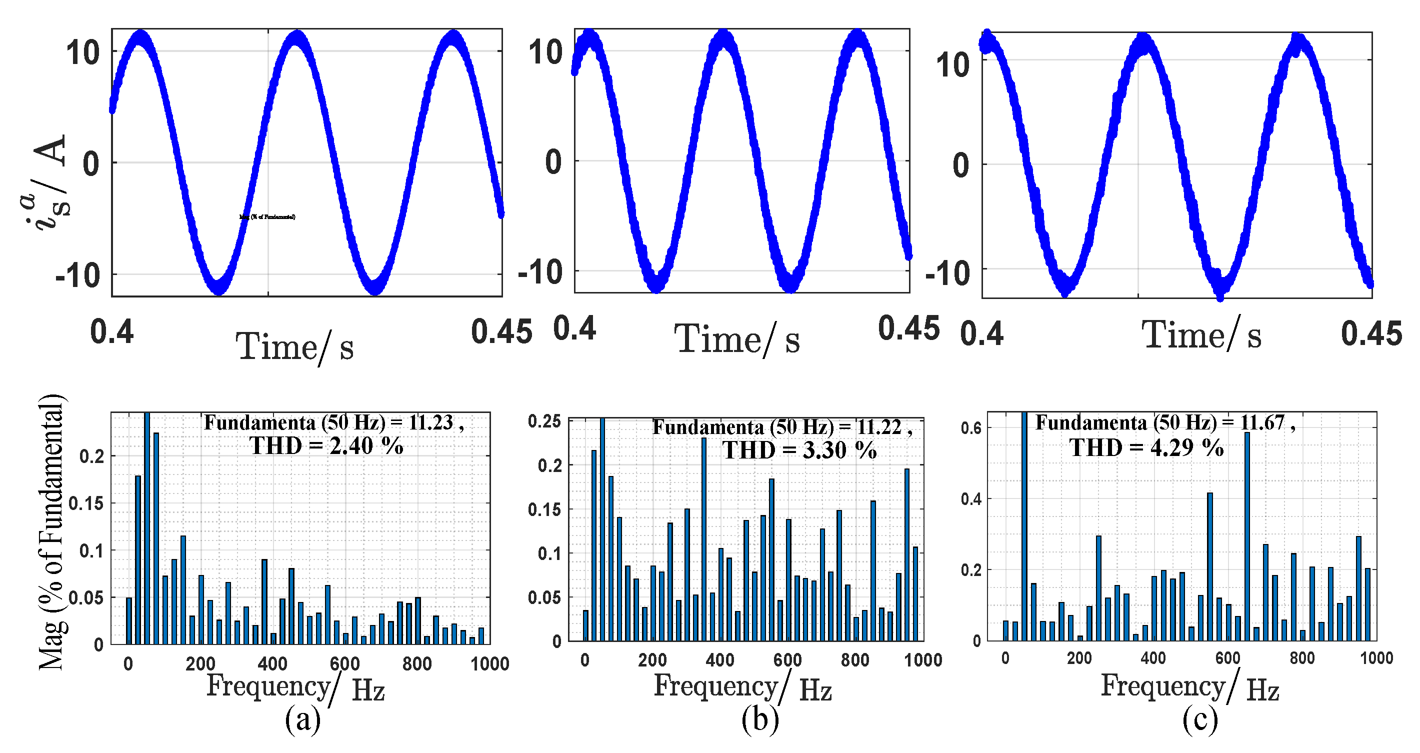
| Current THD | |||
| Torque ripples | low | some | more |
| Tracking error | low | low | low |
| Switching frequency | constant | variable | variable |
© 2020 by the authors. Licensee MDPI, Basel, Switzerland. This article is an open access article distributed under the terms and conditions of the Creative Commons Attribution (CC BY) license (http://creativecommons.org/licenses/by/4.0/).
Share and Cite
Farhan, A.; Abdelrahem, M.; Hackl, C.M.; Kennel, R.; Shaltout, A.; Saleh, A. Advanced Strategy of Speed Predictive Control for Nonlinear Synchronous Reluctance Motors. Machines 2020, 8, 44. https://doi.org/10.3390/machines8030044
Farhan A, Abdelrahem M, Hackl CM, Kennel R, Shaltout A, Saleh A. Advanced Strategy of Speed Predictive Control for Nonlinear Synchronous Reluctance Motors. Machines. 2020; 8(3):44. https://doi.org/10.3390/machines8030044
Chicago/Turabian StyleFarhan, Ahmed, Mohamed Abdelrahem, Christoph M. Hackl, Ralph Kennel, Adel Shaltout, and Amr Saleh. 2020. "Advanced Strategy of Speed Predictive Control for Nonlinear Synchronous Reluctance Motors" Machines 8, no. 3: 44. https://doi.org/10.3390/machines8030044
APA StyleFarhan, A., Abdelrahem, M., Hackl, C. M., Kennel, R., Shaltout, A., & Saleh, A. (2020). Advanced Strategy of Speed Predictive Control for Nonlinear Synchronous Reluctance Motors. Machines, 8(3), 44. https://doi.org/10.3390/machines8030044