Abstract
The advanced steel grades and high productivity requirements in the modern steel industry subject production machines to increased mechanical stresses, which inflicts losses. Novel data-oriented solutions to the monitoring of machines have a pivotal role in loss prevention, but the industrial data with high sampling rates, noise, and dimensions bring challenges there. This study proposes a new monitoring approach for roller levelers based on vibration measurements and regression models for estimating steel strip properties including yield strength, width, and thickness. The regression residuals are monitored based on moving mean and range charts, which reveal changes from the expected normal operation. A high-dimensional feature set of 144,000 statistical features was studied with various feature selection methods, including filters and wrappers. Multiple linear regression and generalized regression neural network were applied in modeling. The approach was validated using data from an industrial roller leveler processing steel strips with diverse properties. The results reveal that the accurate prediction of the strip thickness from the strip properties is possible and multiple linear regression was generally the superior model therein. Additional simulations indicated that the control charts can detect deviant operation. Supplemental information about the momentary operation of the machine would improve the approach.
1. Introduction
Modern day industry witnesses both the advantages and challenges arising from the extensive amount of continuously streaming data enabled by the contemporary Information and Communications Technology (ICT) and initiatives, such as “Industrie 4.0” and “Made in China 2025.” The key objectives in such initiatives include reaching maximal uptime throughout the production chain and increasing productivity while reducing the production cost [1]. One of the important approaches supporting such objectives is the Condition-Based Maintenance (CBM), where the degradation process of the system is monitored and perhaps even predicted before the breakdown [2]. CBM benefits from the information contained in the abundant data provided by numerous sensors and other data sources, but on the other hand, the selection of the useful data remains a challenge. The large data sets are subjected to substantial selection bias and measurement errors, which have an enormous influence on the decisions made based on the data [3]. In the fields of CBM and monitoring, a significant part of development should be directed to data pre-processing including data selection and preparation, feature extraction and selection, and model selection in order to avoid the “garbage in—garbage out” scenarios.
This study focuses on the condition monitoring of roller levelers which are used in steel factories to straighten steel strips after final rolling, heat treatment or cooling operations. These machines are exposed to high mechanical stresses [4] due to the advanced steel grades processed [5] and the increasing demands for productivity. Therefore, the monitoring of such machines becomes increasingly important, but relatively few studies deal with the condition monitoring of such machines [6]. Instead, most of the studies are concerned with process simulations, parameter analysis, and the behavior of material in the leveling process [7,8].
Vibration analysis was selected as the technique to be utilized in the monitoring in this study, because acceleration signals are sensitive to the varying forces inflicted on the machine and have proven useful in various applications [9]. Other commonly used techniques in industrial monitoring include acoustic emission, oil debris, ultrasound, and temperature monitoring [10]. The acoustic emission is often used for similar tasks as the vibration, but it has practical challenges resulting from the lack of established calibration methods [11,12], the requirement of direct signal path through solid material [12], and high sampling rates [13]. In addition, the reliability of acoustic measurements [14,15] may be compromised due to the extensive background noises in factories. For these reasons, the well-established vibration techniques appear more appropriate for many industrial applications. Instead of analyzing the individual samples in the signals, vibration signals are commonly monitored based on features and signal transformations [16,17]. However, the direct use of an autoregressive model [18] and deep learning algorithms [19] on the signals have been proposed as well. Due to the noisy industrial environment, the conventional feature engineering approach was considered more appropriate for the approach studied here. In the case of roller levelers, there is, however, limited information on which features are useful for the monitoring of structural vibration when the monitoring is not targeted at a specific component, such as the bearing, shaft, or gear. Correlations between a few vibration features and machine parameters were studied in [6], but it was not shown how this information could be used in monitoring.
To get insight into the operation of the machine, an appropriate solution could be the generation of a large set of features and transformations from the vibration signals, i.e., the production of a high-dimensional data set for data mining. In order to identify the characteristics or the typical operation of the machine, the use of statistical features provides a practical solution. In this study, features such as the generalized norms [20], other features derived from them, and percentiles in short time windows are used. Such features have proven useful in previous applications in the monitoring of machine vibration [4,9,21]. Before extracting these time domain features, the complete signals are also filtered by using various frequency bands with different sizes. Furthermore, the amplitudes of individual frequency components are computed, and statistical features are extracted from them in the successive time windows. The use of narrow frequency bands and individual frequency components could reveal effects masked behind other full or wide bandwidth effects and disturbances, which can be intensive in industrial surroundings. The flowchart for system identification in Figure 1 illustrates how the signal filtering and feature generation phases relate to the overall data mining procedure applied.
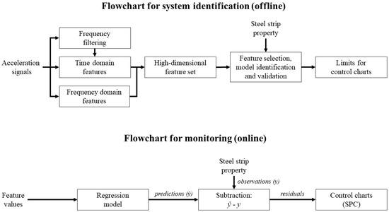
Figure 1.
Flowcharts depicting the system identification and online monitoring procedures of the proposed approach to roller leveler monitoring.
To make the application of a high-dimensional feature set practical, efficient feature selection algorithms are required. With such algorithms, the irrelevant and redundant features are removed, and the predictive qualities and comprehensibility of the selected feature set are improved. A multitude of approaches has been proposed for the computational feature selection [22]. These solutions are traditionally categorized as filters, wrappers, and embedded approaches [23]. The significance of selecting the right solution is pronounced with high-dimensional data, where the building of a global model with a complete set of features is not practical. In such circumstances, many classical approaches such as the least squares linear regression [24] or genetic algorithms [25] perform unfavorably due to the bias-variance trade-off and overfitting. Many of the methods try to find a good set of variables rather than the optimal set [25], which is also the expected end-result in the case of high-dimensional data sets. To tackle the problems of high-dimensionality, different solutions have been introduced, which include narrowing down the search space and the use of simple methods with low computation costs [26]. These principles are also followed in this study: Two relatively simple wrapper approaches and the combination of filters and exhaustive search are tested. The wrappers include the sequential forward selection [27] and the floating search algorithm proposed in [28]. To narrow down the search space, several information-theoretic filters [29] were first applied to generate small feature subsets. The exhaustive search was then applied in the modeling stage to find the optimal feature combination from the small subsets.
Numerous data-driven algorithms have been introduced to the condition monitoring of machines [30]. Quite common targets of application include the automated diagnosis of bearing faults [31] or gear and shaft damage [32]. Many of these approaches are based on the principle of supervised classification, which uses the presumption that all the monitored machine states can be trained to the classifier, which then gives a categorical (qualitative) representation of the machine condition. Alternatively, regression models can be used to estimate quantitative responses, such as the relative stress level [4] or other health indicators [33] from the monitored system. However, the solutions where the signal features are combined with the processed materials such as the steel strips in roller levelers, as shown in Figure 1, are rare [4]. The machine vibrations are associated with the processed materials, operational parameters, and external disturbances, which should be considered, because they affect the success of diagnosis [21] and prognosis [34]. The changes of operational parameters and operating states in industrial applications make the direct monitoring of single features challenging. Regression models are practical for combining the feature values with each operating state and for identifying the typical values in each state. In addition, the features together provide information that individual features cannot provide, which eventually may increase the modeling accuracy.
The previous approaches to the regression-based estimation of steel properties in steel forming include yield strength and tensile strength prediction [35] and hardness prediction [36] based on steel composition and other processing parameters. Additionally, process data have been used to predict processing parameters, such as force, torque and slab temperature in a rolling process by using genetic programming [37]. Then again, the modeling applications in roller leveling mostly focus on the analytical modeling of material behavior [8,38] or the leveling process [39,40,41]. Such approaches do not focus on the vibrations in the process. However, analytical models and vibration measurements were used in [42,43] to study the polygonal wear on work rolls in a hot leveler. In a recent study [4], the relative stress inflicted on a roller leveler was estimated based on vibration measurements.
The reported research on how the structural vibrations during leveling could be used to monitor the process is incomplete and rare. Therefore, this study proposes a data-driven approach to the identification of typical vibrations during the leveling process, which is illustrated in Figure 1. This approach can be used (1) in the online estimation of the strip properties based on regression models, and (2) in the detection of deviant operation based on Statistical Process Control (SPC) charts for the regression residuals. Although the residuals are monitored based on the strip properties as depicted in Figure 1, the deviations reveal more about the vibration response (or operation) of the machine than flaws in the steel strips. The steel strip properties were selected as the monitored variables, because the operation of the entire leveling process is dependent on them and no data of leveling parameters synchronized with the instantaneous vibration were available for this study.
The feature set extracted from the acceleration signals was high-dimensional, and therefore only relatively simple regression models were tested in order to have manageable computation time in the model training phase. Multiple Linear Regression (MLR) was used to identify the linear relationship between the steel strip properties and vibration. The Generalized Regression Neural Network (GRNN) [44] was used to train models which are free from the linearity assumption. The moving mean and range charts [45] were selected as the SPC method for roller leveler monitoring due to their immediate response to new data points and the smoothing effect of the moving mean which is useful in the case of noisy industrial data.
The remainder of the paper is organized as follows. The roller leveling process, measurements, and the methods behind the steps illustrated in Figure 1 are presented in Section 2. Section 3 provides the results and Section 4 discusses the findings and highlights the future research directions. Finally, Section 5 concludes the paper.
2. Materials and Methods
2.1. Roller Leveling
The leveling process eliminates shape defects in the processed material. Steel strips contain flatness defects caused by uneven internal stresses and defects caused by variations in strip dimensions. In roller leveling, the strip is exposed to reverse bending, i.e., the strip is subjected to multiple back and forth bending sequences with increasing roll gaps, which is sketched in Figure 2. The rolls on the entry side cause more curvature to the strip than the rolls near the exit. Strains in the strip are controlled by the set geometry of the leveler. The principle of roller leveling is based on controlling the plastic deformation through the material thickness. Plastic deformation determines the resultant flatness and memory and it also affects the required force. The roll force is a function of material thickness, width, yield strength, roll spacing, and the extent of plastic deformation [46].
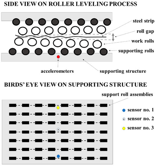
Figure 2.
Drawing of roller leveling process with approximate positions of accelerometers on the supporting structure beneath the lower supporting rolls.
The roller leveling process studied is used for strips of cold steel at the SSAB steel mill in Raahe, Finland. The properties of the 752 steel strips analyzed in this study are diverse, as shown in Table 1. The yield strength, strip thickness, width, and length were 210–1640 MPa, 1.98–15.21 mm, 861–1875 mm, and 68–1161 m, respectively. Sheets are cut from the strip on the production line after the leveler simultaneously with the one-pass leveling process by using a flying shear. The cutting of sheets causes shocks which are conducted to the leveler and emerge as peaks in the monitored acceleration signals. The number of cut sheets in a single strip was 4–465 during the measurement campaign that lasted 37 days.

Table 1.
Information on process parameters, measurements, and computing resources in the study.
2.2. Vibration Measurements
Three accelerometers were stud-mounted on the supporting structure beneath the lower supporting rolls of the leveler. The acceleration was measured horizontally in the cross direction compared with the direction of the roller track. The type of the accelerometers used was SKF CMSS 787A-M8, which has a frequency response from 0.7 Hz to 10 kHz with ±3 dB deviation. The measurement hardware included an NI 9234 data acquisition card and an NI CompactRIO for data acquisition. The sampling rate was 25.6 kHz and the only filter used at the hardware level was the built-in antialiasing filter of the data acquisition card. The measurement system was calibrated using a hand-held calibrator.
2.3. Data Preparation
Vibration was measured continuously during the measurement campaign, and therefore the data included the steel strip leveling periods and other insignificant periods. The leveling events of individual strips were identified from this data manually by combining the time stamps of the measurements with the production data of the factory. The data were also cleaned by removing events that included long periods of inactivity in the leveler and by removing the signal parts distorted by the breaks in the current feed of the measurement system. A more detailed description for the data preparation is provided in [4]. The acceleration signals represented in Figure 1 have undergone the data preparation process.
2.4. Signal Filtering and Feature Generation
The frequency domain filtering of acceleration signals by using various frequency bands is described in Section 2.4.1. The methods for the computation of time domain and frequency domain features are described in Section 2.4.2 and Section 2.4.3, respectively. In this study, the feature values were first computed in short time windows from the duration of the entire leveling event producing a time series for each feature. The time series was then further compressed to statistical values to represent the complete leveling process of each strip. In addition, these statistical values were further processed with different mathematical transformations to identify possible non-linear correlations between the vibration features and the properties of steel strips. The lengths of the time windows in feature calculation and the number of frequency bins in amplitude spectra were selected based on a preliminary correlation analysis, the results of which are not included here. The full set included 144,000 different features extracted from the acceleration signals.
2.4.1. Filtering
The time domain signals of the complete leveling event were multiplied by Tukey window function with 10% taper before filtering the signals in the frequency domain. The Fast Fourier Transform (FFT) was then used to transform the vibration signals into the frequency domain, where the unwanted frequency components were removed by multiplying the corresponding complex numbers by zero. This procedure enables the selection of certain frequency range and the removal of all the frequency components outside the specified range. After this procedure, the signals were transformed back into the time domain by using the inverse FFT. A similar approach was used in [21], for example.
The acceleration signals were filtered using 39 frequency bands, which are shown in Figure 3. The objective was to divide the full applicable frequency range into different-sized bands that each consisted of 5%, 10%, or 20% of the full range. The applicable range (0–10 kHz) was selected based on the frequency response specifications of the accelerometers introduced in Table 1.
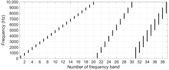
Figure 3.
Illustration of 39 frequency bands used in signal filtering.
To demonstrate the effects of signal filtering, plot A in Figure 4 shows the acceleration signal from sensor no. 1 during a leveling event, where a strip with properties (7.01 mm, 1482 mm, 1038 MPa) was processed. Plots B, C, and D show the corresponding filtered signals using frequency bands 0–0.5, 3–4, and 7–9 kHz, respectively. The signals reveal the peaks and changes in the amplitude differently when different frequency bands are applied. For example, the shocks caused by the flying shear, which are shown by the peaks, are weaker in plot B when compared with plot C. The period with low amplitudes after 1100 s was presumably caused by a short break in the leveling operation.
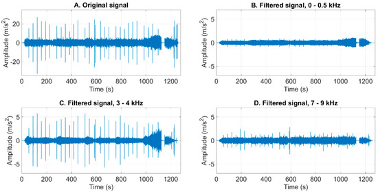
Figure 4.
Original signal and filtered signals using three frequency bands.
2.4.2. Generation of Time Domain Features
The correlations between steel strip properties and signal characteristics in the roller leveling process are largely unclear and not widely studied based on our knowledge, but more limited observations were presented in [4,6]. Therefore, the generation of a relatively large set of candidate features gives a well-founded basis for the solution in this study. Twenty statistical features were computed from three original signals and their 39 frequency-filtered versions. These features are reasonable in practical applications due to their minor requirements for computing capacity. Most of the features are based on the lp norm which is also named as the generalized norm [20]. It is defined by
where the real number α represents the order of derivative, x is the displacement, N is the number of data points in the time window, and the real number p is the order of the norm. In this study, only the acceleration signals (x(2)) were used.
The set of twenty candidate features is presented in Table 2. Several lp norms and ratios of lp norms were computed. Additionally, features which describe the shape of probability distribution, such as the kurtosis (2) and skewness (3) of signal values, and 95th percentile of absolute signal values, were calculated. Kurtosis and skewness are defined by

Table 2.
Definitions for twenty features.
The features were computed in 10-s segments (or time windows). After each segment of the complete leveling event was processed, the median (P50) and upper quartile (P75) of the features were computed to get typical values for the leveling event. The values were min-max scaled to range 0–1 based on all the leveling events in the data set. The P50 and P75 values were then also transformed by using square, cube, square root, and cube root on them. Altogether, 8000 features were therefore computed from each measurement position (or acceleration signal) with this approach.
Figure 5 illustrates the features l0.5, l2, l10, and l10/l2 calculated from the filtered signal using the 3–4 kHz band during the leveling event demonstrated also in the previous section. The plots show that in some cases the median describes the typical operation more appropriately than the upper quartile, and sometimes vice versa. In plot A, it could be interpreted that the upper quartile of l0.5 around the value 0.9 represents the typical values during leveling. Then again, the median of l10 around 0.15 in plot C represents the amplitude level of the typical vibration during roller leveling, whereas the upper quartile around 0.45 is markedly affected by the shocks caused by the operation of flying shear. The tapered beginning and end of signals (see Figure 4) caused by the windowing of the complete signals (see Section 2.4.1.) were removed before the feature computation.
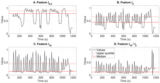
Figure 5.
Features sensitive to different phenomena in signals are shown together with their median and upper quartile values. The presented signal was filtered using the 3–4 kHz frequency band.
2.4.3. Generation of Frequency Domain Features
Amplitude spectra were computed in one-second segments (or time windows). The number of frequency bins in FFT was set NFFT = 2560, which results in 10 Hz frequency resolution with the applied sampling rate given in Table 1. The 1000 bins corresponding to the frequencies 10–10,000 Hz were selected for the analysis based on the accelerometer specifications (see Section 2.2). The length of segments and the number of frequency bins were selected based on experimenting on different settings and analyzing correlations between the features and steel strips. Short windows can be justified based on the dynamic nature of the leveling process.
Eight statistical features including the percentiles (P25, P50, P75, P95), and maximum, mean, kurtosis, and skewness were computed from each frequency bin resulting in 8000 features. Like in the approach in the previous section, the features were first scaled to range 0–1 based on all leveling events and then transformed by using square, cube, square root, and cube root on them as well. Altogether, 40,000 features were thus computed from each measurement position.
Figure 6 demonstrates the amplitude spectra computed in the successive one-second time windows from the same signal as in two previous sections. In this signal, relatively high amplitudes were present at the frequency bins around 1 kHz almost continuously. Some of the shocks inflicted presumably by the flying shear are manifested especially around 4–5 kHz region in this signal.
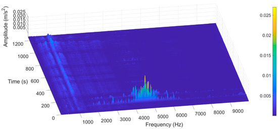
Figure 6.
Amplitudes of frequency components (or bins) computed in one-second time windows during one leveling event.
2.5. Feature Selection Algorithms
Feature selection is one of the most significant parts in the analysis of high-dimensional data. The irrelevant parts of the feature set are removed while the parts with potentially useful information are kept. The methods tested in this study can be categorized as filters and wrappers [47]. Section 2.5.1 describes the information-theoretic criteria (filters) used to pre-select a subset before applying the exhaustive search approach to select the feature combinations for models. Since exhaustive search is not a practical approach for high-dimensional sets, two wrappers were tested as an alternative approach to the feature selection using the entire feature set. Section 2.5.2 describes the sequential forward selection and floating search algorithms. Each algorithm was used to select d = 10 features at most in this study.
2.5.1. Information-Theoretic Filters
Mutual information is a measure of dependence based on information theory and the notion of Shannon’s entropy [48]. The mutual information of two discrete random variables is defined as
where p(·) denotes the probability distribution function of a discrete random variable or pair of variables, and N is the number of data points. Variable xi is the ith candidate variable and y is the target variable. Mutual information measures the quantity of information about the target y that is provided by the variable xi. This method makes no assumptions regarding the structure of the dependence between the variables, such as the linearity. The densities p(·) are unknown and difficult to estimate. The methods used for the estimation include the quantization of variables and the approximation of their densities with a non-parametric method such as Parzen windows [22]. In this study, the variables (or features) were quantized in ten bins.
Various filters using heuristic criteria based on the mutual information have been introduced in the literature [29]. Brown [49] showed that many of them can be expressed by using a common functional form
where β and γ are configurable parameters varying in [0,1] and J is the criterion value. While xi is the ith variable being evaluated, xk represents the already selected variables, and y is the target variable. The first term I(xi,y) ensures the feature relevance (i.e., mutual information). The second term with the parameter β penalizes the high correlations (redundancy) between variable itself and the existing variables. The third term with the parameter γ depends on the class conditional probabilities.
Six criteria were evaluated in this study including the mutual information, Mutual Information based Feature Selection criterion (MIFS) [50] with two parameter settings, Joint Mutual Information (JMI) [51], Conditional Mutual Information Maximization (CMIM) [52], and Maximum-Relevance Minimum-Redundancy (MRMR) [53]. Table 3 shows the parameter values which were used in the tested criteria (5) in this study. CMIM has a slightly different form, which can be written as [29]
where S is the set of currently selected features.

Table 3.
Tested parameter values for β and γ in different criteria.
After the dimension of the original feature set was reduced by using the information-theoretic criteria, all the selected subsets of features (i.e., six sets by six criteria) were tested separately as the explanatory variables in the models by using the exhaustive search. Exhaustive search finds the optimal feature subset but suffers from “the curse of dimensionality” [54]. Therefore, its use is practical on relatively low-dimensional feature sets only. The feature subsets, which optimized the model performance, were selected as the sets of explanatory variables in the models. The criteria for model performance evaluation are described in Section 2.6.3.
2.5.2. Wrapper Applications
Two different alternatives were tested in this study. Sequential forward selection [27] is a widely used suboptimal search procedure for feature selection due to its simplicity and speed. The features are included in progressively larger subsets so that the prediction performance of the model is maximized. The selection terminates when the selected subset has the desired number of features. The method suffers from the “nesting effect,” i.e., the subset of k best features must include also the subset of k − 1 best features, and so forth. The subset of k features that is the best together in truth may differ from the selected subset.
The sequential floating search method was presented in [55]. It overcomes the “nesting effect” of forward selection by dynamically backtracking after each sequential forward step by using the sequential backward selection. When a new feature is added to the current feature set, the algorithm attempts to remove one feature at a time to discover a better subset. If the current feature set evaluated includes more features than wanted (>d), the algorithm stops. Nakariyakul and Casasent [28] further improved the algorithm by including an additional search step (i.e., replacement step) to check whether removing any feature in the currently selected feature subset and adding a new one to the resultant subset at each sequential step can improve the current step. This improved version of the floating search algorithm was used in this study.
2.6. Regression Modeling
The correlations between the statistical features of acceleration signals and steel strip properties can be linear or non-linear, and therefore, both assumptions were considered in model identification. Section 2.6.1 presents MLR, which has the linear structure, and Section 2.6.2 describes GRNN, which is free from the linearity assumption. The performance of the models was assessed based on Root Mean Squared Error of prediction (RMSE), Variance Inflation Factor (VIF), and correlation coefficient (Rxy), which are presented in Section 2.6.3. Finally, Section 2.6.4 introduces the approach to model validation.
2.6.1. Multiple Linear Regression
In multiple linear regression, the response variable of the model is considered as a linear combination of certain explanatory variables. MLR models the relationship between two or more explanatory variables and a response variable by fitting a linear equation to observed data. The MLR model with k variables can be defined by
where j = 1, 2, …N, N is the number of observations, y denotes the value of the response variable, x is the value of an explanatory variable, β0 is the intercept, β1–βk are the regression coefficients to be estimated, and ε is the error term. Least squares fitting is used for model identification.
2.6.2. Generalized Regression Neural Network
The generalized regression neural network is a memory-based network, which includes a one-pass learning algorithm with parallel structure. GRNN approximates any arbitrary function between input and output vectors and draws the function estimate directly from the training data. The network configuration consists of four layers, which include the input layer, pattern layer, summation layer, and output layer [56]. Each input unit in the input layer corresponds to individual observed parameters. The input layer is fully connected to the pattern layer, where each neuron represents a training pattern and its output is a measure of the distance of the input from the stored patterns. The pattern layer is connected to the summation layer, which has two different types of summation including S-summation neuron and D-summation neuron. S-summation neuron determines the sum of the weighted outputs of the pattern layer, whereas the D-summation neuron determines the unweighted outputs of the pattern neurons. The connection weight between the ith neuron in the pattern layer and the S-summation neuron is yi, which is also the target output value corresponding to the ith input pattern. The connection weight for D-summation neuron is unity. The output layer divides the output of each S-summation neuron by that of each D-summation neuron. Therefore, a predicted value ŷ(x) to an unknown input vector x can be expressed as [56]
where N and xi represent the number of training patterns (or observations) and the ith training input pattern stored between the input and pattern layers, respectively. The Gaussian D function is defined as
where p indicates the number of elements of an input vector. The xj and xij represent the jth element of x and xi, respectively. The parameter ζ is referred to as the spread parameter, the appropriate value of which is often heuristically defined. The tested values for ζ included (0.01, 0.05, 0.1, 0.2, 0.5, 0.7, 1, 1.5) and newgrnn function in Matlab® was used for model training in this study.
2.6.3. Model Performance Evaluation
Three criteria were used to evaluate the models in this study. The predictive performance of the models was evaluated by using RMSE, which is defined by
where yj, ŷj, and N are the observed value, the predicted value and the total number of observations, respectively.
Multicollinearity in the models with several explanatory variables can be a serious problem [24]. Therefore, VIF of explanatory variables in the models was assessed by
where Ri2 is the coefficient of determination from a regression of explanatory variable xi onto all the other explanatory variables. If Ri2 is close to one, then collinearity is present and VIF will have a high value. As a rule of thumb, a VIF value that exceeds 5 or 10 indicates a problematic amount of collinearity [24].
Pearson’s correlation coefficient was used to evaluate the linear correlation between model predictions and the observed values in Section 3.2.5. Additionally, the method was used in Section 3.1 to get information on the correlations between the signals and the evaluated steel strip properties. The correlation coefficient for two variables x and y is defined by
2.6.4. Model Validation
The models were validated using the repeated random sub-sampling validation aka Monte Carlo cross-validation [57], where the observations in the data set are split randomly into training and test sets multiple times. The response variables (yield strength, width, and thickness) were min-max scaled to range 0–1 to make the various models comparable. Feature combinations were selected based on the lowest mean of RMSE in cross-validation test sets. Thereafter, the combinations that had VIF above 5 were rejected. Moreover, the models that had larger than 0.02 difference in the mean RMSE between test and training sets were rejected because the models were considered overfitted.
Two approaches to data splitting were tested in the feature selection stage:
- When (a) MLR was applied with the forward selection, and (b) MLR and GRNN were applied with the exhaustive search, the data set was split 50 times into training and test sets, where 80% of the points were used in the training sets and the rest were used in the test sets.
- The data were split 10 times with the same split sizes as in approach 1 when (a) MLR was applied with the floating search, and (b) GRNN was applied with the forward selection.
These different approaches to data splitting were applied due to the major computational burden caused by the high-dimensional feature set. The computational times are demonstrated in Section 3.2.2. After each model had its feature combinations selected, all the models were further compared by using the same 50 random data splits (80%/20%) to have a fair comparison. The results are presented in Section 3.2.1.
The GRNN were tested with all the values of ζ described in Section 2.6.2 and the value of ζ resulting in the lowest RMSE was selected. However, initially during the forward selection, only ζ = 0.05 was used in order to achieve faster computation. Floating search was not used due to its high computational cost.
After the model structure and features were selected based on both the RMSE and VIF criteria (Section 3.2.1) and residual analysis was done (Section 3.2.4), the final models were further validated by selecting 20% of the data to external validation set. This set included temporally successive steel strips. The rest of data points were used in cross-validation, where 50% of the remaining data points were used for training and the rest for test sets. As suggested in [58], the random data split was repeated 3N times, where N is the number of data points (i.e., steel strips).
2.7. Moving Mean and Range Charts
When all the variations in a process arise from random or common causes and none of them are attributable to assignable, non-random or special causes, the process is in statistical control. Various control charts have been introduced to process monitoring and the traditional approach is to use the mean and range charts together [45]. The idea is to monitor the process in samples instead of single observations of the monitored variable. When these samples appear at warning or alarm zones defined by limits, anomalous performance in the process could be detected.
In many industrial processes, the nature of production or analytical methods cause long time intervals between consecutive results. This is valid also in steel strip leveling where the process lasts several minutes for a single steel strip and there may be breaks between successive strips. Therefore, a more practical approach is to use moving mean and range charts in the monitoring [45]. The moving (or sliding) window approach reduces the time to get new monitoring results when compared with an approach where each sample consists of fully independent observations.
Data from the previous operation when the process was in control are used to identify the limits for the charts in the presented approach (see Figure 1). In the moving mean chart, the warning and alarm limits can be defined with various approaches with the assumption that the data follow a normal distribution during the typical operation. In this study, the monitored variables are residuals of regression models and they have relatively large variance due to the model and data quality issues. Therefore, the warning and alarm limits were set to ±2σ and ±3σ (two and three standard deviations) on both sides of the historical mean of the monitored variable. For the monitoring purpose, the sample size (n) is commonly selected in the range n = 4–12 [45]. In this study, n = 5.
The control limits in moving range charts are asymmetrical about the mean range (), which is defined based on the ranges of separate time windows. Based on the selected sample size, the following constants given in [45] (p. 348) were used in the charts in this study: D′0.001 = 2.34, D′0.025 = 1.81; D′0.975 = 0.37; D′0.999 = 0.16. The upper and lower alarm limits are , , and the upper and lower warning limits are , , respectively.
3. Results
Section 3.1. reveals the highest linear correlations between the steel strip properties and features computed based on the signals measured from different positions on the machine structure. The modeling results are presented in Section 3.2. The approach to the monitoring of the roller leveling process is demonstrated in Section 3.3.
3.1. Correlation Analysis
Table 4 shows the maximum linear correlations between the steel strip properties and tested features. The features are grouped into the features calculated from (1) full bandwidth signals, (2) band-pass filtered signals, and (3) frequency components. Table 5 provides the descriptions for the features with the strongest correlations.

Table 4.
Strongest correlations between features and steel strip properties.

Table 5.
Features with strongest correlations to steel strip properties. Pk stands for the kth percentile and Xj stands for the amplitude of frequency j.
The results show that yield strength had the strongest correlations with the features computed from sensor no. 2. The width of steel strip had stronger correlations with the features from the signals on the sides of the roller track (sensors no. 1 and 3). However, the correlations were just mediocre (≤0.58). The location of a sensor did not have such a clear effect on the (absolute) correlations with thickness.
Table 4 and Table 5 reveal that especially the low frequency range (0–500 Hz and 500–1000 Hz) in the signals correlated strongly with the strip thickness. Yield strength had the strongest correlations with the features computed from the frequency components, whereas the thickness had the strongest correlations with the features from band-pass filtered signals. The strip width had almost equal correlations with the features from band-pass filtered signals and the features from frequency components. In general, these results indicate that the band-pass filtered signals and single frequency components correlated with the steel strip properties stronger than the full bandwidth signals. Figure 7 shows the scatter plots for each steel strip property and the feature that had the strongest correlation with it.
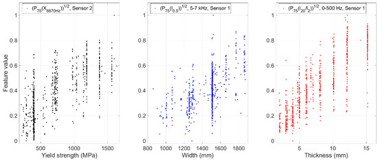
Figure 7.
Scatter plots between the studied steel strip properties and the features with the strongest correlations with them.
3.2. Estimation of Steel Strip Properties
3.2.1. Performance Criteria in Feature Selection
The left side in Figure 8 shows the RMSE of test sets in cross-validation during the selection of 1–10 features with each of the tested methods. The estimation of yield strength based on MLR with floating search was ended on the sixth feature due to the high computation time and the increased VIF values, as shown in Figure 9. The right side of Figure 8 shows the difference in RMSE between the test and training sets. The difference higher than 0.02 was considered as a sign of overfitting. In general, GRNN with forward selection resulted in the lowest RMSE, but as shown on the right, these models had the symptoms of overfitting already with 3–4 features. The same effect was present in GRNN when features were selected based on the information-theoretic filters and exhaustive search. MLR did not suffer from overfitting and the best performing models were obtained by using the floating search or forward selection algorithms.
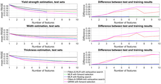
Figure 8.
RMSE of the best performing models in feature selection on the left. The difference between test and training results on the right gives indications about overfitting in model training.
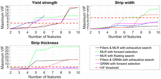
Figure 9.
Maximum variance inflation factor (VIF) in the feature subsets selected by different approaches.
Figure 9 illustrates the maximum VIF in each model with the selected features when it was computed based on the complete set of 752 steel strips. In this approach, VIF < 5 gives an indication of the acceptable amount of collinearity in the explanatory variables of the models. MLR with forward selection reached the VIF threshold already when 5–6 features were selected. In the modeling of yield strength, also the floating search and GRNN with forward selection reached the limit already with four and five features, respectively. In thickness estimation, GRNN with the combination of filters and exhaustive search exceeded the limit on the fifth feature too. In the width and thickness estimation, some of the feature subsets selected by different approaches never reached the threshold with the combinations of 2–10 features. This suggests that even a higher number of features could perhaps be selected without compromising the objective of low multicollinearity in explanatory variables.
3.2.2. Computation Time in Feature Selection
Figure 10 illustrates the computation time spent in the feature selection using the methods described. The results are not exactly commensurate, because the load on the server used for computations was not fixed. The server includes two 2.8 GHz 10-core E5-2680v2 Xeon processors with 512 GB memory. The wrapper methods were applied by using 12 workers for parallel computing to speed-up the cross-validation iterations. The information-theoretic criteria were computed by using a single processor.
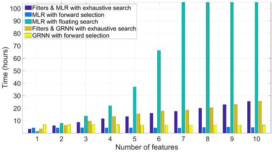
Figure 10.
Computation times in feature selection. Computation times above 105 h are omitted for clarity.
The results indicate that forward selection was generally the fastest method. It was slightly faster with MLR than GRNN although these methods had 50 and 10 cross-validation iterations in the selection stage, respectively. In addition, only one spread parameter (ζ = 0.05) was tested in GRNN in the feature selection stage to reduce the computation time, as explained in Section 2.6.4.
The computation time with the information-theoretic selection and exhaustive search was almost the same using both the MLR and GRNN. This is explained by the relatively small set of candidates (i.e., ten features) in the exhaustive search. The presented computation time is the sum of the computation times spent in the exhaustive search using the feature sets given by each of six criteria separately. If only one information-theoretic criterion had been tested, the computation time would have been markedly lower.
The floating search algorithm was clearly the slowest one. This can be explained by the time-consuming replacement steps. The number of replacement steps also varies based on the studied data set, and therefore, its prediction is difficult. The presented results for floating search describe the average computation times of the feature selection for the strip thickness and width estimation. In the other feature selection approaches, the estimated variable does not influence the computation time. The computation time for the selection of 10 features with floating search took approximately two weeks, which indicates it is the least practical method considering the computational burden.
3.2.3. Selected Features
As shown in Section 3.2.1, the features were selected by minimizing the test RMSE and limiting the difference between test and training RMSE to 0.02 and the VIF to less than five. Therefore, each of the selected models was MLR, the selected features of which are provided in Table 6.

Table 6.
Features used as explanatory variables x1–x10 in MLR models. S1, S2, and S3 stand for the sensors no. 1, 2, and 3, respectively.
The model for yield strength included four features selected based on the forward selection algorithm. The feature selected first was the one with the highest linear correlation with the yield strength (see Table 4 and Table 5). All the selected features were computed from separate frequency components and each of three sensors were included.
The features for strip width and thickness were selected by using the floating search algorithm. Both models included 10 features, but interestingly none of them were the same between the models. The strip width model included mostly features computed from the frequency components, whereas the thickness model included six features from the band-pass filtered signals and four features computed from the frequency components. The selected features in each model were computed from the signals produced by all three sensors. In addition, none of the models included features computed from the full bandwidth signals.
3.2.4. Residual Analysis
Figure 11 shows the RMSE of the selected models fitted on the complete data set of 752 steel strips by using the original dimensions of the strip properties divided into specific intervals shown as bins. The bin sizes are 50 MPa, 50 mm, and 0.5 mm for yield strength, width, and thickness, respectively. The bars show the RMSE in each bin and the crosses show the number of strips belonging to these bins.
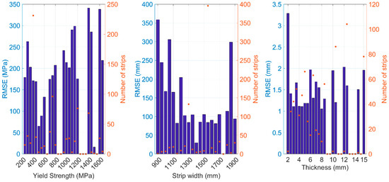
Figure 11.
RMSE of models fitted on the complete data set of 752 steel strips in bins.
The yield strength had relatively high RMSE in general and it was slightly magnified with the higher yield strengths. The strip width had the highest RMSE with the narrow strips and the singular bin with three strips centered at 1850 mm. The strip thickness had high RMSE on the bin corresponding to the lowest thickness (up to 2 mm).
To improve the selected models, the steel strips with 1200 mm width or less and the strips with 2 mm thickness or less were removed from the data set in the next stage. Figure 12 shows the scatter plots between the reference values and estimated values as black triangles based on the models trained by using all 752 strips. The remaining 690 strips after the removal of the strips mentioned are illustrated by the triangles with red dots inside. Figure 13 shows the normal probability plots of the residuals for the models trained based on the remaining 690 strips. The plots show that most of the residuals are relatively close to normal distribution but the points at both ends deviate from the dashed line indicating normal distribution.
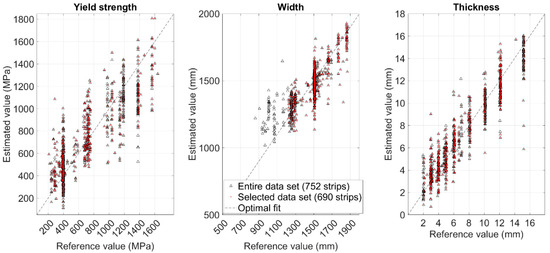
Figure 12.
Scatter plots between the reference values and estimated values using the full set of 752 strips and the strips remaining after the removal of narrow (≤1200 mm) and thin (≤2 mm) strips.
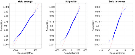
Figure 13.
Normal probability plots of the residuals based on models fitted on the remaining 690 points after the removal of narrow and thin strips.
3.2.5. Validation of Selected Models
The 690 steel strips used in model validation had the yield strength 210–1639 MPa, width 1223–1875 mm, and thickness 2.04–15.21 mm. The strip properties were min-max scaled to range 0–1 in order to get comparable modeling results. Table 7 shows the results of the cross-validation and external validation. The data split was done as explained in Section 2.6.4. The results reveal that the model for thickness estimation had the best performance from the models based on both RMSE and Rxy. The model for yield strength had slightly higher Rxy than the width model, whereas the model for width had slightly lower errors based on RMSE. The performance on the external validation set was slightly better when compared with the cross-validation sets in general.

Table 7.
RMSE and Rxy criteria (µ ± σ) in cross-validation (CV) and external validation sets for each strip property by using multiple linear regression.
Table 8 provides the model coefficients when the complete cross-validation set (552 strips) was used in model training. The 138 strips in the external validation set were not used in model training, because these strips were selected as the independent data set for the demonstration of roller leveler monitoring shown in Section 3.3. The significance test for linear regression [24] indicated that p-values for the regression coefficients were low (p-value << 0.05) apart from the intercept (β0) in the yield strength model (p-value = 0.18). Therefore, the regression coefficients can be considered significant for the models.

Table 8.
Model coefficients (β0–β10) for the estimation of each strip property.
3.3. Statistical Process Control in Roller Leveler Monitoring
3.3.1. Demonstration with Industrial Data
The moving mean and range charts were used to monitor the difference between the estimated and reference values with the goal to detect deviations from the expected operation. The MLR models were trained and the limits for the charts were identified based on the cross-validation set of 552 steel strips presented in the previous section. The alarm and warning limits for each model are illustrated in Figure 14 using thick and thin dash lines, respectively.
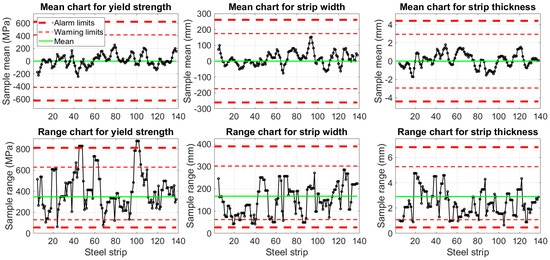
Figure 14.
Roller leveler monitoring based on moving mean and range charts using the external validation points.
Figure 14 demonstrates the monitoring based on the 138 steel strips in the external validation set using the original values of the steel strip properties. Based on the mean charts, the operation remained inside the warning limits and was therefore in control. In the range chart of yield strength, the upper alarm limit was crossed around strips number 45 and 100, which indicates that the process was not in control. In the range charts of strip width and thickness, only the lower warning limit was exceeded by a few samples. However, it is questionable if the lower limits for range are useful in practice because the monitored variable is a sample of residuals: The low range in a sample due to low residual values indicates that the model has a good predictive performance. Furthermore, some crossings of limits can be expected as the data were not exactly normally distributed, as shown in Figure 13.
3.3.2. Simulation of Anomalies with the Thickness Model
Two types of anomalies in the signals, including drifts and temporary anomalies, were simulated with the thickness model to demonstrate the monitoring performance in case the signals give signs of deviating operation. The positive drift was simulated by multiplying the actual value of variable x1 by a constantly increasing value starting from the 6th point and ending at the last point of the period (138th point). The applied coefficient increased from 1.01 to 2.33 with the step size 0.01. The negative drift in x1 was simulated similarly by using a decreasing coefficient from 0.99 to −0.33 with step size 0.01. Moreover, the simultaneous positive drifts in all explanatory variables were simulated by multiplying all the variables with the increasing coefficients. The positive and negative drifts in variable x1 are illustrated in Figure 15.
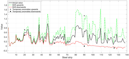
Figure 15.
Different anomalies in the explanatory variable x1 of thickness model.
In addition, temporary anomalies were simulated with three approaches. In this case, the values of variable x1 for the strips number 20, 55, 90, and 135 were multiplied by 1.2, 1.5, 2, and 2.5 to produce anomalies upwards, and the values were multiplied by 0.8, 0.5, 0, and −0.5 to produce anomalies downwards, respectively. In the third case, the values of all ten explanatory variables for the same strips were multiplied by 1.2, 1.5, 2, and 2.5, respectively. The temporary anomalies in variable x1 are illustrated in Figure 15.
The effects of the drifts are demonstrated in Figure 16. Based on the charts, the process got out of statistical control in each simulation. The warning limits were exceeded in the moving mean charts earlier during the drifts upwards in comparison to the drift downwards. The drifts in all explanatory variables resulted in the clearest deviation outside the chart limits. In the range charts, the drifts on all explanatory variables caused several events where the upper alarm limit was exceeded. The drifts on x1 alone caused several crossings of the upper warning limit and one period of samples above the upper alarm limit around the 110th strip in the case of drift downwards.
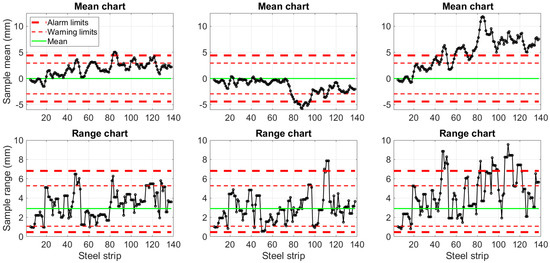
Figure 16.
Control charts for the strip thickness in cases with drift upwards in the first explanatory variable (left), drift downwards in the first explanatory variable (middle), and drift upwards in all ten explanatory variables (right).
Figure 17 shows the effects of the temporary anomalies on the monitored sample means and ranges on the charts for the thickness model. This type of anomaly was not indicated as clearly as the drifts in Figure 16. However, out-of-control events emerged in the range chart around the strip number 90 in the case of the anomaly upwards. The samples in the mean charts remained between the warning limits. These results confirm that the moving mean is not sensitive to the relatively small momentary changes. Instead, this suggests that the approach is more suitable for the monitoring of long-term changes such as the drifts.

Figure 17.
Control charts for the strip thickness in cases with temporary anomalies upwards in the first explanatory variable (left), temporary anomalies downwards in the first explanatory variable (middle), and temporary anomalies upwards in all ten explanatory variables (right).
4. Discussion
4.1. Significance of Selected Features
The features were selected computationally without previous knowledge on their exact relation to the monitored steel strip properties. However, the results suggest that the steel strip properties and the characteristics of the vibration signals had strong correlation with each other. The clearest indication was given by the correlations of individual features especially with strip thickness in Table 4 (Section 3.1). The strip width generally had the lowest correlations with individual features, but the signals from the sides of the track had slightly stronger correlations than the one in the middle. This indicates that the sensor location is important for the width estimation. On the contrary, the signal from the sensor in the middle had stronger correlations with yield strength compared with the signals from the other two sensors. These correlations are perhaps affected more by the measurement procedure than by the physical properties of the steel strips. When the features were combined from all signals by using MLR, the correlations were improved as shown by the results in Table 7. This indicates that the features were relevant for the statistical modeling purpose, but more research is required on their practical application.
The tested feature selection approaches were suboptimal, which has a great influence on the selected combinations in high-dimensional data sets. The size of partitions in cross-validation and the selected performance criteria have some influence on the features selected based on the wrapper methods. The selected feature combinations are therefore case-specific to the approach used.
The results reveal that the approach benefitted from the frequency filtering and from the use of frequency bins before calculating the statistical features. The explanatory variables for strip thickness included many features sensitive to shocks, such as l10/l2, l∞, and l10, which also indicates that the shocks caused by the flying shear influenced the trained models. The shocks caused by cutting presumably improved the model accuracy, because the effects of shocks in the signals correlate strongly with strip thickness; see also [6].
4.2. Practical Challenges
In the presented approach, complete leveling events were analyzed without information on the momentary parameters of the machine. The leveling process is not stationary, and it has different stages, as shown by the signal in Figure 4. The computed feature values, which describe the whole event in its entirety, thus have a relatively high variance. This was shown by the model performance and especially the overfitting of GRNN (see Section 3.2.1) can be partially explained by such variation.
The duration of the whole leveling event can be relatively long, which is shown in Figure 4. This causes computational burden to signal filtering and feature extraction. Therefore, the practical monitoring should be done based on short segments, in the order of a few seconds. To identify the appropriate segments reliably, additional variables of the machine operation would be needed. Moreover, signal downsampling techniques [59] or efficient algorithms for data stream processing [60] could provide alternative solutions if the loss of essential information carried by the signals can be avoided.
Moreover, the regression coefficients in MLR with opposite signs (see Table 8) may cancel the detection of deviating operation manifested by many features simultaneously. However, this is not necessarily a major disadvantage, as shown in Section 3.3.2 where the values of multiple features increased in the drift simulation and the deviation was nonetheless detected. It is also possible to define the typical operational ranges for the explanatory variables based on the steel strip properties and other machine parameters which might help in such contradictory situations.
4.3. Suggestions and Future Considerations
The approach could be complemented by acquiring additional information about the operation, such as motor power, rotational speed, or torque signals, which are synchronized with vibration signals. The variance in the features used as explanatory variables in the models (see Figure 7) could be reduced as a result of the more precise identification of the different operational states of the machine. It could be advantageous to identify different models for the start, middle part, and the end of the leveling process. The use of models specific to different rotational speeds or ranges of the strip properties could further improve the modeling accuracy, and tighter control limits could then be defined on the SPC charts. However, the improvement in the accuracy could lead into an increased need for the model updating due to the changes in the machine operation or processed materials. Therefore, the techniques for the model adaptation to different local operating regimes [61], concept drift adaptation [62], and soft sensor adaptation [63] could be useful for the practical application.
The measurements were done only in the horizontal direction. The measurement of vertical acceleration could improve the accuracy of the method, because the forces in that direction are highly dependent on the processed material. Moreover, the correlations in Table 4 showed that the sensors on the side of the track had stronger correlations with strip width than the one in the middle. Additional sensors positioned crosswise across the roller track could improve the width estimation.
The principal target of application for this kind of monitoring would be in the condition monitoring of the machine supporting the CBM approach. If the operation deviated from the expected, a more detailed diagnosis could be initiated. Moreover, the method could be supplemented by the typical operational ranges of the explanatory variables at specific strip width, yield strength, and thickness areas. This would reveal the characteristics of vibration which are deviating from the expected. Increased values on features sensitive to shocks could be the result of local defects in rotating components, for example. An additional target could be the detection of an incorrect steel strip or strip property if the variation in the data was reduced and model accuracy further improved.
5. Conclusions
An approach to the monitoring of industrial roller levelers based on regression models was proposed. The models were used to estimate steel strip properties based on statistical features computed from acceleration signals. The residuals of the models were monitored using moving mean and range charts, the limits of which were identified based on the previous operation of the machine. The results indicate that the approach benefitted from frequency filtering the acceleration signals—either using specific bands or singular frequency bins—before feature calculation. The mathematical transformations of these features further improved their correlation with the steel strip properties, including the yield strength, width, and thickness of the strips. The best feature combinations were identified with wrapper algorithms, but especially the floating search algorithm required a long computation time, which limits its applicability on high-dimensional data sets, such as the used one with 144,000 separate features. The generalized regression neural network suffered from overfitting presumably due to the noisy input data, i.e., the unexplainable variation in the features, whereas multiple linear regression performed well in this respect. The approach to roller leveler monitoring could be further improved with additional information on the momentary operation of the machine, such as motor power or rotational speed. The tested approach could be applicable also on other types of machines, which process materials or have operational parameters that correlate strongly with the measured vibration.
Author Contributions
Conceptualization, R.-P.N.; methodology, R.-P.N.; software, R.-P.N.; validation, R.-P.N.; formal analysis, R.-P.N.; investigation, R.-P.N.; data curation, R.-P.N.; writing—original draft preparation, R.-P.N.; writing—review and editing, R.-P.N. and K.L.; visualization, R.-P.N.; All authors have read and agreed to the published version of the manuscript.
Funding
This research received no external funding.
Acknowledgments
The authors would like to thank the personnel of SSAB Europe in Raahe (Finland) for their collaboration, enabling the measurement campaign and providing the production data for the research during the DIMECC SIMP program (2014–2017).
Conflicts of Interest
The authors declare no conflict of interest.
References
- Sahal, R.; Breslin, J.G.; Ali, M.I. Big data and stream processing platforms for Industry 4.0 requirements mapping for a predictive maintenance use case. J. Manuf. Syst. 2020, 54, 138–151. [Google Scholar] [CrossRef]
- Shin, J.-H.; Jun, H.-B. On condition based maintenance policy. J. Comput. Des. Eng. 2015, 2, 119–127. [Google Scholar] [CrossRef]
- Dunson, D.B. Statistics in the big data era: Failures of the machine. Stat. Probab. Lett. 2018, 136, 4–9. [Google Scholar] [CrossRef]
- Nikula, R.-P.; Karioja, K.; Leiviskä, K.; Juuso, E. Prediction of mechanical stress in roller leveler based on vibration measurements and steel strip properties. J. Intell. Manuf. 2019, 30, 1563–1579. [Google Scholar] [CrossRef]
- Silvestre, E.; Mendiguren, J.; Galdos, L.; Sáenz de Argandona, E. Comparison of the hardening behaviour of different steel families: From mild and stainless to advanced high strength steels. Int. J. Mech. Sci. 2015, 101–102, 10–20. [Google Scholar] [CrossRef]
- Nikula, R.-P.; Karioja, K. The Effect of Steel Leveler Parameters on Vibration Features. In Linköping Electronic Conference Proceedings, Proceedings of the 9th EUROSIM & the 57th SIMS, Oulu, Finland, 12–16 September 2016; Linköping University Electronic Press: Linköping, Sweden, 2018; Volume 142, pp. 433–438. [Google Scholar] [CrossRef]
- Yi, G.; Wang, Z.; Hu, Z. A novel modeling method in metal strip leveling based on a roll-strip unit. Math. Probl. Eng. 2020, 2020, 1–16. [Google Scholar] [CrossRef]
- Galdos, L.; Mendiguren, J.; de Argandona, E.S.; Otegi, N.; Silvestre, E. Influence of Roll Levelling on Material Properties and Postforming Springback. In AIP Conference Proceedings, Proceedings of the 21st International ESAFORM Conference on Material Forming, Palermo, Italy, 23–25 April 2018; AIP Publishing: Melville, NY, USA, 2018; Volume 1960. [Google Scholar] [CrossRef]
- Lahdelma, S.; Juuso, E.K. Signal processing and feature extraction by using real order derivatives and generalised norms. Part 2: Applications. Int. J. Cond. Monit. 2011, 1, 54–66. [Google Scholar] [CrossRef]
- Rai, A.; Upadhyay, S.H. A review on signal processing techniques utilized in the fault diagnosis of rolling element bearings. Tribol. Int. 2016, 96, 289–306. [Google Scholar] [CrossRef]
- Lan, H.; Yan, L.; Xiao, D.; Jiao, Z.; Chen, I.-M. Surface-to-surface calibration of acoustic emission sensors. Sens. Actuat. A-Phys. 2012, 174, 16–23. [Google Scholar] [CrossRef]
- Sikorska, J.Z.; Mba, D. Challenges and obstacles in the application of acoustic emission to process machinery. Proc. Inst. Mech. Eng. E J. Process. Mech. Eng. 2008, 222, 1–19. [Google Scholar] [CrossRef]
- Widodo, A.; Kim, E.Y.; Son, J.-D.; Yang, B.-S.; Tan, A.C.C.; Gu, D.-S.; Choi, B.-K.; Mathew, J. Fault diagnosis of low speed bearing based on relevance vector machine and support vector machine. Expert Syst. Appl. 2009, 36, 7252–7261. [Google Scholar] [CrossRef]
- Laurila, J.; Lahdelma, S. Condition Monitoring by Means of Vibration and Sound Measurements. In Proceedings of the Tenth International Conference on Condition Monitoring and Machinery Failure Prevention Technologies, Krakow, Poland, 18–20 June 2013; pp. 227–245. [Google Scholar]
- Lahdelma, S.; Karioja, K.; Laurila, J.; Ahola, J. Distortion in Acoustic Emission and Acceleration Signals Caused by Frequency Converters. In Proceedings of the Ninth International Conference on Condition Monitoring and Machinery Failure Prevention Technologies, London, UK, 12–14 June 2012; pp. 905–925. [Google Scholar]
- Janssens, O.; Slavkovikj, V.; Vervisch, B.; Stockman, K.; Loccufier, M.; Verstockt, S.; Van de Walle, R.; Van Hoecke, S. Convolutional neural network based fault detection for rotating machinery. J. Sound Vib. 2016, 377, 331–345. [Google Scholar] [CrossRef]
- Lei, Y.; Li, N.; Guo, L.; Li, N.; Yan, T.; Lin, J. Machinery health prognostics: A systematic review from data acquisition to RUL prediction. Mech. Syst. Signal Process. 2018, 104, 799–834. [Google Scholar] [CrossRef]
- Fugate, M.L.; Sohn, H.; Farrar, C.R. Vibration-based damage detection using statistical process control. Mech. Syst. Signal Process. 2001, 15, 707–721. [Google Scholar] [CrossRef]
- Zhang, S.; Zhang, S.; Wang, B.; Habetler, T.G. Deep learning algorithms for bearing fault diagnostics—A comprehensive review. IEEE Access 2020, 8, 29857–29881. [Google Scholar] [CrossRef]
- Lahdelma, S.; Juuso, E.K. Signal Processing in Vibration Analysis. In Proceedings of the Fifth International Conference on Condition Monitoring and Machine Failure Prevention Technologies, Edinburgh, UK, 15–18 July 2008; pp. 867–878. [Google Scholar]
- Nikula, R.-P.; Karioja, K.; Pylvänäinen, M.; Leiviskä, K. Automation of low-speed bearing fault diagnosis based on autocorrelation of time domain features. Mech. Syst. Signal Process. 2020, 138, 106572. [Google Scholar] [CrossRef]
- Guyon, I.; Elisseeff, A. An introduction to variable and feature selection. J. Mach. Learn. Res. 2003, 3, 1157–1182. [Google Scholar]
- Liu, H.; Dougherty, E.R.; Dy, J.G.; Torkkola, K.; Tuv, E.; Peng, H.; Ding, C.; Long, F.; Berens, M.; Parsons, L.; et al. Evolving feature selection. IEEE Intell. Syst. 2005, 20, 64–76. [Google Scholar] [CrossRef]
- James, G.; Witten, D.; Hastie, T.; Tibshirani, R. An Introduction to Statistical Learning with Applications in R; Springer: New York, NY, USA, 2013. [Google Scholar]
- Andersen, C.M.; Bro, R. Variable selection in regression—A tutorial. J. Chemom. 2010, 24, 728–737. [Google Scholar] [CrossRef]
- Al-Ani, A.; Alsukker, A.; Khushaba, R.N. Feature subset selection using differential evolution and a wheel based search strategy. Swarm Evol. Comput. 2013, 9, 15–26. [Google Scholar] [CrossRef]
- Whitney, A.W. A direct method of nonparametric measurement selection. IEEE Trans. Comput. 1971, 100, 1100–1103. [Google Scholar] [CrossRef]
- Nakariyakul, S.; Casasent, D.P. An improvement on floating search algorithms for feature subset selection. Pattern Recognit. 2009, 42, 1932–1940. [Google Scholar] [CrossRef]
- Brown, G.; Pocock, A.; Zhao, M.-J.; Luján, M. Conditional likelihood maximization: A unifying framework for information theoretic feature selection. J. Mach. Learn. Res. 2012, 13, 27–66. [Google Scholar]
- Jardine, A.K.S.; Lin, D.; Banjevic, D. A review on machinery diagnostics and prognostics implementing condition-based maintenance. Mech. Syst. Signal Process. 2006, 20, 1483–1510. [Google Scholar] [CrossRef]
- Sobie, C.; Freitas, C.; Nicolai, M. Simulation-driven machine learning: Bearing fault classification. Mech. Syst. Signal Process. 2018, 99, 403–419. [Google Scholar] [CrossRef]
- Lee, J.; Wu, F.; Zhao, W.; Ghaffari, M.; Liao, L.; Siegel, D. Prognostics and health management design for rotary machinery systems—Reviews, methodology and applications. Mech. Syst. Signal Process. 2014, 42, 314–334. [Google Scholar] [CrossRef]
- Wang, T.; Yu, J.; Siegel, D.; Lee, J. A Similarity-Based Prognostics Approach for Remaining Useful Life Estimation of Engineered Systems. In Proceedings of the International Conference on Prognostics and Health Management, Denver, CO, USA, 6–9 October 2008. [Google Scholar] [CrossRef]
- Kundu, P.; Darpe, A.K.; Kulkarni, M.S. Weibull accelerated failure time regression model for remaining useful life prediction of bearing working under multiple operating conditions. Mech. Syst. Signal Process. 2019, 134, 106302. [Google Scholar] [CrossRef]
- Singh, S.B.; Bhadeshia, H.K.D.H.; Mackay, D.J.C.; Carey, H.; Martin, I. Neural network analysis of steel plate processing. Ironmak. Steelmak. 1998, 25, 355–365. [Google Scholar]
- Das, P.; Datta, S. Exploring the non-linearity in empirical modelling of a steel system using statistical and neural network models. Int. J. Prod. Res. 2007, 45, 699–717. [Google Scholar] [CrossRef]
- Faris, H.; Sheta, A.; Öznergiz, E. Modelling hot rolling manufacturing process using soft computing techniques. Int. J. Comput. Integr. Manuf. 2013, 26, 762–771. [Google Scholar] [CrossRef]
- Dratz, B.; Nalewajk, V.; Bikard, J.; Chastel, Y. Testing and modelling the behaviour of steel sheets for roll levelling applications. Int. J. Mater. Form. 2009, 2, 519–522. [Google Scholar] [CrossRef]
- Liu, Z.; Wang, Y.; Yan, X. A new model for the plate leveling process based on curvature integration method. Int. J. Mech. Sci. 2012, 54, 213–224. [Google Scholar] [CrossRef]
- Yu, G.; Zhai, R.; Zhao, J.; Ma, R. Theoretical analysis and numerical simulation on the process mechanism of two-roller straightening. Int. J. Adv. Manuf. Tech. 2018, 94, 4011–4021. [Google Scholar] [CrossRef]
- Grüber, M.; Kümmel, L.; Hirt, G. Control of residual stresses by roller leveling with regard to process stability and one-sided surface removal. J. Mater. Process Technol. 2020, 280, 116600. [Google Scholar] [CrossRef]
- Sueoka, A.; Matsuzaki, K.; Ryu, T. Polygonal wear of work rolls in a hot leveler of steel making machine. JSME Int. J. Ser. C Mech. Syst. 2002, 45, 673–681. [Google Scholar] [CrossRef]
- Matsuzaki, K.; Sueoka, A.; Ryu, T.; Morita, H. Generation mechanism of polygonal wear of work rolls in a hot leveler and a countermeasure by dynamic absorbers. Int. J. Mach. Tools Manuf. 2008, 48, 983–993. [Google Scholar] [CrossRef]
- Specht, D.F. A General regression neural network. IEEE Trans. Neural Netw. 1991, 2, 568–576. [Google Scholar] [CrossRef]
- Oakland, J.S.; Followell, R.F. Statistical Process Control, a Practical Guide, 2nd ed.; Heinemann Newnes: Oxford, UK, 1990. [Google Scholar]
- Smith, R.P., Jr. Flatness control in coiled plates: Lukens’ wide, cut to length line. Iron Steel Eng. 1997, 75, 29–34. [Google Scholar]
- Kohavi, R.; John, G.H. Wrappers for feature subset selection. Artif. Intell. 1997, 97, 273–324. [Google Scholar] [CrossRef]
- Shannon, C.E. A mathematical theory of communication. Bell Syst. Tech. J. 1948, 27, 379–423. [Google Scholar] [CrossRef]
- Brown, G. A New Perspective for Information Theoretic Feature Selection. In Proceedings of the Twelfth International Conference on Artificial Intelligence and Statistics, Clearwater Beach, FL, USA, 16–18 April 2009; Volume 5, pp. 49–56. [Google Scholar]
- Battiti, R. Using mutual information for selecting features in supervised neural net learning. IEEE Trans. Neural Netw. 1994, 5, 537–550. [Google Scholar] [CrossRef] [PubMed]
- Yang, H.H.; Moody, J.E. Data Visualization and Feature Selection: New Algorithms for Nongaussian Data. In Advances in Neural Information Processing Systems (NIPS); MIT Press: Boston, MA, USA, 1999; Volume 99, pp. 687–693. [Google Scholar]
- Fleuret, F. Fast binary feature selection with conditional mutual information. J. Mach. Learn. Res. 2004, 5, 1531–1555. [Google Scholar]
- Peng, H.; Long, F.; Ding, C. Feature selection based on mutual information: Criteria of max-dependency, max-relevance, and min-redundancy. IEEE Trans. Pattern Anal. Mach. Intell. 2005, 27, 1226–1238. [Google Scholar] [CrossRef] [PubMed]
- Bellman, R. Adaptive Control Processes: A Guided Tour; Princeton University Press: Princeton, NJ, USA, 1961. [Google Scholar]
- Pudil, P.; Novovicova, J.; Kittler, J. Floating search methods in feature selection. Pattern Recognit. Lett. 1994, 15, 1119–1125. [Google Scholar] [CrossRef]
- Kim, B.; Kwon, S.; Kim, D.H. Optimization of optical lens-controlled scanning electron microscopic resolution using generalized regression neural network and genetic algorithm. Expert Syst. Appl. 2010, 37, 182–186. [Google Scholar] [CrossRef]
- Shao, J. Linear model selection by cross-validation. J. Am. Stat. Assoc. 1993, 88, 486–494. [Google Scholar] [CrossRef]
- Baumann, K. Cross-validation as the objective function for variable-selection techniques. TrAC Trends Anal. Chem. 2003, 22, 395–406. [Google Scholar] [CrossRef]
- Proakis, J.G.; Manolakis, D.G. Introduction to Digital Signal Processing; Macmillan Cop: New York, NY, USA, 1988. [Google Scholar]
- Paavola, M. An Efficient Entropy Estimation Approach. Ph.D. Thesis, Acta Univ Oulu C, Oulu, Finland, 2011. [Google Scholar]
- Ruusunen, M.; Leiviskä, K. Fuzzy modelling of carbon dioxide in a burning process. Control Eng. Pract. 2004, 12, 607–614. [Google Scholar] [CrossRef]
- Gama, J.; Žliobaite, I.; Bifet, A.; Pechenizkiy, M.; Bouchachia, A. A survey on concept drift adaptation. ACM Comput. Surv. 2014, 46, 1–37. [Google Scholar] [CrossRef]
- Kadlec, P.; Grbic, R.; Gabrys, B. Review of adaptation mechanisms for data-driven soft sensors. Comput. Chem. Eng. 2011, 35, 1–24. [Google Scholar] [CrossRef]
© 2020 by the authors. Licensee MDPI, Basel, Switzerland. This article is an open access article distributed under the terms and conditions of the Creative Commons Attribution (CC BY) license (http://creativecommons.org/licenses/by/4.0/).