A Boundary Virtual Load Method for Prestress-Field Prediction in Corner-Tensioned Membranes

Abstract

Flexible membrane structures, such as solar sails and membrane reflectors, rely on accurate characterization of in-plane prestress for structural reliability and functional performance. This study proposes a Boundary Virtual Load Method (BVLM) for the semi-analytical prediction of prestress fields in corner-tensioned rectangular membranes. An initial corner-dominated radial stress field is constructed by superposing the stress solutions generated by four corner loads. Residual normal stresses along the nominally free edges are then evaluated, and boundary virtual loads of equal magnitude and opposite direction are introduced to approximate the zero-normal-traction condition. Polynomial representations of these virtual-load distributions are incorporated into the Airy stress-function framework, yielding a boundary-corrected closed-form prestress solution. Comparisons with finite element results for three membrane configurations show that BVLM accurately captures the principal spatial characteristics and aspect-ratio-dependent evolution of the prestress field while requiring substantially lower computational cost for the cases examined. The predicted prestress fields are further incorporated into a free-vibration model that accounts for the added mass of the surrounding air. The resulting natural frequencies generally reproduce the experimentally measured modal-frequency trends, although mode-dependent discrepancies are observed for several modes. The 12 frequency comparisons yield a mean absolute relative error of $8.46\%$, indicating reasonable overall agreement for the approximate analytical formulation. These comparisons provide an indirect dynamic consistency assessment rather than a direct validation of the spatial prestress field. BVLM therefore offers an efficient framework for prestress analysis, preliminary vibration prediction, and parametric design of corner-tensioned membranes.

1. Introduction

Large deployable membrane structures, such as solar sails and membrane reflectors [1], derive their shape stability primarily from an in-plane prestress field rather than from rigid supporting members [2]. Spatial nonuniformity in this prestress field can induce out-of-plane shape deviations and compromise the functional accuracy of the deployed surface. Local prestress deficits may trigger wrinkling [3] and slack regions [4], whereas excessive tension increases the risk of material overload [5]. Such deviations can degrade surface accuracy [6], load-carrying capacity [7], and long-term reliability [8]. Accurate prediction of the prestress field is therefore a primary design requirement rather than merely a post-deployment diagnostic concern. Resolving the in-plane prestress distribution in rectangular membranes with sufficient accuracy is thus essential for structural design and performance control.

The in-plane stress field of a tensile membrane is governed by equilibrium [9,10], whereas its physical response is highly sensitive to compressive stress states. The negligible bending stiffness of thin membranes allows such states to be released through wrinkling or slackening, motivating tension-field and relaxation-based descriptions of the resulting response [11,12]. Within a nonlinear-elasticity framework, Nayyar and co-workers established stress-controlled conditions that distinguish tensile, yielded, and relaxed regions, thereby providing a mechanistic basis for characterizing admissible membrane stress states [13]. Generalized shell formulations developed by Libai [14] further demonstrate the coupled effects of geometric nonlinearity and boundary loading on membrane shape and in-plane stress transfer, highlighting the importance of boundary representation in stress prediction. More recent studies have extended these developments through variational and regularized stress-field constructions. Variational energy regularization has been applied to trace stress evolution in slender membranes under tension [15]; boundary geometry, including edge curvature, has been shown to remotely regulate the direction and distribution of principal stresses [16]; and stress-spectrum-based variational models have been introduced to infer tension-field distributions from principal-strain characteristics while suppressing the numerical oscillations associated with projection-based approaches [17]. Collectively, these studies have advanced tensile-membrane mechanics from idealized analytical descriptions toward more general nonlinear and variational formulations. These formulations primarily address the physical redistribution of membrane stresses when wrinkling, slackening, or other nonlinear responses become relevant.

A gap nevertheless remains between these theoretical developments and the stress-transfer characteristics encountered in corner-tensioned membrane structures. Existing stress-field studies predominantly address uniaxial [9,12,13] and biaxial [14,18] tension states, where the boundary tractions are spatially continuous and comparatively straightforward to prescribe, analyze, and validate. In aerospace applications, prestress is often introduced through concentrated corner loads [19]. Such loading establishes the membrane-wide stress field through highly nonuniform stress transfer [20] and produces effectively discontinuous boundary conditions [21]. The resulting mechanical response is particularly challenging to model: stress concentrations develop near the corners [22,23], while substantial spatial variations arise across the membrane domain. Simplified boundary-loading assumptions may therefore fail to reproduce the actual prestress state with sufficient fidelity [24].

Existing analytical and semi-analytical approaches have made important progress in this area. Representative methods include Airy stress-function superposition and load-ratio-based formulations for concentrated corner loads [25,26], energy-minimization criteria for selecting admissible nonuniform stress paths [27], undetermined-coefficient extensions for membranes with curved or arced boundaries [28], Eshelby-inclusion models for quantifying rigid-insert-induced stress perturbations and wrinkling [29], and segmented polar-field constructions with boundary truncation for improving near-corner accuracy [30]. However, many of these approaches retain idealized descriptions of corner stress transmission and do not explicitly correct the residual boundary effects generated by the initial analytical stress field. Consequently, their predictive accuracy may be limited to local regions or restricted geometric configurations. A unified, design-oriented stress-field model is still needed to simultaneously represent the discontinuous loading characteristics of corner tensioning, maintain mechanical consistency throughout the rectangular domain, and accurately resolve the spatial variation of the Cartesian prestress components required for subsequent structural assessment.

This study develops a Boundary Virtual Load Method (BVLM) for the semi-analytical prediction of the prestress field in corner-tensioned rectangular membranes. The present formulation focuses on predicting the Cartesian prestress components in the taut membrane state within a linear elastic plane-stress framework, rather than modeling stress relaxation or post-wrinkling redistribution. The method is formulated within the Airy stress-function framework. An initial corner-dominated radial stress field is constructed through the superposition of the stress solutions associated with the four corner loads, and the residual normal stresses along the nominally free boundaries are explicitly identified. Boundary virtual loads with equal magnitudes and opposite directions are then introduced to compensate for these residual stresses and approximate the zero-normal-traction condition along the membrane edges. The virtual-load distributions are represented by polynomial functions, from which the associated Airy stress functions are derived to obtain a boundary-corrected closed-form representation of the Cartesian stress components, $({\sigma }_x, {\sigma }_y, {\tau }_{xy})$. The resulting formulation captures the stress-transfer characteristics and boundary effects induced by corner loading while providing a computationally efficient semi-analytical tool for prestress evaluation and structural assessment.

The remainder of this paper is organized as follows. Section 2 presents the BVLM-based prestress-field formulation, including the construction of the initial radial stress field, identification of the boundary-normal stress residuals, and their correction through boundary virtual loads. Section 3 analyzes the resulting stress characteristics and validates the BVLM predictions against FEM results. Section 4 develops the BVLM-based free-vibration formulation and evaluates its predictions using three experimental membrane specimens. Section 5 summarizes the principal findings and engineering implications.

2. Boundary Virtual Load Method for Corner-Tensioned Membranes

2.1. Modeling Assumptions and Corner-Induced Initial Prestress Field

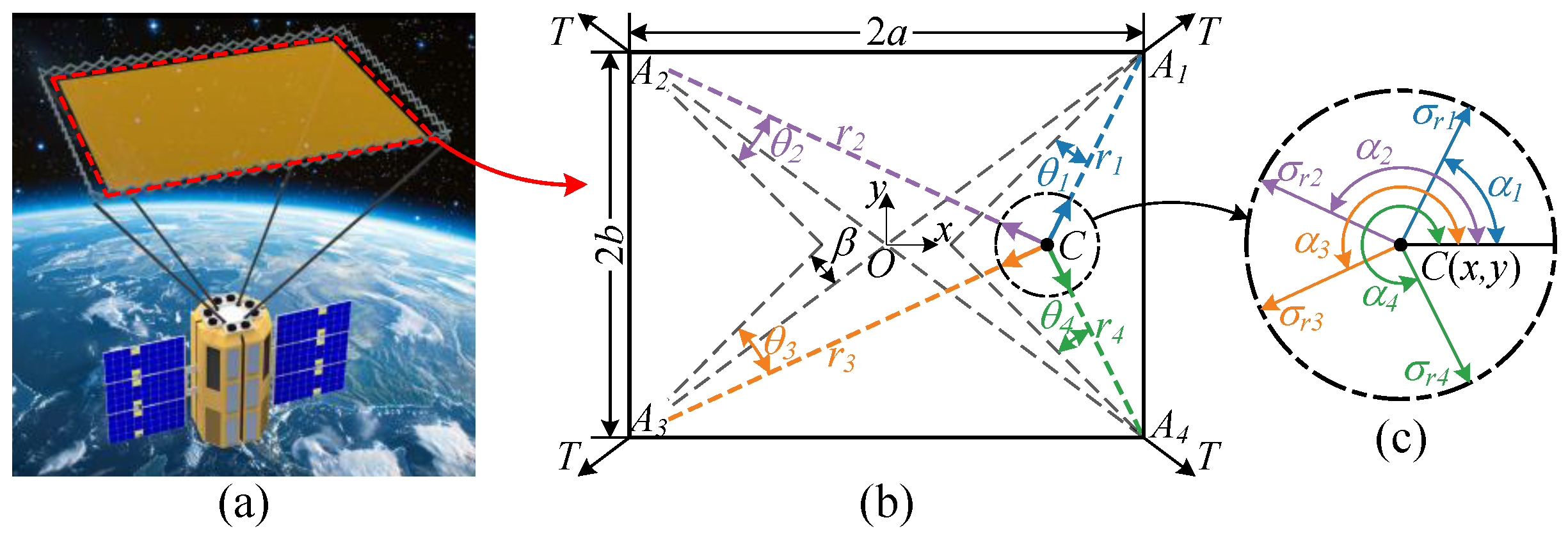
Corner-tensioned large-aperture membrane structures, as shown in Figure 1a, maintain their deployed configurations primarily through in-plane tensile stresses. Their mechanical performance is therefore governed by the prestress field established by corner-applied boundary forces and by the intrinsic material properties of the membrane. The membrane is idealized as a homogeneous sheet without attached substructures, so that the stress-transfer mechanism induced by corner tension can be isolated from local structural perturbations.

The analysis is restricted to the taut prestressed configuration generated by corner tensioning. In this configuration, the membrane boundary follows the prescribed design geometry, while the prestress field represents the corresponding in-plane prestress redistribution within this fixed geometry. Geometrically nonlinear deformation, wrinkling, and slackening are not explicitly resolved, as they are beyond the scope of the present prestress-field construction. This formulation is intended for operating conditions in which the membrane remains globally tensioned; its primary objective is to characterize the spatial distribution of in-plane prestress rather than the post-buckling deformation response.

The corresponding geometric and loading description is defined as follows. As shown in Figure 1b, a rectangular membrane with dimensions $2a\times 2b$ is considered to examine the relationship between the corner-applied tensile forces and the resulting in-plane prestress distribution. A Cartesian coordinate system is defined with its origin at the membrane center, where the x-axis is aligned with the longer edge and the y-axis is aligned with the shorter edge. The four corner points $A_i$ $(i=1, 2, 3, 4)$ are located at $(\pm a,\pm b)$, and identical tensile forces T are applied to these corners along the diagonal directions.

Within the geometric and loading configuration defined above, the initial in-plane prestress field generated by corner-applied tension is described using the Airy stress-function framework [31]. The local region around each membrane corner is idealized as a semi-infinite right-angle wedge subjected to a concentrated in-plane force at its vertex. Within this local idealization, the membrane is assumed to be thin, homogeneous, isotropic, and linearly elastic under a plane-stress state, with negligible body forces and infinitesimal in-plane deformation. The two straight boundaries extending from the corner are taken to be traction-free except at the force application point, while the influence of the remote finite boundaries of the rectangular membrane is not included in the initial corner solution. Accordingly, the stress field associated with each corner can be obtained independently from the corresponding wedge solution. A local polar coordinate system $(r_i,{\theta }_i)$ is assigned to each corner point $A_i$, and an arbitrary membrane point, denoted by $C(x,y)$, is represented by its relative position $(r_i,{\theta }_i)$ with respect to that corner. This corner-based representation allows the prestress contribution associated with the tensile force applied at $A_i$ to be expressed naturally in polar coordinates, yielding analytical expressions for the initial radial stress ${\sigma }_{ri}$, initial circumferential stress ${\sigma }_{\theta i}$, and initial in-plane shear stress ${\tau }_{r\theta i}$ [32].

$$\begin{array}{ccc}\hfill {\sigma }_{ri}& =-{\displaystyle \frac{8T}{r_{i}h}}\left({\displaystyle \frac{\cos \beta \cos {\theta }_i}{\pi +2\sqrt{2}}}-{\displaystyle \frac{b\sin \beta \sin {\theta }_i}{a\left(\pi -2\sqrt{2}\right)}}\right),{\sigma }_{\theta i}\hfill & \hfill =0,{\tau }_{r\theta i}=0,(i=1,2,3,4)\end{array}$$

(1)

where $r_i$ is the distance from point C to corner $A_i$, h is the thickness of the membrane, ${\theta }_i$ is the angle between $\overline{C{A}_i}$ and $\overline{O{A}_i}$, and $\beta$ is the angle between the applied tension and the bisector of the corner right angle.

The radial stress ${\sigma }_{ri}$ in Equation (1) is then transformed into the Cartesian coordinate system, and the initial stress components at point C are obtained via linear superposition:

$$\begin{array}{cccc}\hfill {\sigma }_{x1}& ={\displaystyle \sum _{i=1}^4}{\sigma }_{ri}{\cos }^2{\alpha }_i,{\sigma }_{y1}\hfill & \hfill ={\displaystyle \sum _{i=1}^4}{\sigma }_{ri}{\sin }^2{\alpha }_i,{\tau }_{xy1}& ={\displaystyle \sum _{i=1}^4}{\sigma }_{ri}\cos {\alpha }_i\sin {\alpha }_i\hfill \end{array}$$

(2)

where ${\alpha }_i$ is the clockwise angle from the x-axis to the vector $\overrightarrow{C{A}_i}$, as shown in Figure 1c.

By substituting Equation (1) into Equation (2) and simplifying, the initial stress components can be obtained as follows:

$$\begin{array}{cc}\hfill {\sigma }_{x1}& ={\displaystyle \sum _{i=1}^4}{\displaystyle \frac{\sqrt{2}T}{h}}{(a_i-x)}^{2}f(x,y,a_i,b_i),{\sigma }_{y1}={\displaystyle \sum _{i=1}^4}{\displaystyle \frac{\sqrt{2}T}{h}}{(b_i-y)}^{2}f(x,y,a_i,b_i),\hfill \\ \hfill {\tau }_{xy1}& ={\displaystyle \sum _{i=1}^4}{\displaystyle \frac{\sqrt{2}T}{h}}(a_i-x)(b_i-y)f(x,y,a_i,b_i)\hfill \end{array}$$

(3)

where $(a_i,b_i)$ denote the coordinates of corner $A_i$ and

$$f(x,y,a_i,b_i)={\displaystyle \frac{(b_i-y+a_i-x)\cos \left(\frac{\pi }{4}-\arctan \left(\frac{a}{b}\right)\right)}{\left(\frac{\pi }{2}+1\right){\left({(a_i-x)}^2+{(b_i-y)}^2\right)}^2}}+{\displaystyle \frac{(b_i-y-a_i+x)\sin \left(\frac{\pi }{4}-\arctan \left(\frac{a}{b}\right)\right)}{\left(\frac{\pi }{2}-1\right){\left({(a_i-x)}^2+{(b_i-y)}^2\right)}^2}}$$

2.2. Boundary Residual Stresses of the Initial Prestress Field

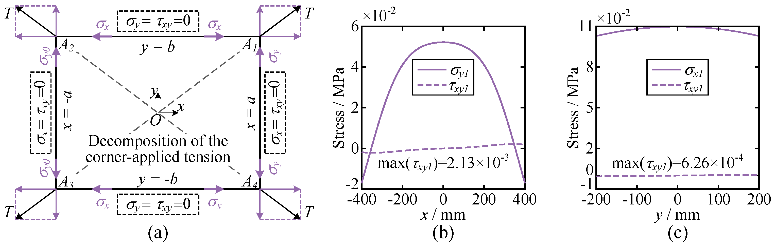
The initial prestress field is derived under an implicit infinite-domain assumption, whereby the stress field generated at each corner is unaffected by the membrane boundaries. As illustrated in Figure 2a, the corner tension in Figure 1b is resolved into the x- and y-directional components. This decomposition shows that only the tangential normal-stress component is physically applied along a membrane edge. With no externally applied shear or boundary-normal traction, the corresponding shear stress and boundary-normal stress should vanish. However, Equation (3) indicates that the initial prestress-field solution yields nonzero shear and boundary-normal stresses along the rectangular boundaries.

These two residual stress components are further examined using a representative membrane with a length of $400\mathrm{mm}$, a width of $200\mathrm{mm}$, and a thickness of $0.025\mathrm{mm}$. A corner tension of $1\mathrm{N}$ is applied to normalize the stress magnitudes and facilitate comparison of the residual-stress profiles. The boundary-normal stress ${\sigma }_{y1}$ and shear stress ${\tau }_{xy1}$ along the boundary $y=b$, together with the boundary-normal stress ${\sigma }_{x1}$ and shear stress ${\tau }_{xy1}$ along the boundary $x=a$, are calculated from Equation (3).

Figure 2b shows that, for this representative geometry, the maximum magnitude of ${\tau }_{xy1}$ along the boundary $y=b$ is only $2.13\times {10}^{-3}\mathrm{MPa}$, whereas ${\sigma }_{y1}$ is several orders of magnitude larger. A similar difference in magnitude is observed along the boundary $x=a$ in Figure 2c, where the maximum magnitude of ${\tau }_{xy1}$ is $6.26\times {10}^{-4}\mathrm{MPa}$, while ${\sigma }_{x1}$ remains several orders of magnitude larger. For the representative geometry considered here, the boundary inconsistency is therefore dominated by the residual boundary-normal stress. The subsequent formulation corrects this boundary-normal component, whereas the residual shear traction is retained as an approximation error rather than being assumed to vanish identically.

2.3. Effects of Geometry on Boundary-Normal Stress Residuals

The boundary-normal stress residual associated with the initial prestress field is therefore evaluated explicitly along the membrane edges. The prestress field is symmetric with respect to both the x- and y-axes; therefore, the right and top edges are sufficient to characterize the boundary residuals. Along the right edge, substituting $x=a$ into ${\sigma }_{x1}(x,y)$ in Equation (3) gives the boundary-normal stress residual ${\sigma }_{nx1}$. Along the top edge, substituting $y=b$ into ${\sigma }_{y1}(x,y)$ yields the corresponding boundary-normal stress residual ${\sigma }_{ny1}$.

$$\begin{array}{c}\hfill {\sigma }_{nx1}\left(y\right)={\displaystyle \sum _{i=1}^4}{\displaystyle \frac{\sqrt{2}T}{h}}{(a_i-a)}^{2}f(a,y,a_i,b_i),{\sigma }_{ny1}\left(x\right)={\displaystyle \sum _{i=1}^4}{\displaystyle \frac{\sqrt{2}T}{h}}{(b_i-b)}^{2}f(x,b,a_i,b_i)\end{array}$$

(4)

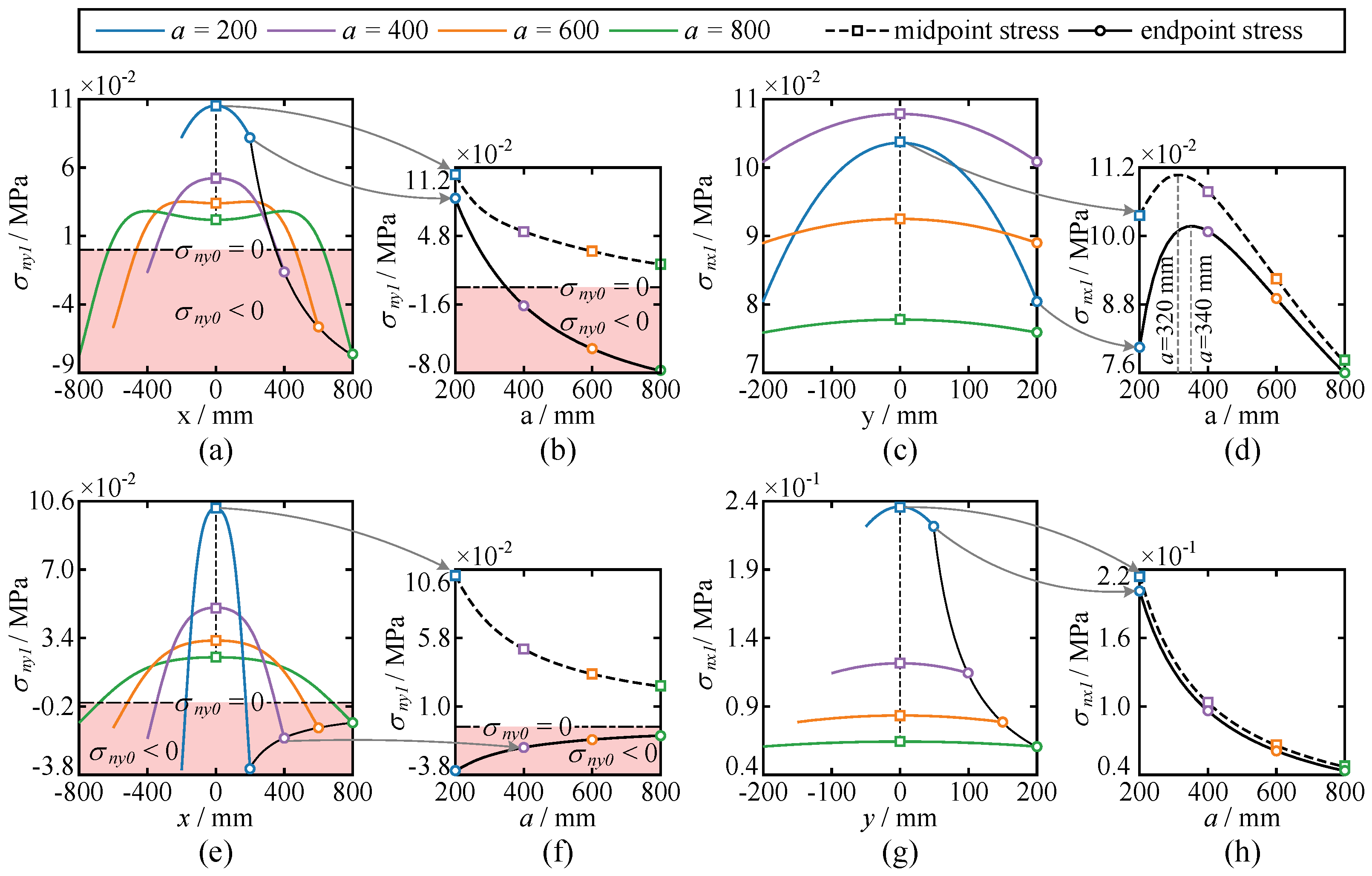
Equation (4) shows that the distribution patterns and spatial variations of ${\sigma }_{nx1}$ and ${\sigma }_{ny1}$ are primarily governed by the geometric parameters a and b, whereas T and h mainly scale the stress magnitude uniformly. The geometric dependence of these residuals is examined by evaluating Equation (4) for a series of $(a,b)$ combinations under $T=1\mathrm{N}$ and $h=0.025\mathrm{mm}$. Representative results are presented in Figure 3.

With b fixed, Figure 3a shows that the top-edge residual ${\sigma }_{ny1}$ evolves from a unimodal to a bimodal distribution as a increases. Negative values emerge near both edge ends, indicating a local reversal of the boundary-normal residual and thereby confirming violation of the zero-normal-traction condition, $F_n={\sigma }^n=0$. Figure 3b further shows that the endpoint values decrease faster than the midpoint value over $a=200$–$800\mathrm{mm}$, revealing a spatially nonuniform redistribution that produces the bimodal profile. By contrast, ${\sigma }_{nx1}$ along the right edge remains unimodal (Figure 3c) but varies nonmonotonically with a. Both midpoint and endpoint values first increase and then decrease (Figure 3d), with maxima near $a=320\mathrm{mm}$ and $a=340\mathrm{mm}$, respectively, indicating position-dependent geometric sensitivity. This contrast indicates that the endpoint regions are more sensitive to geometric variation than the midpoint.

At a fixed aspect ratio $a/b$, Figure 3e,g show that increasing the geometric scale mainly rescales the residual magnitude while preserving its spatial pattern. Thus, unimodal profiles remain unimodal, and the negative regions of ${\sigma }_{ny1}$ retain their locations and signs. As a increases, the residual peaks decrease and the distributions become flatter. Figure 3f further shows that the midpoint value of ${\sigma }_{ny1}$ decreases, whereas the negative endpoint value increases toward zero; its absolute magnitude therefore diminishes. In contrast, ${\sigma }_{nx1}$ has no negative region, and its midpoint and endpoint values both decrease monotonically with a (Figure 3h). These results indicate that, for a fixed $a/b$, geometric scaling attenuates the boundary residuals without altering their fundamental distribution characteristics or the location of the extrema.

2.4. Virtual-Load Correction and Polynomial Representation

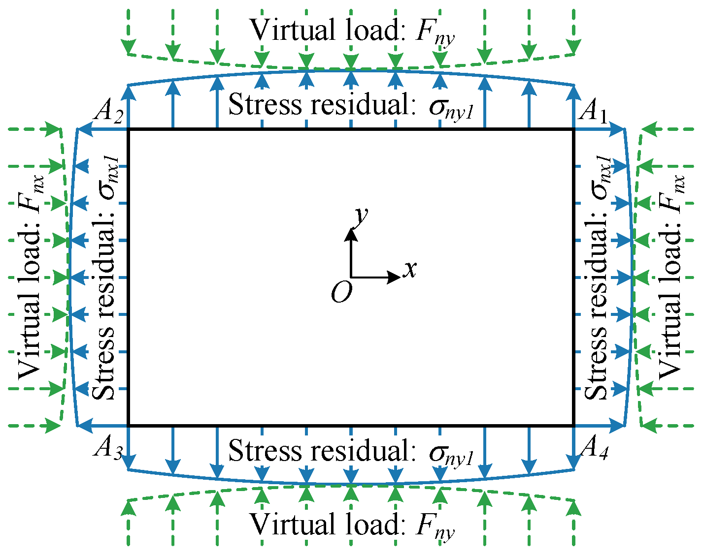
This section develops the Boundary Virtual Load Method (BVLM) by converting the boundary-normal stress residuals identified in Section 2.3 into equivalent traction-type virtual loads. As illustrated in Figure 4, the virtual loads $F_{nx}$ and $F_{ny}$ are introduced along the membrane edges to compensate for the residual boundary-normal stresses and approximate the prescribed zero-normal-traction condition. At each boundary location, the target virtual load is assigned the same magnitude as the boundary-normal stress residual generated by the initial prestress field but acts in the opposite direction. Accordingly, before polynomial approximation, the target virtual-load distributions satisfy

$$\begin{array}{c}\hfill F_{nx}+{\sigma }_{nx1}=0,F_{ny}+{\sigma }_{ny1}=0\end{array}$$

(5)

The boundary virtual loads $F_{nx}$ and $F_{ny}$ derived from Equations (4) and (5) are complex rational functions, which makes the direct construction of the corresponding Airy stress function cumbersome. They are therefore approximated by polynomial expressions to facilitate the subsequent Airy stress-function formulation. The polynomial representation enables the corrected stress field to approximate the target cancellation of the boundary-normal residuals prescribed by Equation (5). The spatial distributions of $F_{nx}$ and $F_{ny}$ inherit the characteristics of the boundary-normal stress residuals and depend strongly on the membrane geometry. This dependence is characterized by the aspect ratio $k=a/b$, and polynomial fitting is performed for $F_{nx}$ and $F_{ny}$ over different $(k,b)$ combinations.

At each $(k,b)$ pair, the discrete virtual-load distributions $F_{ny}\left(x\right)$ and $F_{nx}\left(y\right)$ are extracted along the top and right boundaries, respectively, and fitted independently with one-dimensional polynomials, where x and y denote the local boundary coordinates. Candidate polynomial degrees N are evaluated by five-fold cross-validation. In each fold, four subsets are used for training, and the remaining subset is used for validation. The mean training root-mean-square error (TR RMSE) is reported as an in-sample accuracy measure, whereas the cross-validated root-mean-square error (CV RMSE), expressed as the mean ± standard deviation over the five folds, is adopted as the primary criterion for degree selection.

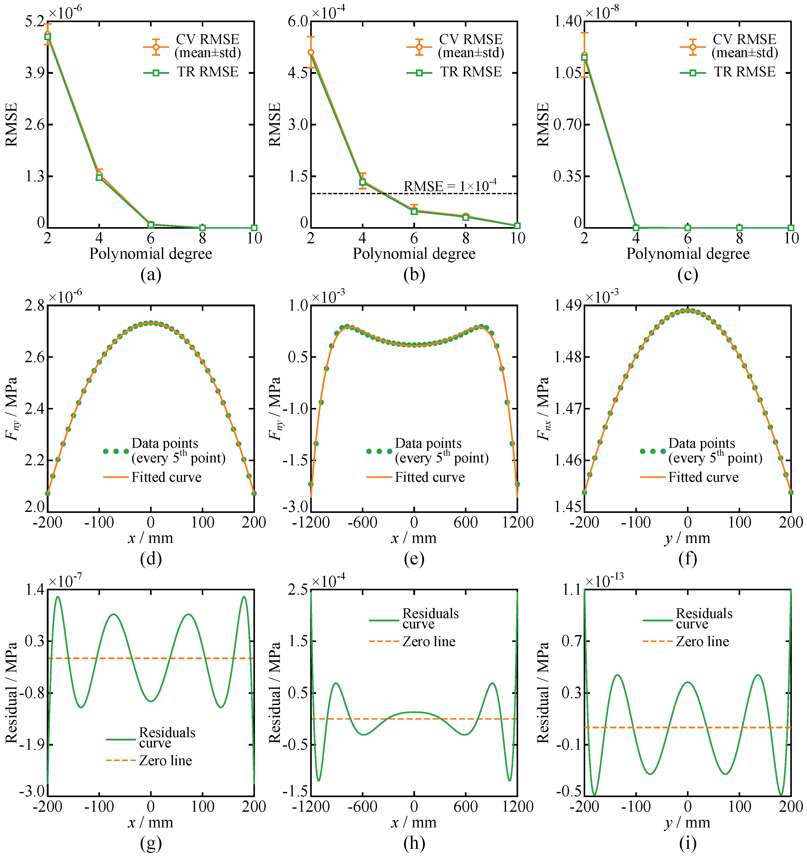
Representative fitting results are presented in Figure 5. The cases $k=1$ and $k=6$ are selected to span the aspect-ratio range considered for corner-tensioned membrane structures. At $k=1$, $F_{nx}$ and $F_{ny}$ are identical; therefore, only the result for $F_{ny}$ is shown. As shown in Figure 5a–c, both the TR RMSE and the five-fold CV RMSE decrease markedly as the polynomial degree increases from two to six, whereas higher degrees provide only limited additional improvement. Therefore, a sixth-order polynomial is selected as an appropriate compromise between fitting accuracy and model complexity. Figure 5d–f shows that the resulting polynomial curves closely reproduce the discrete virtual-load data for $F_{ny}$ at $k=1$ and $k=6$ and for $F_{nx}$ at $k=6$. The corresponding residuals in Figure 5g–i remain small and fluctuate around zero without evident systematic bias, indicating that the sixth-order approximation captures the boundary-load distributions with satisfactory accuracy.

The cross-validation procedure is used only to identify a robust polynomial order, rather than to recalibrate the order for each membrane geometry. Once the sixth-order form is fixed, the boundary residuals are evaluated analytically for a prescribed aspect ratio k and half-width b, and the corresponding polynomial coefficients are obtained by fitting these residual distributions. Coefficient expressions over the geometric range considered in this study are established by sampling k from 1 to 6 at intervals of 0.5 and b from $100\mathrm{mm}$ to $400\mathrm{mm}$ at intervals of $50\mathrm{mm}$. The resulting 77 $(k,b)$ combinations are used to characterize the dependence of the coefficients on membrane geometry.

The fitted polynomials provide an intermediate closed-form representation for constructing the Airy stress function. Owing to the even symmetry of $F_{ny}\left(x\right)$ about $x=0$ and $F_{nx}\left(y\right)$ about $y=0$, the odd-power coefficients are negligible and are omitted. Accordingly, the sixth-order virtual-load polynomials are written in the following even-power form:

$$\left\{\begin{array}{c}{F}_{ny}\left(x\right)=p_1+p_2{x}^2+p_3{x}^4+p_4{x}^6\hfill \\ F_{nx}\left(y\right)=q_1+q_2{y}^2+q_3{y}^4+q_4{y}^6\hfill \end{array}\right.$$

(6)

where $p_i$ and $q_i$ $(i=1,\dots ,4)$ denote the fitted polynomial coefficients.

At each of the 77 sampled geometries, a set of $p_i$ and $q_i$ is first obtained from the analytically evaluated boundary residuals. These discrete coefficient sets are then represented as continuous functions of k and b to obtain a directly evaluable closed-form formulation. The dependence on b is described by the scale factors $b^{-1}$, $b^{-3}$, $b^{-5}$, and $b^{-7}$ for the constant, quadratic, quartic, and sixth-order terms, respectively, whereas the remaining dependence on k is represented by rational functions. The resulting expressions are interpolation formulas valid over $1\le k\le 6$ and $100\mathrm{mm}\le b\le 400\mathrm{mm}$. Their explicit forms are given as follows:

$$\left\{\begin{array}{cc}{p}_1\hfill & =(1.374-1.345k+1.169k^2-0.253k^3)/\left[b\left(1.044+0.54k+k^2\right)\right]\hfill \\ p_2\hfill & =(-0.312+1.003k-1.639k^2+0.992k^3-0.196k^4)/\left[b^3\left(0.756-0.005k+k^2\right)\right]\hfill \\ p_3\hfill & =(0.203-2.392k+4.96k^2-4.298k^3+1.049k^4)/\left[b^5\left(0.269-0.0748k+1.0k^2\right)\right]\hfill \\ p_4\hfill & =(0.449+0.535k-0.94k^2+1.659k^3)/\left[b^7\left(23.031-52.166k+177.778k^2\right)\right]\hfill \\ q_1\hfill & =(0.315-0.444k+0.907k^2-k^3)/\left[b\left(0.578-0.564k+k^2\right)\right]\hfill \\ q_2\hfill & =(-0.001-0.143k+0.266k^2-0.236k^3+0.711k^4)/\left[b^3\left(0.065-0.18k+k^2\right)\right]\hfill \\ q_3\hfill & =(-0.049+0.169k-0.279k^2+0.205k^3-0.053k^4)/\left[b^5\left(0.028-0.043k+k^2\right)\right]\hfill \\ q_4\hfill & =(0.032-0.099k+0.136k^2-0.111k^3+0.178k^4)/\left[b^7\left(0.036-0.011k+k^2\right)\right]\hfill \end{array}\right.$$

(7)

2.5. Airy Stress-Function Solution

The stress components induced by the Airy stress function are expressed as

$${\sigma }_{x2}={\displaystyle \frac{{\partial }^2{\mathsf{\Phi }}_2}{\partial y^2}},{\sigma }_{y2}={\displaystyle \frac{{\partial }^2{\mathsf{\Phi }}_2}{\partial x^2}},{\tau }_{xy2}=-{\displaystyle \frac{{\partial }^2{\mathsf{\Phi }}_2}{\partial x\partial y}}$$

(8)

The boundary virtual loads in Equation (6) are represented by sixth-degree polynomials. The stress components follow from second-order differentiation of the Airy stress function, which reduces the polynomial degree by two. This relation requires the Airy stress function ${\mathsf{\Phi }}_2(x,y)$ associated with the boundary virtual loads to contain terms up to the eighth degree. Quadratic terms are also included in ${\mathsf{\Phi }}_2$ so that constant terms can be retained in the resulting stress components.

$${\mathsf{\Phi }}_2(x,y)=L_8(x,y)+L_6(x,y)+L_2(x,y)$$

(9)

The Airy stress function ${\mathsf{\Phi }}_2(x,y)$ is constructed as an even function with respect to both x and y, consistent with the even symmetry of the top-boundary virtual load $F_{ny}\left(x\right)$ about $x=0$ and that of the right-boundary virtual load $F_{nx}\left(y\right)$ about $y=0$. Only even-power terms are therefore retained in the polynomial representation.

$$\left\{\begin{array}{c}{L}_8(x,y)=u_8{x}^8+u_6{x}^6{y}^2+u_4{x}^4{y}^4+u_2{x}^2{y}^6+u_0{y}^8\hfill \\ L_6(x,y)=v_6{x}^6+v_4{x}^4{y}^2+v_2{x}^2{y}^4+v_0{y}^6\hfill \\ L_2(x,y)=w_2{x}^2+w_0{y}^2\hfill \end{array}\right.$$

(10)

where $u_i$, $v_i$, and $w_i$ are undetermined coefficients.

Substituting Equations (9) and (10) into Equation (8) yields the stress components induced by the boundary virtual loads.

$$\left\{\begin{array}{c}{\sigma }_{x2}={\displaystyle \frac{{\partial }^2{\mathsf{\Phi }}_2}{\partial y^2}}=\left(\begin{array}{c}56u_0{y}^6+30u_2{x}^2{y}^4+12u_4{x}^4{y}^2+2u_6{x}^6\\ +30v_0{y}^4+12v_2{x}^2{y}^2+2v_4{x}^4+2w_0\end{array}\right)\hfill \\ {\sigma }_{y2}={\displaystyle \frac{{\partial }^2{\mathsf{\Phi }}_2}{\partial x^2}}=\left(\begin{array}{c}56u_8{x}^6+30u_6{x}^4{y}^2+12u_4{x}^2{y}^4+2u_2{y}^6\\ +30v_6{x}^4+12v_4{x}^2{y}^2+2v_2{y}^4+2w_2\end{array}\right)\hfill \\ {\tau }_{xy2}=-{\displaystyle \frac{{\partial }^2{\mathsf{\Phi }}_2}{\partial x\partial y}}=-\left(\begin{array}{c}12u_6{x}^{5}y+16u_4{x}^3{y}^3+12u_{2}x{y}^5+8v_4{x}^{3}y+8v_{2}x{y}^3\end{array}\right)\hfill \end{array}\right.$$

(11)

Equation (11) shows that ${\tau }_{xy2}$ is odd with respect to both x and y. Consequently, ${\tau }_{xy2}=0$ is automatically satisfied along $x=0$ and $y=0$, which is consistent with the symmetry conditions of the membrane. In a plane linear-elastic problem without body forces, the Airy stress function must also satisfy the biharmonic equation.

$${\nabla }^4{\mathsf{\Phi }}_2(x,y)=0,{\nabla }^4={\left({\nabla }^2\right)}^2$$

(12)

Substituting Equations (9) and (10) into the biharmonic condition in Equation (12) gives

$$\begin{array}{cc}\hfill {\nabla }^4{\mathsf{\Phi }}_2=& \left(1680u_8+120u_6+24u_4\right)x^4+\left(360u_6+288u_4+360u_2\right)x^2{y}^2\hfill \\ \hfill & +\left(24u_4+120u_2+1680u_0\right)y^4+\left(360v_6+48v_4+24v_2\right)x^2\hfill \\ \hfill & +\left(24v_4+48v_2+360v_0\right)y^2=0.\hfill \end{array}$$

(13)

The linear independence of the monomials $x^4$, $x^2{y}^2$, $y^4$, $x^2$, and $y^2$ requires the coefficient of each monomial to vanish independently. This requirement yields the following constraints on the coefficients:

$$\left\{\begin{array}{c}24u_4+120u_6+1680u_8=0\hfill \\ 24u_4+120u_2+1680u_0=0\hfill \\ 360u_2+288u_4+360u_6=0\hfill \\ 24v_2+48v_4+360v_6=0\hfill \\ 24v_4+48v_2+360v_0=0\hfill \end{array}\right.$$

(14)

The boundary conditions additionally require ${\sigma }_{y2}$ to match the virtual load $F_{ny}\left(x\right)$ on the top and bottom boundaries, $y=\pm b$, and ${\sigma }_{x2}$ to match the virtual load $F_{nx}\left(y\right)$ on the right and left boundaries, with $x=\pm a$. Equating the corresponding polynomial terms in Equations (6) and (11) along $y=\pm b$ and $x=\pm a$ yields

$$\begin{array}{c}{\sigma }_{y2}{|}_{y=\pm b}=F_{ny}\left(x\right)\Rightarrow \left\{\begin{array}{cc}2(u_2{b}^6+v_2{b}^4+w_2)=p_1,\hfill & 12(u_4{b}^4+v_4{b}^2)=p_2\hfill \\ 30(u_6{b}^2+v_6)=p_3,\hfill & 56u_8=p_4\hfill \end{array}\right.\\ {\sigma }_{x2}{|}_{x=\pm a}=F_{nx}\left(y\right)\Rightarrow \left\{\begin{array}{cc}2(u_6{a}^6+v_4{a}^4+w_0)=q_1,\hfill & 12(u_4{a}^4+v_2{a}^2)=q_2\hfill \\ 30(u_2{a}^2+v_0)=q_3,\hfill & 56u_0=q_4\hfill \end{array}\right.\end{array}$$

(15)

Solving the coupled system of Equations (14) and (15) yields the polynomial coefficients of ${\mathsf{\Phi }}_2(x,y)$:

$$\left\{\begin{array}{c}{u}_0=q_4/56\hfill \\ u_2=-(p_4+3q_4)/8\hfill \\ u_4=5(p_4+q_4)/8\hfill \\ u_6=-(q_4+3p_4)/8\hfill \\ u_8=p_4/56\hfill \\ v_0=a^2{p}_4/8+3a^2{q}_4/8+q_3/30\hfill \\ v_2=(-15a^4{p}_4-15a^4{q}_4+2q_2)/24a^2\hfill \\ v_4=(-15b^4{p}_4-15b^4{q}_4+2p_2)/24b^2\hfill \\ v_6=3b^2{p}_4/8+b^2{q}_4/8+p_3/30\hfill \\ w_0=(9a^6{b}^2{p}_4+3a^6{b}^2{q}_4+15a^4{b}^4{q}_4+15a^4{b}^4{p}_4-2a^4{p}_2+12b^2{q}_1)/24b^2\hfill \\ w_2=(9a^2{b}^6{q}_4+3a^2{b}^6{p}_4+15a^4{b}^4{q}_4+15a^4{b}^4{p}_4-2a^4{q}_2+12b^2{p}_1)/24a^2\hfill \end{array}\right.$$

(16)

Substituting Equation (16) into Equation (11) gives the stress components induced by the polynomially approximated boundary virtual loads. Superposition of these correction-induced stress components with the initial prestress field in Equation (3) yields the final BVLM semi-analytical prestress representation.

$$\left\{\begin{array}{c}{\sigma }_x={\sigma }_{x1}+{\sigma }_{x2}\hfill \\ {\sigma }_y={\sigma }_{y1}+{\sigma }_{y2}\hfill \\ {\tau }_{xy}={\tau }_{xy1}+{\tau }_{xy2}\hfill \end{array}\right.$$

(17)

3. Prestress-Field Characteristics and Finite Element Validation

BVLM is applied in this section to examine three representative membrane configurations. The preceding analysis indicates that the in-plane stress distribution is primarily governed by the aspect ratio, whereas uniform scaling of both length and width alters only the stress magnitude and leaves the distribution pattern unchanged. The case-study geometries are therefore selected to match the experimental specimens used in the subsequent modal analysis.

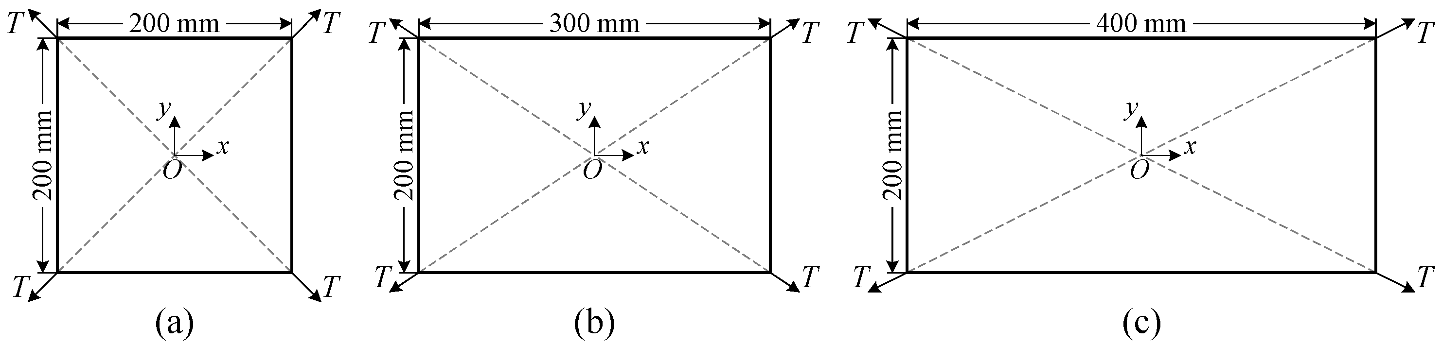
As shown in Figure 6, the membrane lengths are set to $200\mathrm{mm}$, $300\mathrm{mm}$, and $400\mathrm{mm}$, respectively, with a uniform width of $200\mathrm{mm}$ and a thickness of $0.025\mathrm{mm}$. The stress components and their directions are defined in a Cartesian coordinate system centered at the membrane centroid. Each of the four corners is subjected to a diagonal tensile load of $10\mathrm{N}$. Accordingly, the validation cases considered in this section cover membrane aspect ratios from 1 to 2, with lengths of 200–$400\mathrm{mm}$, a fixed width of $200\mathrm{mm}$, a thickness of $0.025\mathrm{mm}$, and a corner tensile load of $10\mathrm{N}$.

3.1. BVLM-Predicted Prestress Distribution Characteristics

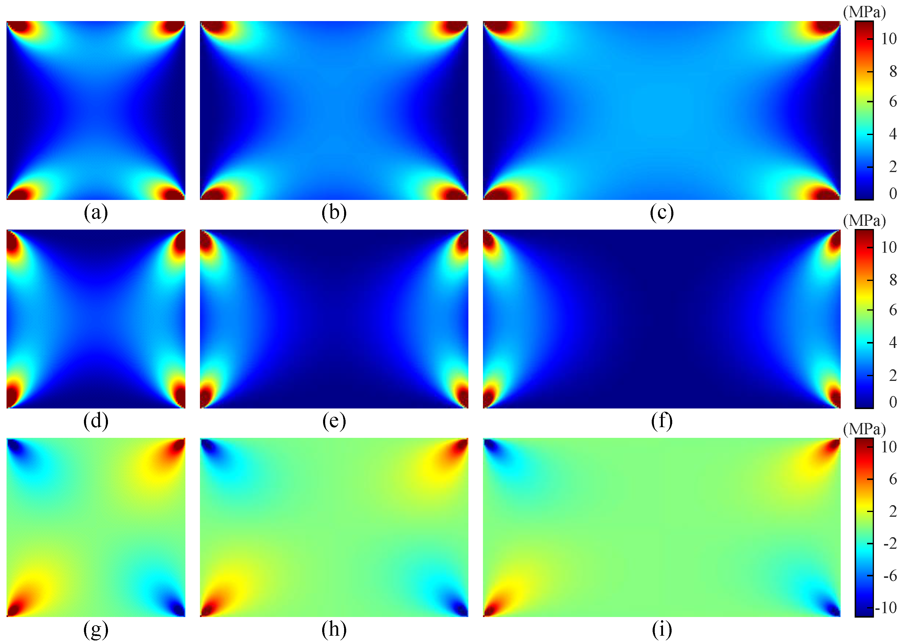
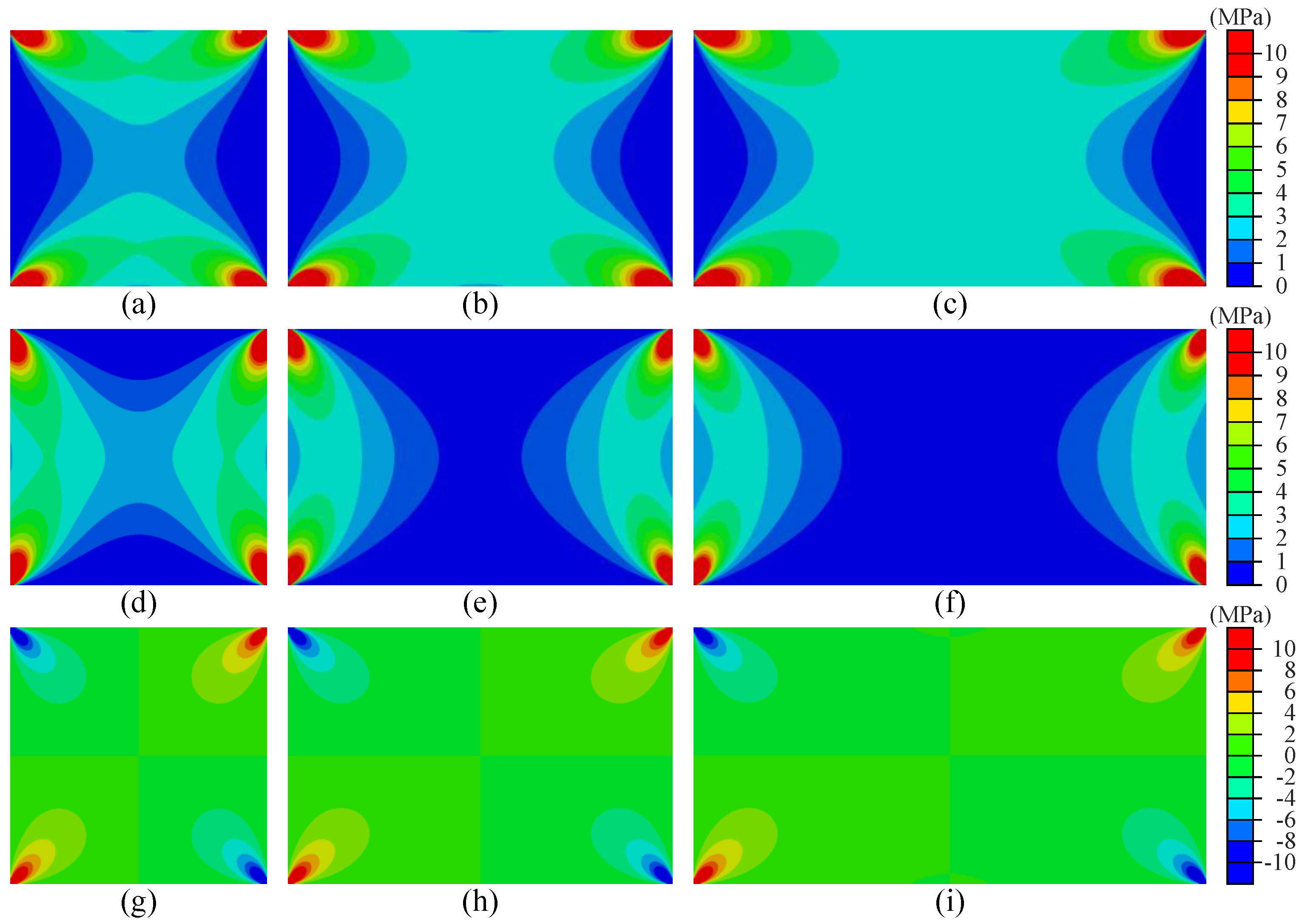
The prestress fields for the three cases are computed using BVLM and visualized as contour plots. Figure 7 presents the distributions of the three stress components: subfigures (a)–(c) show the normal stress ${\sigma }_x$, subfigures (d)–(f) show the normal stress ${\sigma }_y$, and subfigures (g)–(i) show the shear stress ${\tau }_{xy}$.

In Case I (Figure 7a), the normal stress ${\sigma }_x$ is strongly concentrated around the corners and decays along the diagonal paths toward the membrane interior. The central region remains at comparatively low prestress levels, revealing pronounced localization of the corner-induced normal stress. In Case II (Figure 7b), the corner prestress-concentration zones extend farther into the membrane, and the magnitude of ${\sigma }_x$ in the central region increases appreciably. In Case III (Figure 7c), the overall prestress field becomes smoother, with a further reduction in the stress gradient. The ${\sigma }_x$ component is redistributed more uniformly along the diagonal paths, producing an “X”-shaped moderate-prestress region near the membrane center. This evolution indicates that an increasing aspect ratio promotes the transfer of corner-induced ${\sigma }_x$ from the loaded corners toward the membrane interior.

The ${\sigma }_y$ distribution in Case I (Figure 7d) closely resembles the ${\sigma }_x$ distribution in Figure 7a, which is consistent with the square membrane geometry. Both stress components show a localized pattern, with high stresses concentrated near the corners and low stresses in the central region. As the membrane length increases (Figure 7e,f), ${\sigma }_y$ evolves into a boundary-dominated prestress field. In Figure 7e, ${\sigma }_y$ is mainly concentrated along the lateral edges and corner regions, whereas the central region approaches a nearly prestress-free state. This behavior indicates that ${\sigma }_y$ is largely confined to the boundary vicinity and is not effectively transferred into the membrane interior. This tendency becomes more pronounced in Case III (Figure 7f), where the central low-prestress region expands further and ${\sigma }_y$ is almost completely restricted to the edge regions. Overall, a larger aspect ratio weakens the interior transmission of ${\sigma }_y$ and makes its distribution increasingly governed by the boundary loading paths.

Across all cases, the shear stress ${\tau }_{xy}$ exhibits a distinctly boundary-dominated distribution, with large magnitudes localized primarily near the corners. In Case I (Figure 7g), four localized high-shear-stress regions appear at the corners, forming a symmetric fan-shaped pattern along the diagonal directions. Adjacent shear-stress regions have opposite signs, with positive (red) and negative (blue) regions appearing in pairs. As the membrane length increases (Figure 7h,i), the high-shear-stress zones contract and become confined to smaller corner regions. Although the polarity pattern is preserved, its spatial extent is markedly reduced relative to that in Case I, and the shear stress in the central region approaches zero. This behavior indicates that the interior transmission of ${\tau }_{xy}$ is substantially weakened as the aspect ratio increases.

3.2. Finite Element Verification of the BVLM-Predicted Prestress Field

3.2.1. Mesh-Independence Verification

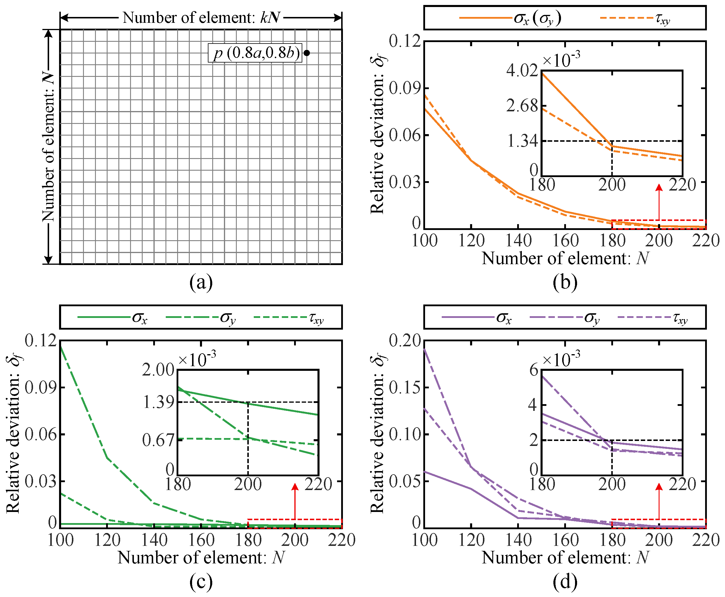
Mesh-density effects are systematically investigated with structured square elements, as illustrated in Figure 8a. The short side is discretized into N elements, whereas the long side is discretized into $kN$ elements, so that a uniform element size is maintained throughout the membrane domain. A stress-monitoring point is defined at $p(0.8a,0.8b)$. The initial mesh density is set to $N_0=20$, and N is increased by 20 elements at each refinement step. The stress components at the monitoring point are extracted and compared across different mesh densities to assess mesh-refinement convergence. The relative deviation ${\delta }_f$ is defined as

$${\delta }_f={\displaystyle \frac{|\sigma -{\sigma }_{last}|}{{\sigma }_{last}}}$$

(18)

where $\sigma$ and ${\sigma }_{last}$ denote the stress values at point p obtained from the current and previous mesh densities, respectively. The mesh is regarded as sufficiently refined once the relative deviation ${\delta }_f$ falls below and remains under $0.2\%$.

Figure 8b–d present the mesh-convergence behavior of the three stress components at point p under different mesh densities, as quantified by the relative deviation ${\delta }_f$. As the mesh is progressively refined, the relative-deviation curves decrease and approach stable values in all three cases, indicating satisfactory numerical convergence. At $N\ge 200$, the relative deviations of the stress components at point p remain below $0.14\%$ for Case I and Case II (Figure 8b,c) and below $0.2\%$ for Case III (Figure 8d). Considering both computational accuracy and efficiency, a mesh density of $N=200$ is adopted for all subsequent finite element analyses.

3.2.2. Finite Element Verification of Prestress-Field Distributions

The prestress contour maps computed from the finite element simulations are presented in Figure 9. The material properties adopted in the finite element model are listed in

Table 1. Material and surrounding-air parameters used in the numerical and experimental analyses.

Parameter	Symbol	Value	Unit
Young’s modulus of the membrane	E	2551	$\mathrm{MPa}$
Poisson’s ratio of the membrane	$\nu$	0.34	–
Membrane density	${\rho }_m$	1430	$\mathrm{kg}/{\mathrm{m}}^3$
Air density	${\rho }_{\mathrm{air}}$	1.225	$\mathrm{kg}/{\mathrm{m}}^3$

. The finite element reference solutions are obtained from geometrically nonlinear membrane analyses that account for deformation-induced updates of the membrane geometry during loading. Comparison with these reference solutions therefore is also used to assess the fixed-geometry approximation adopted in the BVLM formulation under the geometric, material, and loading conditions considered in this study. The reliability of the BVLM predictions is evaluated by directly comparing the finite element prestress distributions with the BVLM-predicted fields shown in Figure 7.

Overall, the finite element results show prestress-distribution patterns that agree well with those predicted by BVLM. Specifically, as the membrane length increases, ${\sigma }_x$ remains concentrated near the corners and gradually develops an “X”-shaped moderate-prestress region around the membrane center; ${\sigma }_y$ is primarily localized along the edges and decreases to nearly zero in the central region, accompanied by an expansion of the central low-stress zone; and ${\tau }_{xy}$ consistently exhibits a highly symmetric fan-shaped pattern about the x and y axes. This qualitative agreement indicates that BVLM captures the principal spatial characteristics of the corner-induced prestress field for the examined membrane configurations.

3.2.3. Comparison of BVLM and FEM Stress Components Along Representative Cross Sections

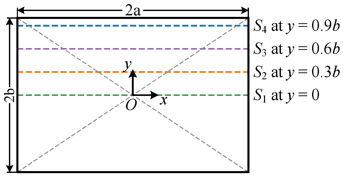
BVLM and finite element results are quantitatively compared using stress profiles extracted along four equally spaced cross-sections ($S_1$, $S_2$, $S_3$, and $S_4$) extending from the membrane center to the boundary, as illustrated in Figure 10.

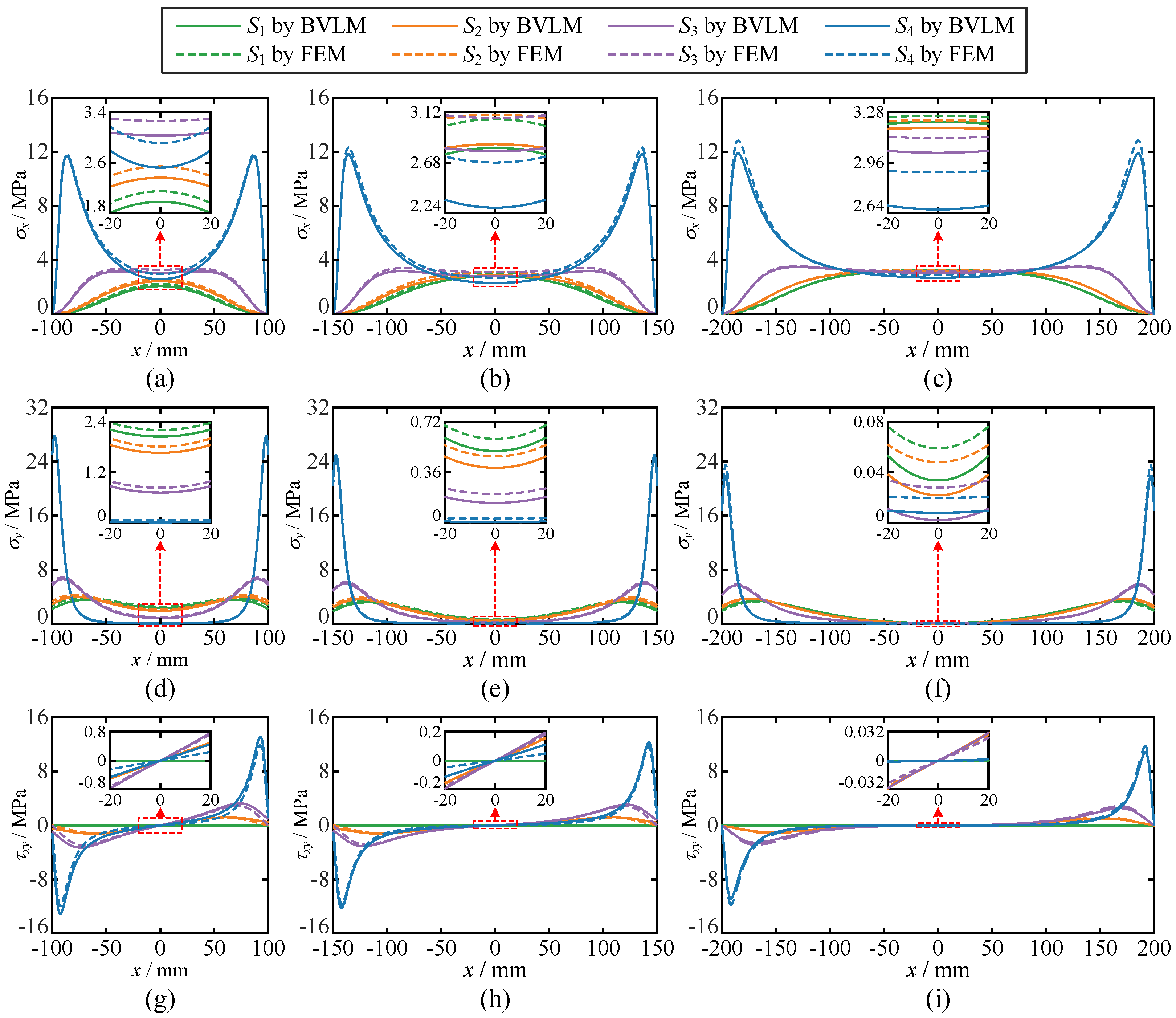
Stress profiles along cross-sections $S_1$–$S_4$ are extracted for all three cases from the BVLM-predicted fields (Figure 7) and the finite element results (Figure 9), as shown in Figure 11. Along these cross-sections, the two methods show generally consistent variation trends and reasonable quantitative agreement. Near the corners, both approaches capture the corner-stretching-induced stress concentrations, with close agreement in peak locations, peak magnitudes, and local gradients. From the boundary toward the membrane center, the stress profiles become increasingly smooth and uniform. These results indicate that BVLM can reproduce the stress variations obtained from finite element simulations with reasonable accuracy. Component-wise comparisons of ${\sigma }_x$, ${\sigma }_y$, and ${\tau }_{xy}$ are presented below.

Regarding ${\sigma }_x$, Case I (Figure 11a) shows close agreement between the BVLM predictions and FEM results, especially near the ends of each cross-section. At the peak along $S_4$, the two results are nearly identical, with peak stresses of 11.7 and $11.8\mathrm{MPa}$, corresponding to a difference of only $0.1\mathrm{MPa}$ (0.85%). The main discrepancies occur in the central low-stress regions, where the deviations along $S_1$–$S_4$ increase from $0.16$–$0.38\mathrm{MPa}$ in Case I to $0.24$–$0.44\mathrm{MPa}$ in Case III. The maximum deviation therefore increases by 15.8%, indicating a slight reduction in BVLM accuracy in the membrane interior as the aspect ratio increases. Near the peaks of $S_4$, BVLM shows a mild underestimation relative to FEM in the longer membranes, with the peak difference increasing from $0.56\mathrm{MPa}$ (4.10%) in Case II to $1.06\mathrm{MPa}$ (7.54%) in Case III.

Regarding ${\sigma }_y$ (Figure 11d–f), the BVLM and FEM results show peak differences of $0.24$, $0.20$, and $1.68\mathrm{MPa}$ near the two ends of cross-section $S_4$ in Cases I–III, respectively. In Case I and Case II (Figure 11d,e), the two methods show close agreement, with relative errors below 1%. In Case III (Figure 11f), the discrepancy increases, with the relative error reaching 7.31%. At the cross-section centers, the largest deviation among $S_1$–$S_4$ occurs at $S_1$, with values of 0.16, 0.08, and 0.06$\mathrm{MPa}$ for Cases I–III, respectively. The smallest deviation occurs at $S_4$, with corresponding values of 0.04, 0.01, and 0.02$\mathrm{MPa}$. The decreasing central magnitude of ${\sigma }_y$ in longer membranes reduces the BVLM–FEM discrepancy in the membrane interior.

Regarding ${\tau }_{xy}$ (Figure 11g–i), both BVLM and FEM capture the stress concentrations near the edges of each cross-section and the gradual stress variation in the central region. Along cross-section $S_4$, which is located close to the corner region, BVLM predicts peak shear stresses of 13.10, 12.28, and 10.82 $\mathrm{MPa}$ for Cases I–III, respectively, whereas FEM gives corresponding values of 11.84, 11.70, and 11.62 $\mathrm{MPa}$. In Case I and Case II, BVLM slightly overestimates the FEM peak stresses by 10.6% and 4.95%, respectively, whereas Case III shows an underestimation of 6.88%. This behavior indicates a modest dependence of BVLM accuracy on the membrane aspect ratio. Both methods also capture the polarity reversal near cross-sections $S_2$–$S_3$, where the shear stress changes from negative to positive, demonstrating good agreement in the predicted shear-stress transfer and sign-transition behavior.

Overall, the agreement between the BVLM predictions and the geometrically nonlinear FEM results for the three membrane configurations indicates that the fixed-geometry approximation does not introduce a dominant error in the Cartesian prestress components within the range of geometric and loading conditions investigated in this study.

3.2.4. Computational Efficiency Comparison Between BVLM and FEM

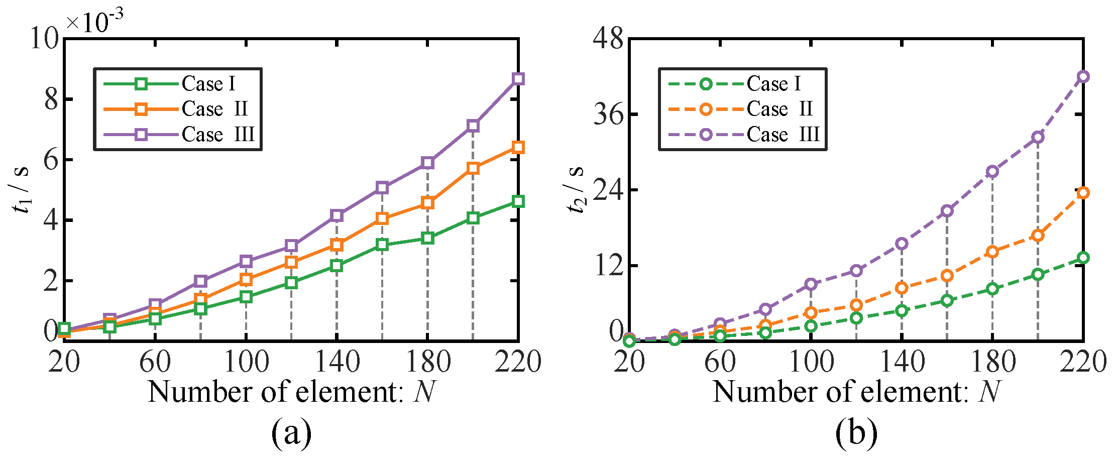
The computational efficiency of BVLM relative to FEM is evaluated by comparing the computation times for the three cases under different values of N. All simulations are conducted on a Lenovo laptop (Lenovo Group Ltd., Beijing, China) equipped with an AMD Ryzen 9 7945HX CPU, 32 GB RAM, and an NVIDIA RTX 4060 GPU, running Windows 11. The reported FEM computation time is taken directly from the “Total Time” recorded in the solver system file and spans the complete interval from job submission to result-file generation. The reported BVLM time includes evaluation of all three Cartesian stress components, ${\sigma }_x$, ${\sigma }_y$, and ${\tau }_{xy}$, over the entire membrane domain at the same spatial resolution as the corresponding FEM analysis. Thus, at each value of N, BVLM and FEM are compared on an equivalent spatial-resolution basis. As shown in Figure 12, the computation times of BVLM and FEM are denoted by $t_1$ and $t_2$, respectively. Under the computational settings and membrane cases considered, BVLM requires substantially shorter evaluation times than FEM, indicating a lower computational cost for the examined analyses. At $N=200$ for Case III, BVLM requires only $7.1\times {10}^{-3}\mathrm{s}$, whereas FEM requires $32.5\mathrm{s}$. The FEM computation time is therefore approximately 4577 times that of BVLM. This speedup should be interpreted under the above hardware, spatial-resolution, and timing definitions rather than as a universal performance ratio between BVLM and FEM.

This reduction in evaluation time facilitates rapid design iteration, large-scale parametric studies, sensitivity and trade-off analyses during early-stage design, and high-resolution evaluation of large membrane structures with substantially reduced computational burden. Consequently, BVLM is well suited to rapid screening and optimization tasks, whereas FEM can be reserved for final verification and localized refinement.

4. Modal Analysis and Experimental Assessment

4.1. Prestressed Membrane Vibration Model

The BVLM-predicted prestress field is introduced into a free-vibration model that incorporates the surrounding air medium. The resulting modal characteristics provide experimentally accessible quantities for indirectly assessing the dynamic consistency of the predicted prestress distribution. The rectangular membrane is discretized using planar isoparametric quadrilateral elements [33]. Using a four-node bilinear quadrilateral element, the shape-function vector is defined as $\mathit{N}=[N_1,N_2,N_3,N_4]$, where

$$\begin{array}{cccc}\hfill N_1& ={\displaystyle \frac{1}{4}}(1-\xi )(1-\eta ),\hfill & \hfill N_2& ={\displaystyle \frac{1}{4}}(1+\xi )(1-\eta ),\hfill \\ \hfill N_3& ={\displaystyle \frac{1}{4}}(1+\xi )(1+\eta ),\hfill & \hfill N_4& ={\displaystyle \frac{1}{4}}(1-\xi )(1+\eta )\hfill \end{array}$$

in which $\xi$ and $\eta$ denote the natural coordinates of the element. With three displacement components, the corresponding interpolation matrix can be expressed as ${\mathit{I}}_3\otimes \mathit{N}$, where ${\mathit{I}}_3$ is the $3\times 3$ identity matrix and ⊗ denotes the Kronecker product. The corresponding element mass matrix is expressed as

$${\mathit{M}}_e={\displaystyle \frac{{\rho }_{m}h}{2}}\left[\begin{array}{ccc}\int \int {\mathit{N}}^T\mathit{N}dxdy& 0& 0\\ 0& \int \int {\mathit{N}}^T\mathit{N}dxdy& 0\\ 0& 0& \int \int {\mathit{N}}^T\mathit{N}dxdy\end{array}\right]$$

(19)

where ${\rho }_m$ denotes the membrane density and h the membrane thickness.

Let the initial prestress state in the membrane be ${\sigma }_0=[{\sigma }_{x0},{\sigma }_{y0},{\tau }_{xy0}]$. The corresponding element stiffness matrix is written as

$${\mathit{K}}_e=\left[\begin{array}{cc}{\mathit{K}}_m& 0\\ 0& {\mathit{K}}_g\end{array}\right]$$

(20)

where ${\mathit{K}}_m$ and ${\mathit{K}}_g$ denote the material and geometric stiffness matrices, respectively. The matrices $\mathit{B}$ and $\mathit{C}$ contain the spatial derivatives of the element shape functions in the x- and y-directions, respectively, and are defined as

$$\begin{array}{cc}\hfill \mathit{B}& =\left[\begin{array}{cccc}{\displaystyle \frac{\partial N_1}{\partial x}}& {\displaystyle \frac{\partial N_2}{\partial x}}& {\displaystyle \frac{\partial N_3}{\partial x}}& {\displaystyle \frac{\partial N_4}{\partial x}}\end{array}\right],\hfill \\ \hfill \mathit{C}& =\left[\begin{array}{cccc}{\displaystyle \frac{\partial N_1}{\partial y}}& {\displaystyle \frac{\partial N_2}{\partial y}}& {\displaystyle \frac{\partial N_3}{\partial y}}& {\displaystyle \frac{\partial N_4}{\partial y}}\end{array}\right].\hfill \end{array}$$

The derivatives with respect to the physical coordinates $(x,y)$ are obtained from those in the natural coordinates $(\xi ,\eta )$ through the standard isoparametric coordinate transformation. Their explicit expressions are given as follows [33]:

$$\left\{\begin{array}{c}{\displaystyle {\mathit{K}}_m=\left[\begin{array}{cc}{\displaystyle \int \int \left(\frac{Eh}{1-{\mu }^2}{\mathit{B}}^T\mathit{B}+\frac{Eh}{2(1+\mu )}{\mathit{C}}^T\mathit{C}\right)dxdy}& {\displaystyle \int \int \left(\frac{Eh\mu }{1-{\mu }^2}{\mathit{B}}^T\mathit{C}+\frac{Eh}{2(1+\mu )}{\mathit{C}}^T\mathit{B}\right)dxdy}\\ {\displaystyle \int \int \left(\frac{Eh\mu }{1-{\mu }^2}{\mathit{C}}^T\mathit{B}+\frac{Eh}{2(1+\mu )}{\mathit{B}}^T\mathit{C}\right)dxdy}& {\displaystyle \int \int \left(\frac{Eh}{1-{\mu }^2}{\mathit{C}}^T\mathit{C}+\frac{Eh}{2(1+\mu )}{\mathit{B}}^T\mathit{B}\right)dxdy}\end{array}\right]}\hfill \\ {\displaystyle {\mathit{K}}_g=\int \int h\left({\sigma }_{x0}{\mathit{B}}^T\mathit{B}+{\sigma }_{y0}{\mathit{C}}^T\mathit{C}+{\tau }_{xy0}{\mathit{B}}^T\mathit{C}+{\tau }_{xy0}{\mathit{C}}^T\mathit{B}\right)dxdy}\hfill \end{array}\right.$$

(21)

Practical constraints make modal testing of membranes under a vacuum difficult; consequently, ground-based experiments are typically conducted in air. The free-vibration equation of a membrane in an atmospheric environment is expressed as [28]

$$-{\omega }_k^2(1+\alpha )\mathit{M}{\mathsf{\Phi }}_k+{\mathit{K}}^T{\mathsf{\Phi }}_k=0$$

(22)

where $\alpha$ denotes the added-mass ratio, defined as the ratio of the effective mass of the surrounding air to the mass of the vibrating membrane. Minami [34] analyzed membrane vibration in air and showed that $\alpha$ is independent of the oscillation period and amplitude. The study further showed that the equivalent uniform air layer representing the membrane added mass has a height equal to 68% of the membrane length, consistent with results obtained using the source-distribution Green’s function approach. Minami expressed the added-mass ratio as

$$\alpha =0.68{\rho }_{\mathrm{air}}{l}_m/\left(h{\rho }_m\right)$$

(23)

where ${\rho }_{\mathrm{air}}$ denotes the air density, $l_m=2a$ is the membrane length, and ${\rho }_m$ is the membrane density.

4.2. Experimental Setup and Modal Testing Results

Experimental modal tests are conducted on prestressed membrane specimens to assess the proposed modeling and solution framework. The material properties, geometric dimensions, and boundary conditions used in the experiments closely match those specified in the theoretical model, enabling direct and repeatable comparisons.

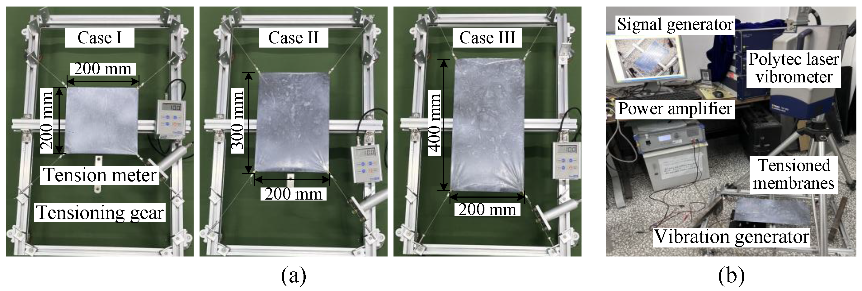
All membrane specimens are fabricated from a polyimide membrane with a thickness of $0.025\mathrm{mm}$. The specimen geometries correspond to those examined in the preceding analyses, $200\mathrm{mm}\times 200\mathrm{mm}$ (Case I), $300\mathrm{mm}\times 200\mathrm{mm}$ (Case II), and $400\mathrm{mm}\times 200\mathrm{mm}$ (Case III), as shown in Figure 13a. A diagonal pretension of $10\mathrm{N}$ is applied at each membrane corner using a tensioning device in conjunction with a calibrated tension gauge, thereby establishing a stable and controllable initial prestress field. This loading configuration reproduces the corner-tensioned boundary conditions prescribed in the theoretical analysis and enables direct comparison between the predicted and measured modal characteristics.

Modal testing is performed using a Polytec laser Doppler vibrometer (LDV) system, as illustrated in Figure 13b. A thin diffuse-reflective coating is applied to the membrane surface to reduce specular reflections and enhance measurement quality. An electromagnetic shaker provides excitation over a frequency range of 0–$100\mathrm{Hz}$, while the scanning vibrometer records the full-field vibration response. The measured frequency response functions (FRFs) are subsequently processed to identify the experimental modal parameters. These identified modal parameters are compared with the theoretical predictions to evaluate the accuracy and applicability of the BVLM-based model across rectangular membranes with different geometries.

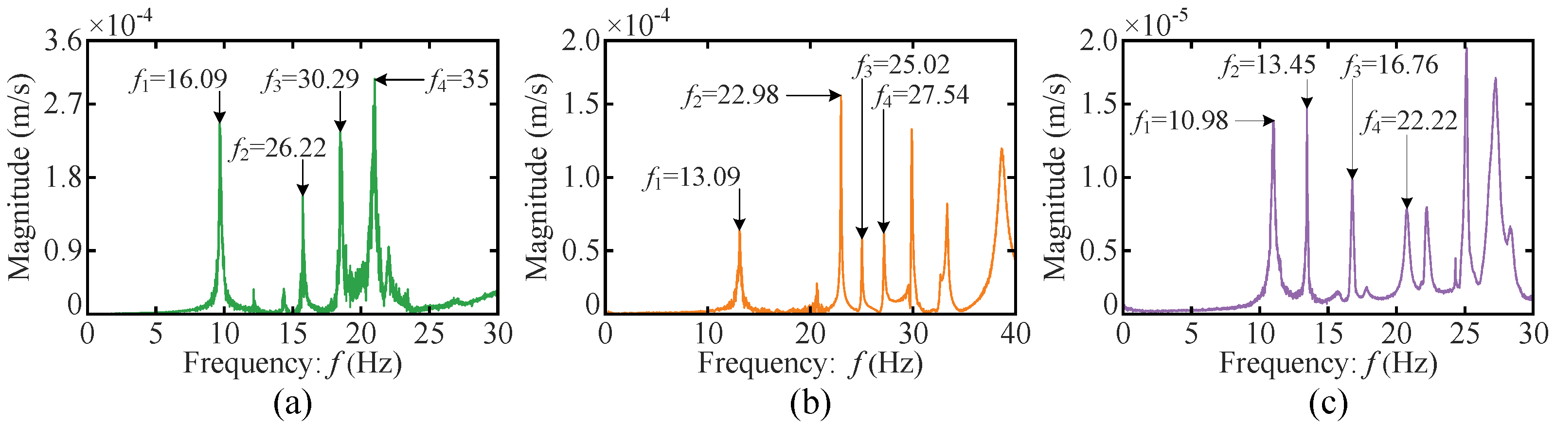
Frequency response curves are obtained from modal tests of the three membrane specimens, as shown in Figure 14. All FRFs exhibit clear, well-separated resonance peaks, demonstrating well-defined modal characteristics. In Case I (Figure 14a), the first four resonance peaks occur at 16.09, 26.22, 30.29, and $35.00\mathrm{Hz}$, and the maximum velocity amplitude reaches $3.01\times {10}^{-4}\mathrm{m}/\mathrm{s}$. Increasing the membrane length shifts the resonance peaks progressively toward lower frequencies. In Case II (Figure 14b), the first four peaks occur at 13.09, 22.98, 25.02, and $27.54\mathrm{Hz}$, with a maximum velocity amplitude of $1.60\times {10}^{-4}\mathrm{m}/\mathrm{s}$. The lower modal frequencies reflect the increased structural compliance associated with the larger span and reduced effective stiffness. In Case III (Figure 14c), the first four resonance frequencies decrease further to $10.98$–$22.22\mathrm{Hz}$. The maximum velocity amplitude decreases to $1.51\times {10}^{-5}\mathrm{m}/\mathrm{s}$, more than one order of magnitude below the maxima measured in Cases I and II, indicating a substantially attenuated dynamic response under the same excitation condition.

This monotonic reduction in modal frequencies and response amplitudes is consistent with the expected dynamic behavior of prestressed membranes. An increase in membrane span reduces the effective structural stiffness and redistributes the input energy over a more compliant vibrating domain. These observations provide an experimental basis for the subsequent quantitative comparison between the identified modal parameters and the corresponding theoretical and numerical predictions.

4.3. Experimental Assessment of BVLM-Based Modal Predictions

The BVLM-based free-vibration formulation described in Section 4.1 is applied to numerical models parameterized to match the experimental specimens, and the first four natural frequencies are extracted for each case. The predictive accuracy is quantified using the relative error ${\delta }_c$, defined as

$${\delta }_c={\displaystyle \frac{f_b-f_t}{f_t}}\times 100\%$$

(24)

where $f_b$ denotes the natural frequency predicted by the BVLM-based free-vibration formulation, and $f_t$ denotes the experimentally measured frequency. A positive (negative) value of ${\delta }_c$ indicates that the theoretical prediction overestimates (underestimates) the experimental result.

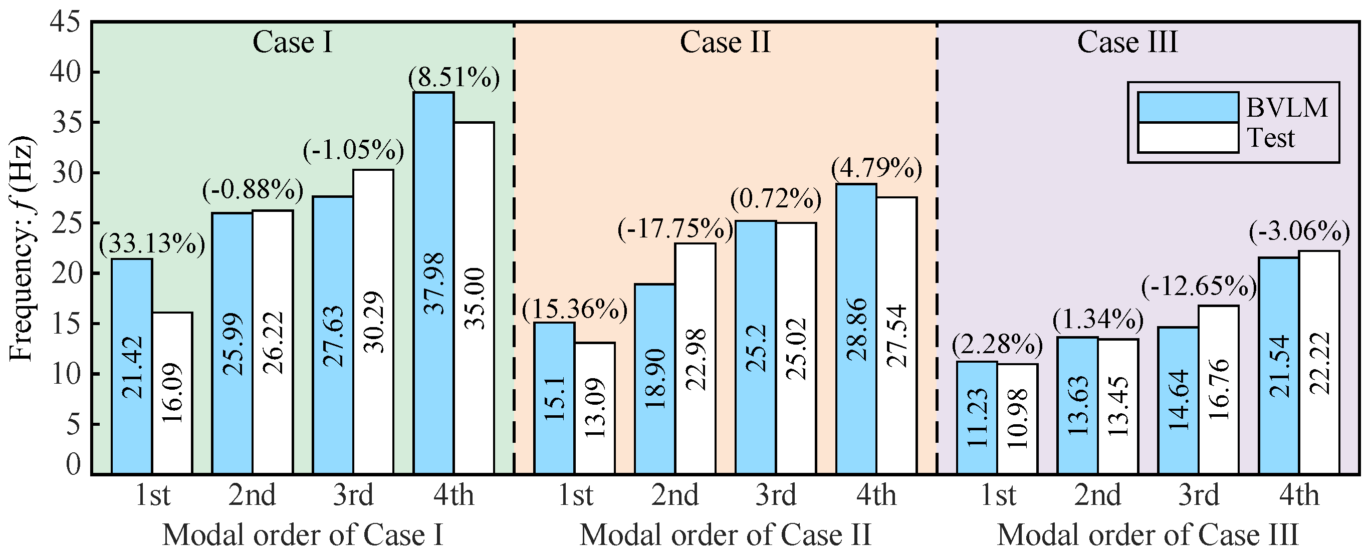
Figure 15 compares the first four natural frequencies predicted by the BVLM-based free-vibration formulation with the corresponding experimental measurements for the three membrane specimens. The associated relative errors, ${\delta }_c$, are reported in brackets above each bar.

Across all 12 modal-frequency comparisons, the mean absolute relative error is $\overline{|{\delta }_c|}=8.46\%$. As a reference, excluding the first mode of Case I reduces this value to 6.22%; however, the all-mode result is retained as the primary indicator of predictive deviation. These results indicate that the free-vibration formulation established from the BVLM-predicted prestress field generally reproduces the modal-frequency evolution with the membrane aspect ratio, while mode-dependent discrepancies remain for several low-order modes. The following discussion examines the predictive accuracy and potential sources of discrepancy for each specimen.

In Case I, the predicted second through fourth natural frequencies agree well with the experimental results, with relative errors of $-0.88\%$, $-1.05\%$, and $8.51\%$, respectively. The largest discrepancy occurs in the first mode: the predicted frequency is $21.42\mathrm{Hz}$, compared with the measured value of $16.09\mathrm{Hz}$, corresponding to a relative error of $33.13\%$. This mode is dominated by global motion of the entire membrane and is therefore particularly sensitive to deviations in the actual boundary conditions and prestress state. Minor changes in the effective membrane tension and global stiffness, induced by slight deformation of the corner-tensioning fixture, microslip at the connections, or local prestress relaxation, can produce a substantial shift in the first natural frequency. In contrast, the second through fourth modes exhibit more localized deformation patterns and are less sensitive to small boundary imperfections and local prestress variations, resulting in markedly smaller prediction errors. These observations suggest that the BVLM-predicted prestress field reproduces the modal response of the principal membrane area, whereas the first global mode remains sensitive to deviations in the actual boundary condition and prestress state.

In Case II, the theoretical and experimental results exhibit consistent overall trends, and all four predicted frequencies remain in ranges comparable to the measured values. The third and fourth modes show particularly close agreement, with relative errors of only $0.72\%$ and $4.79\%$, respectively, indicating that the formulation accurately represents the equivalent stiffness of the membrane in these vibration states. By contrast, the predicted first-mode frequency is slightly higher than the experimental value, whereas the predicted second-mode frequency is lower, with relative errors of $15.36\%$ and $-17.75\%$, respectively. The opposite signs of these deviations indicate that the two lower-order modes respond differently to deviations in the actual tension state, corner connection conditions, and initial membrane geometry. Such deviations can alter the modal stiffness distribution in a mode-dependent manner, causing the first and second natural frequencies to shift in opposite directions relative to the idealized prediction. Taken together, these results show that the proposed model reproduces the principal natural-frequency levels and modal evolution of the Case II membrane with satisfactory accuracy.

In Case III, the theoretical predictions also show good overall agreement with the experimental results. The relative errors of the first, second, and fourth natural frequencies are $2.28\%$, $1.34\%$, and $-3.06\%$, respectively, demonstrating that the model accurately captures the principal vibration characteristics at this aspect ratio, including the low-order global response and the stiffness level associated with the fourth mode. The predicted third-mode frequency is $12.65\%$ lower than the measured value, indicating greater sensitivity of this mode to the actual specimen condition. Variations in local prestress distribution, corner connection conditions, small initial geometric imperfections, and coupling with adjacent modes may increase the effective dynamic stiffness measured in the experiment relative to that predicted by the idealized model. The relatively small errors observed for most modes support the ability of the BVLM model to describe the principal dynamic response of elongated corner-tensioned rectangular membranes.

Across the three specimens, the BVLM-based free-vibration formulation provides reliable predictions of the first four natural frequencies for corner-tensioned rectangular membranes with different aspect ratios and captures the overall reduction in modal frequencies as the membrane length increases. The close agreement between the predicted and measured modal frequencies, particularly for modes with well-defined deformation characteristics, also provides indirect evidence of the dynamic consistency of the BVLM-predicted prestress field. This agreement is consistent with the predicted prestress distribution reproducing both the overall tension level and the spatial stiffness characteristics that govern the membrane dynamic response. The relatively larger discrepancies observed in several lower-order modes are mainly associated with their greater sensitivity to corner constraints, the actual prestress state, and initial geometric imperfections. Collectively, these results support the mechanical consistency of the proposed prestress-field formulation and demonstrate its applicability to rapid free-vibration analysis and modal design of corner-tensioned rectangular membranes.

5. Conclusions

This study develops a Boundary Virtual Load Method (BVLM) for the in-plane prestress prediction of corner-tensioned rectangular membranes. The method addresses residual boundary-normal stresses generated by conventional infinite-domain stress superposition along nominally free edges. An initial prestress field is established from the superposition of radial stress solutions associated with the four corner loads, and the resulting boundary-normal stress residuals are explicitly identified. Boundary virtual loads with equal magnitudes and opposite directions are subsequently introduced to compensate for these residuals and approximate the zero-normal-traction condition along the free boundaries. The virtual load distributions are represented by polynomial functions, from which the corresponding Airy stress functions are derived to obtain a polynomially corrected, closed-form representation of the prestress field.

The proposed method is assessed using three membrane cases with different aspect ratios. Comparisons with finite element results indicate that BVLM captures the principal features of the in-plane stress distributions, including the corner stress concentrations, edge-dominated stress characteristics, and aspect-ratio-dependent evolution of the stress field. In addition, BVLM predicts the stress field at lower computational cost than the finite element method for the cases and computational settings examined. These results support the applicability of the boundary-corrected representation for efficient prestress evaluation in the examined membrane configurations.

The predicted prestress fields are further incorporated into a free-vibration formulation that accounts for the added-mass effect of the surrounding air. The predicted first four natural frequencies generally reproduce the measured modal-frequency trends, although mode-dependent discrepancies remain, particularly for several low-order modes. The mean absolute relative error of the 12 modal-frequency comparisons is $8.46\%$, which decreases to $6.22\%$ after excluding the largest deviation associated with the first mode of Case I. The model also captures the overall reduction in modal frequencies as the membrane aspect ratio increases. The overall correspondence between the predicted and measured modal characteristics therefore provides an indirect dynamic consistency assessment of the BVLM-based prestressed vibration model, while the observed mode-dependent discrepancies indicate that the modal predictions should be interpreted as approximate rather than uniformly high-accuracy predictions.

Overall, BVLM provides a semi-analytical and computationally efficient framework for prestress-field prediction and preliminary free-vibration analysis of homogeneous rectangular membranes subjected to equal diagonal corner tensions within a prescribed fixed geometry and globally taut state. Within this validated domain, the method provides a practical tool for rapid stress evaluation, modal characterization, and parametric design. Future work will focus on extending the BVLM framework to nonrectangular membrane geometries. This extension will involve constructing geometry-dependent initial stress fields, redefining the residual traction distributions along irregular boundaries, and developing corresponding boundary virtual-load functions and Airy stress-function solutions for more general membrane shapes.

References

1. Feng, C.; Liu, T. A bionic approach to mathematical modeling the fold geometry of deployable reflector antennas on satellites. Acta Astronaut. 2014, 103, 36–44. [Google Scholar] [CrossRef] [Scilit]
2. Chen, J.; Shi, A.; He, Y.; Dai, H.; Pei, Y. Nonlinear nonmodal analysis of solar sail orbit robust stability. Acta Astronaut. 2025, 236, 755–769. [Google Scholar] [CrossRef] [Scilit]
3. Senda, K.; Petrovic, M.; Nakanishi, K. Wrinkle generation in shear-enforced rectangular membrane. Acta Astronaut. 2015, 111, 110–135. [Google Scholar] [CrossRef] [Scilit][Green Version]
4. Pimprikar, N.; Banerjee, B.; Roy, D.; Vasu, R.; Reid, S. New computational approaches for wrinkled and slack membranes. Int. J. Solids Struct. 2010, 47, 2476–2486. [Google Scholar] [CrossRef] [Scilit]
5. Sheng, L.; Zhang, Y.; Xu, J.; Li, X.; Zhao, Y. Tearing behavior of PVC-coated fabric with double initial cracks. Thin-Walled Struct. 2025, 211, 113103. [Google Scholar] [CrossRef] [Scilit]
6. Orszulik, R.R.; Shan, J. Fuzzy logic active flatness control of a space membrane structure. Acta Astronaut. 2012, 77, 68–76. [Google Scholar] [CrossRef] [Scilit]
7. Aoki, T.; Ishimura, K. New concept of compressive load transmitting member applicable to large space structures. Acta Astronaut. 2010, 67, 449–454. [Google Scholar] [CrossRef] [Scilit]
8. Xu, X.; Yan, H.; Wang, G.; Yao, X. Full-size mechanical evaluation for large aircraft cabin door with complex fabric rubber composite seal structures. Aerosp. Sci. Technol. 2025, 166, 110581. [Google Scholar] [CrossRef] [Scilit]
9. Song, S.; Jin, H. Identifying constitutive parameters for complex hyperelastic materials using physics-informed neural networks. Soft Matter 2024, 20, 5915–5926. [Google Scholar] [CrossRef] [Scilit]
10. Kang, Y.; Li, Y.; Li, W.; Li, H.; Liu, T.; Lu, F.; Ma, B.; Tian, X.; Li, D. Multi-level approximating 3D printing of curved surface with continuous carbon fiber for solid parabolic antenna. J. Manuf. Process. 2026, 158, 363–373. [Google Scholar] [CrossRef] [Scilit]
11. Pipkin, A.C. Lectures on Viscoelasticity Theory; Springer Science & Business Media: Berlin/Heidelberg, Germany, 2012; Volume 7. [Google Scholar]
12. Wang, T.; Yang, Y.; Xu, F. Mechanics of tension-induced film wrinkling and restabilization: A review. Proc. R. Soc. A 2022, 478, 20220149. [Google Scholar] [CrossRef] [Scilit]
13. Nayyar, V.; Ravi-Chandar, K.; Huang, R. Stretch-induced stress patterns and wrinkles in hyperelastic thin sheets. Int. J. Solids Struct. 2011, 48, 3471–3483. [Google Scholar] [CrossRef] [Scilit]
14. Libai, A. The Nonlinear Theory of Elastic Shells: One Spatial Dimension; Elsevier: Amsterdam, The Netherlands, 2012. [Google Scholar]
15. Li, Q.; Healey, T.J. Stability boundaries for wrinkling in highly stretched elastic sheets. J. Mech. Phys. Solids 2016, 97, 260–274. [Google Scholar] [CrossRef] [Scilit]
16. Janssens, S.D.; Sutisna, B.; Giussani, A.; Kwiecinski, J.A.; Vázquez-Cortés, D.; Fried, E. Boundary curvature effect on the wrinkling of thin suspended films. Appl. Phys. Lett. 2020, 116, 193702. [Google Scholar] [CrossRef] [Scilit]
17. Zhang, D.; Kiendl, J. A variationally consistent membrane wrinkling model based on spectral decomposition of the strain tensor. Comput. Methods Appl. Mech. Eng. 2024, 432, 117386. [Google Scholar] [CrossRef] [Scilit]
18. Xu, J.; Sheng, L.; Zhang, Y.; Fei, S.; Zhao, Z. A novel end-to-end deep learning model for predicting the full stress field of tensioned membrane structures. KSCE J. Civ. Eng. 2025, 29, 100073. [Google Scholar] [CrossRef] [Scilit]
19. Iwasa, T.; Fujibayashi, S.; Katsumata, N.; Higuchi, K. Upper-bound vibration response spectrum computation for deployable membrane structures with uncertainty effects. Thin-Walled Struct. 2024, 198, 111706. [Google Scholar] [CrossRef] [Scilit]
20. Song, P.; Cai, L.; Li, W.; Cao, X.; Jin, Y.; Elbugdady, I. Non-uniform stress distribution characteristics and structure-related modeling approach of proton exchange membrane under durability protocol conditions. Int. J. Green Energy 2025, 22, 2046–2064. [Google Scholar] [CrossRef] [Scilit]
21. Van Phan, H.; Coşkun, M.B.; Şeşen, M.; Pandraud, G.; Neild, A.; Alan, T. Vibrating membrane with discontinuities for rapid and efficient microfluidic mixing. Lab Chip 2015, 15, 4206–4216. [Google Scholar] [CrossRef] [Scilit]
22. Bereyhi, M.J.; Beccari, A.; Groth, R.; Fedorov, S.A.; Arabmoheghi, A.; Kippenberg, T.J.; Engelsen, N.J. Hierarchical tensile structures with ultralow mechanical dissipation. Nat. Commun. 2022, 13, 3097. [Google Scholar] [CrossRef] [Scilit]
23. Melnyk, V. Soft Knitted Tensile Membrane Tensegrity Helix-Tower. Enq. ARCC J. Archit. Res. 2023, 20, 60–68. [Google Scholar] [CrossRef] [Scilit]
24. Galhofo, D.; Silvestre, N.; de Deus, A.M.; Reis, L.; Duarte, A.P.; Carvalho, R. Structural behaviour of pre-tensioned solar sails. Thin-Walled Struct. 2022, 181, 110007. [Google Scholar] [CrossRef] [Scilit]
25. Gorman, D.; Singhal, R.; Graham, W.; Crawford, J. Investigation of the stress distributions in corner tensioned rectangular membranes. AIAA J. 1993, 31, 2361–2366. [Google Scholar] [CrossRef] [Scilit]
26. Liu, M.; Huang, J.; Wang, Y. Analysis of wrinkled membrane structures based on a wrinkle-wave model. AIP Adv. 2017, 7, 015301. [Google Scholar] [CrossRef] [Scilit]
27. Wong, Y.; Pellegrino, S.; Park, K. Prediction of winkle amplitudes in square solar sails. In Proceedings of the 44th AIAA/ASME/ASCE/AHS/ASC Structures, Structural Dynamics, and Materials Conference, Norfolk, VA, USA, 7–10 April 2003; p. 1982. [Google Scholar]
28. Li, B.; Liu, R.; Cong, Q.; Guo, H.; Lin, Q. Stress Superposition Method and free vibration of corner tensioned rectangular thin membranes. Thin-Walled Struct. 2021, 159, 107201. [Google Scholar] [CrossRef] [Scilit]
29. Sun, P.; Huang, J.; Zhang, J.; Meng, F. Wrinkling patterns and stress analysis of tensile membrane with rigid elements. Appl. Sci. 2022, 12, 6630. [Google Scholar] [CrossRef] [Scilit]
30. Tang, Y.; Guo, H.; Liu, R.; Deng, Z. Space membrane wrinkle analytical model based on piecewise stress field. Thin-Walled Struct. 2023, 189, 110869. [Google Scholar] [CrossRef] [Scilit]
31. Chao, C.C. Elastodynamics, Vol. II, Linear Theory. J. Appl. Mech. 1978, 45, 229. [Google Scholar] [CrossRef] [Scilit][Green Version]
32. Goodier, J.N.; Timoshenko, S. Theory of Elasticity; McGraw-Hill: New York, NY, USA, 1970; Volume 2. [Google Scholar]
33. Liu, X.; Cai, G.; Peng, F.; Zhang, H. Piezoelectric actuator placement optimization and active vibration control of a membrane structure. Acta Mech. Solida Sin. 2018, 31, 66–79. [Google Scholar] [CrossRef] [Scilit]
34. Minami, H. Added mass of a membrane vibrating at finite amplitude. J. Fluids Struct. 1998, 12, 919–932. [Google Scholar] [CrossRef] [Scilit]
Figure 1. Geometric and prestress-field description of a corner-tensioned rectangular membrane. (a) Schematic of a large-aperture membrane structure maintained by corner-applied tensile forces. (b) Rectangular membrane model with dimensions 2 a × 2 b , where four identical tensile forces T are applied at the corner points A i   ( i = 1 ,   2 ,   3 ,   4 ) along the diagonal directions. (c) Coordinate transformation for evaluating the stress components at point C ( x , y ) .
Machines 14 00971 g001
Figure 2. Boundary stress components and residual stresses of the initial prestress field. (a) Decomposition of the corner tension into the x- and y-directional components, indicating that only the tangential normal-stress component is physically applied along the membrane boundary. (b) Residual boundary-normal stress σ y 1 and shear stress τ x y 1 along y = b . (c) Residual boundary-normal stress σ x 1 and shear stress τ x y 1 along x = a . Results are shown for a 400 mm × 200 mm × 0.025 mm membrane subjected to a corner tension of 1 N .
Machines 14 00971 g002
Figure 3. Distribution characteristics and evolution trends of the boundary-normal stress residuals σ n x 1 and σ n y 1 under different geometric conditions. (a–d) Results obtained with b = 200 mm as a increases from 200 mm to 800 mm : (a) σ n y 1 along the top edge; (b) σ n y 1 at the midpoint and endpoints of the top edge; (c) σ n x 1 along the right edge; and (d) σ n x 1 at the midpoint and endpoints of the right edge. (e–h) Results obtained with a = 2 b as a increases from 200 mm to 800 mm : (e) σ n y 1 along the top edge; (f) σ n y 1 at the midpoint and endpoints of the top edge; (g) σ n x 1 along the right edge; and (h) σ n x 1 at the midpoint and endpoints of the right edge.
Machines 14 00971 g003
Figure 4. Schematic illustration of the boundary virtual-load correction. The equivalent virtual loads F n x and F n y are applied along the membrane edges to compensate for the boundary-normal stress residuals σ n x 1 and σ n y 1 generated by the initial prestress field, thereby approximating the zero-normal-traction boundary condition.
Machines 14 00971 g004
Figure 5. Polynomial-degree selection, sixth-order fitting, and residual evaluation of the boundary virtual loads. Panels (a–c) compare the training root-mean-square error (TR RMSE) and five-fold cross-validated root-mean-square error (CV RMSE, mean ± standard deviation) for candidate polynomial degrees of (a) F n y at k = 1 , (b) F n y at k = 6 , and (c) F n x at k = 6 . Panels (d–f) compare the sixth-order polynomial fits with the discrete virtual-load data for (d) F n y at k = 1 , (e) F n y at k = 6 , and (f) F n x at k = 6 , while panels (g–i) present the corresponding fitting residuals. Only every fifth discrete data point is displayed in the fitting plots for clarity.
Machines 14 00971 g005
Figure 6. Geometric configurations and boundary loading conditions of the three membrane case studies: (a) Case I; (b) Case II; and (c) Case III. A diagonal tensile load of 10 N is applied at each corner.
Machines 14 00971 g006
Figure 7. BVLM-predicted in-plane prestress distributions (unit: MPa) of the three membrane case studies under corner diagonal tensile loading: (a) normal stress σ x for Case I; (b) normal stress σ x for Case II; (c) normal stress σ x for Case III; (d) normal stress σ y for Case I; (e) normal stress σ y for Case II; (f) normal stress σ y for Case III; (g) shear stress τ x y for Case I; (h) shear stress τ x y for Case II; and (i) shear stress τ x y for Case III.
Machines 14 00971 g007
Figure 8. Mesh-independence verification for the finite element stress analysis: (a) structured square-element discretization and stress-monitoring point p ( 0.8 a , 0.8 b ) ; (b) mesh-convergence curves of the stress components for Case I; (c) mesh-convergence curves of the stress components for Case II; and (d) mesh-convergence curves of the stress components for Case III.
Machines 14 00971 g008
Figure 9. Finite-element-predicted in-plane prestress distributions (unit: MPa) of the three membrane case studies under corner diagonal tensile loading: (a) normal stress σ x for Case I; (b) normal stress σ x for Case II; (c) normal stress σ x for Case III; (d) normal stress σ y for Case I; (e) normal stress σ y for Case II; (f) normal stress σ y for Case III; (g) shear stress τ x y for Case I; (h) shear stress τ x y for Case II; and (i) shear stress τ x y for Case III.
Machines 14 00971 g009
Figure 10. Locations of the four representative cross-sections ( S 1 – S 4 ) used for extracting and comparing stress profiles between the BVLM predictions and finite element results.
Machines 14 00971 g010
Figure 11. Comparative analysis of stress profiles predicted by the BVLM and FEM along representative cross-sections ( S 1 – S 4 ) for the three cases: (a) normal stress σ x for Case I; (b) normal stress σ x for Case II; (c) normal stress σ x for Case III; (d) normal stress σ y for Case I; (e) normal stress σ y for Case II; (f) normal stress σ y for Case III; (g) shear stress τ x y for Case I; (h) shear stress τ x y for Case II; and (i) shear stress τ x y for Case III.
Machines 14 00971 g011
Figure 12. Computation times for (a) BVLM and (b) FEM.
Machines 14 00971 g012
Figure 13. Modal experiment setup. (a) Three experimental specimens corresponding to analysis Cases I–III; (b) experimental test setup.
Machines 14 00971 g013
Figure 14. Experimental frequency response functions of the prestressed membrane specimens: (a) Case I; (b) Case II; and (c) Case III.
Machines 14 00971 g014
Figure 15. Comparison of BVLM-predicted and experimentally measured natural frequencies. Bar chart of the first four natural frequencies for the three cases; values in parentheses above the bars denote the relative error δ c .
Machines 14 00971 g015