A Comprehensive Review of Modeling and Control Techniques of LCC-HVDC and VSC-HVDC Systems

Abstract

The rapid advancement of power electronic devices has accelerated the widespread adoption of Line-Commutated Converter (LCC) and Voltage Source Converter (VSC) technologies as leading solutions for high-voltage industrial applications. These technologies have become fundamental components of modern high-voltage direct current (HVDC) transmission systems and advanced Industrial Machine-Drive (IMD) systems. This review presents a comprehensive comparison between conventional LCC technology and the more recent VSC technology, highlighting the operational advantages, limitations, and application suitability of each approach. In addition, it provides an in-depth examination of hierarchical control architectures employed in both LCC-HVDC and VSC-HVDC systems. As these systems are increasingly required to operate closer to their performance limits, the implementation of robust and efficient control strategies has become essential for ensuring stability, reliability, and optimal performance. Consequently, a wide range of control techniques has been developed to address the inherent nonlinearities and parameter uncertainties present in power systems. This review evaluates and compares both conventional and advanced control methods, including Proportional–Integral (PI) control, Variable Coefficient PI (V-PI), Fuzzy PI, Self-Tuning Fuzzy PI (STF-PI), Fractional Order PI (FOPI), Variable Coefficient Fractional Order PI (V-FOPI), Adaptive Neuro-Fuzzy Inference Systems (ANFIS), and Model Predictive Control (MPC). Their performance is assessed across a range of operating conditions, with emphasis on dynamic response, robustness, and overall control effectiveness.

1. Introduction

1.1. Background

Line-Commutated Converter (LCC) and Voltage Source Converter (VSC) technologies have emerged as the dominant solutions for industrial high-voltage applications. The integration of these two distinct topologies has driven a radical transformation in two critical energy-intensive sectors. On the power grid level, these converters form the backbone of modern high-voltage direct current (HVDC) transmission systems, which are essential for integrating renewable energy and interconnecting asynchronous grids. Beyond HVDC transmission, LCC and VSC are equally vital within advanced machine-drive systems; these converters deliver the precise and reliable control of high-power machines required by heavy industries such as mining, oil and gas, and marine propulsion.

The increasing demand for electricity requires continuous development plans to enhance generating capacity, transmission capabilities, and facilitate the linkage of areas separated by vast distances. The requirement for transferring electrical power across the ocean is fairly common, in addition to the need to connect asynchronous systems with various frequencies, where traditional alternating current AC connections cannot be used. This requires identifying technical and cost-effective technologies that guarantee stability and manage appropriate energy exchange. The only efficient option is to utilize high-voltage direct current (HVDC) transmission systems. HVDC transmission is a major technology used in modern power systems, permitting effective bulk power transfer over vast distances, interconnecting asynchronous AC grids, integrating large-scale renewable energy sources, and enhancing overall system stability and controllability [1,2].

HVDC systems are categorized into two types: Line-Commutated Converters (LCC-HVDC) and Voltage Source Converters (VSC-HVDC), each with its own modeling and control mechanisms. Traditionally, HVDC systems employ Line-Commutated Converters (LCCs) based on thyristor valves. These electronic valves employ the AC grid voltage for commutation. They are ideal for high-power, long-distance connections with robust AC systems. The drawbacks of this transmission technique include reactive power absorption, harmonics, difficulty in multi-terminal and weak-grid applications, commutation failure, and the inability to turn off valves or thyristors directly with gate signals. These drawbacks limit the scope of its application. In contrast, the emergence of Voltage Source Converters (VSCs) employing Insulated Gate Bipolar Transistors (IGBTs) established a novel generation of HVDC systems. These systems offer fast, flexible, and bidirectional control over active as well as reactive power, are capable of connecting to weak or passive AC grids, and have improved power-quality characteristics [3].

The primary distinction that exists between the standard LCC and the recently introduced VSC is that the new VSC utilizes elements that are capable of turning off the current rather than just turning it on. These turn-off elements are IGBTs. Because the current in a VSC can be turned off, there is no requirement for commutation voltage in the connected AC networks. Therefore, by using this kind of converter, the AC current is capable of leading or lagging the AC voltage, which means that the converter is able to absorb or provide reactive power to the linked AC networks [3].

The increasing complexity and diversity of HVDC applications create significant modeling and control design challenges. On the modeling part, precise dynamic models of converter switching behavior, AC-DC coupling, and control loops are critical for stability analysis, optimal control, and real-time simulations. On the control side, the goal is to design robust and high-performance control techniques in HVDC transmission systems that are capable of: controlling active and reactive power flows, ensuring DC voltage stability, maintaining system synchronization with weak AC networks, protecting from faults and disturbances, ensuring grid stability and frequency regulation, maintaining power flow during dynamic events, and improving system efficiency. Without proper control, HVDC systems will suffer from instability, component damage, and an inability to support the connected AC networks effectively [4].

1.2. Review Methodology

To construct a comprehensive and unbiased overview of HVDC modeling and control, a structured literature search was conducted across primary scientific databases, including IEEE Xplore, Scopus, and Web of Science. The search queries combined terminology related to converter topologies (e.g., “LCC-HVDC,” “VSC-HVDC,” “MMC-HVDC”) with terms denoting analytical and control methodologies (e.g., “dynamic modeling,” “hierarchical control,” “fuzzy logic,” “predictive control”). While the primary focus of the broader review spans the last fifteen years to capture recent technological leaps and foundational developments, a dedicated emphasis has been placed on the absolute frontier of the field. As such, the detailed comparative analysis presented in Table 5 exclusively features, categorizes, and evaluates very recent research publications from the year 2025, ensuring the manuscript captures the absolute latest state-of-the-art advancements. This table synthesizes findings from both the latest primary research articles proposing novel controller designs and contemporary review papers that offer updated taxonomies, benchmarking, and critical perspectives on these advanced control techniques applied to both modern high-voltage direct current (HVDC) transmission systems and advanced Industrial Machine-Drive (IMD) systems.

To maintain a strict focus on HVDC control design and system-level modeling, we excluded studies that lacked proper validation, focused purely on device physics, or proposed hardware without control analysis. Specifically, the literature has been classified according to the following criteria:

•

Converter Technology: Distinguishing between classical Line-Commutated Converters (LCC), standard two-level Voltage Source Converters (VSC), and modern modular multilevel converters (MMC), as the inherent hardware differences dictate entirely different control requirements.

•

Modeling Approach: Steady-state, averaged, dynamic, detailed switching, and reduced-order models.

•

Control Architecture: Mapping the literature to standard hierarchical layers of HVDC control, specifically differentiating between supervisory system-level coordination, outer power and voltage loops, and high-bandwidth inner current-regulation loops.

•

Controller Type: Grouping the actual control algorithms implemented within the aforementioned loops. This spans from conventional Proportional–Integral (PI) regulators to advanced topologies like Variable Coefficient PI (V-PI), Fuzzy PI, Fractional Order PI (FOPI), Adaptive Neuro-Fuzzy Inference Systems (ANFIS), and Model Predictive Control (MPC).

•

Optimization and Adaptation Method: Meta-heuristic optimization utilized specifically for offline or online parameter tuning of the aforementioned controllers.

•

Application Domain: VSC-HVDC integration within high-voltage direct current transmission systems and high-power Industrial Machine Drive.

•

Operating Condition and Validation Method: Categorizing papers based on the specific grid strengths tested (strong versus weak AC networks), the disturbance scenarios analyzed, and the simulation or hardware platforms used to validate the claims.

1.3. Rationale for Comparing HVDC Transmission and Machine-Drive Control Strategies

Despite the fact that high-voltage direct current (HVDC) transmission and high-power electric machine drives serve fundamentally different industrial purposes. The comparison between HVDC systems and electric machine drives is motivated by the strong methodological and mathematical similarities in their converter-level control structures.

In particular, the fundamental inner control loops, including dq-frame current regulation, decoupling of cross-coupled current components, and voltage/current control, are based on closely related mathematical formulations in high-power VSC-HVDC systems and medium-voltage variable-frequency machine drives. Both applications also present common advanced control challenges associated with nonlinear system behavior, parameter uncertainty, cross-coupling, disturbances, and the requirement for fast dynamic tracking [5].

Machine-drive research has also developed and validated a wide range of advanced control and optimization techniques, including Model Predictive Control (MPC), Adaptive Neuro-Fuzzy Inference Systems (ANFIS), fuzzy-based control, fractional order control, and optimization-based parameter tuning. The experience gained from these applications provides relevant methodological insight for HVDC controller development, particularly at the converter-control level. However, we acknowledge that the two application domains have different system-level objectives and constraints. HVDC control primarily addresses requirements such as DC voltage regulation, active/reactive power control, AC grid interaction, and power flow regulation, whereas machine-drive control focuses on variables such as torque, speed, flux, and machine current. Therefore, this review does not treat machine-drive results as directly equivalent to HVDC performance results. Instead, machine-drive studies are used to demonstrate the development and applicability of advanced converter-control methodologies that may be relevant to HVDC applications [6,7].

1.4. Scope, Evaluation Criteria, and Principal Contributions

As the field of HVDC transmission becomes more advanced, the literature has become saturated with diverse control topologies and tuning methods. The principal contribution of this review is not the proposal of a new controller, but rather the systematic synthesis, classification, and critical comparative evaluation of existing methodologies to provide clear engineering guidance. To achieve this, the review is structured around the following key contributions:

•

Systematic comparison of the transition from LCC-HVDC to VSC-HVDC: The review examines the evolution from conventional LCC-HVDC to VSC-HVDC, highlighting the associated changes in converter characteristics, modeling requirements, control capabilities, limitations, and application suitability.

•

Hierarchical classification of control strategies: The reviewed controllers are systematically categorized according to the hierarchical control level and control function they address, rather than being considered as an undifferentiated collection of control techniques. This provides a clearer relationship between converter control objectives, control architecture, and controller selection.

•

Identification of trends in advanced control: The synthesis of the reviewed studies indicates that conventional controllers, particularly fixed-parameter PI control, remain attractive because of their simplicity and low computational requirements, but may face limitations under nonlinearities, parameter variations, and significant disturbances. The literature further indicates that advanced approaches, including fuzzy logic, neuro-fuzzy methods, fractional order control, predictive control, and optimization-assisted tuning, can provide improved dynamic performance and robustness in appropriate operating conditions, although these benefits are generally accompanied by increased computational and implementation complexity. Thus, the review identifies a clear performance–complexity trade-off, rather than claiming that one controller is universally superior.

•

Integrated analysis of VSC control strategies across relevant applications: The review provides a structured analysis of VSC control strategies reported for HVDC systems and, where relevant, high-performance machine-drive applications. The latter are included to identify transferable converter-level control methodologies, while recognizing that the two application domains have different system-level objectives and constraints.

•

Comparative qualitative evaluation of the reviewed literature: Rather than simply listing previously published controllers, the manuscript synthesizes the evidence reported in the selected studies and provides a comparative assessment in Table 5. The assessment considers the methodology employed, the performance claims made by the authors, the reported performance metrics, and a critical review of the advantages in addition to the limitations of the respective approaches. Table 6 offers a qualitative, side-by-side comparison of seven widely studied controllers commonly reported in HVDC and machine-drive control literature, ranging from conventional PI to Model Predictive Control, and rates each on dynamic response, robustness, complexity, real-time suitability, and overall performance.

In addition, Section 13 discusses the principal advantages and disadvantages of each controller and explains the circumstances in which each approach may be appropriate for VSC-HVDC applications. Importantly, because the reviewed studies employ different converter topologies, system ratings, operating conditions, performance indices, and simulation or experimental platforms, the qualitative assessment is not intended to constitute a universal numerical ranking. Instead, it represents a literature-based synthesis of the reported evidence. The manuscript therefore makes a clearer distinction between what has previously been reported in the literature and the new synthesis generated by this review. The principal result of the review is the identification of the relationships and trade-offs between converter topology, hierarchical control level, controller sophistication, dynamic performance, robustness, and implementation complexity, which provides guidance for selecting appropriate control strategies for different VSC-HVDC operating requirements.

2. Mathematical Modeling of HVDC Systems

This section presents the mathematical and control-oriented models for the three principal HVDC converter technologies: Line-Commutated Converters (LCC), two-level Voltage Source Converters (VSC), and modular multilevel converters (MMC). Each subsection develops the governing equations, reference-frame transformations, and hierarchical control structure. These models provide the foundation for time-domain simulation of LCC-, VSC-, and MMC-based HVDC links, enabling comparative studies of dynamic performance, fault response, and control interaction in hybrid AC/DC grids [8].

2.1. LCC-HVDC Modeling

Line-Commutated Converters rely on external AC line voltages for thyristor commutation. The classical 12-pulse converter configuration consists of two 6-pulse bridge rectifiers connected in series, powered by star-star (Y-Y) and star-delta (Y-Δ) converter transformers to eliminate the 5th and 7th harmonic orders [8,9].

(a)

DC Output Voltage Equations

The average DC voltage generated by a 6-pulse bridge under ideal conditions is expressed as a function of the firing angle $\mathsf{\alpha }$:

$${\mathrm{V}}_{\mathrm{d}\mathrm{c}0}={\displaystyle \frac{3\sqrt{2}}{\mathsf{\pi }}}{\mathrm{V}}_{\mathrm{L}\mathrm{L}}\cos \mathsf{\alpha }$$

(1)

where ${\mathrm{V}}_{\mathrm{L}\mathrm{L}}$ represents a line-to-line RMS voltage at a converter transformer secondary.

Accounting for the commutation overlap angle ($\mathsf{\mu }$) caused by transformer leakage reactance (${\mathrm{X}}_{\mathrm{c}}$), the continuous average DC voltage equation for an LCC rectifier is defined as:

$${\mathrm{V}}_{\mathrm{d}\mathrm{c},\mathrm{R}}={\displaystyle \frac{3\sqrt{2}}{\mathsf{\pi }}}{\mathrm{V}}_{\mathrm{L}\mathrm{L}}\cos \mathsf{\alpha }-{\displaystyle \frac{3}{\mathsf{\pi }}}{\mathrm{X}}_{\mathrm{c}}{\mathrm{I}}_{\mathrm{d}\mathrm{c}}$$

(2)

For inverter operation, where the converter operates with an extinction angle ($\mathsf{\gamma }=\mathsf{\pi }-\mathsf{\alpha }-\mathsf{\mu }$), the DC voltage formulation becomes:

$${\mathrm{V}}_{\mathrm{d}\mathrm{c},\mathrm{I}}={\displaystyle \frac{3\sqrt{2}}{\mathsf{\pi }}}{\mathrm{V}}_{\mathrm{L}\mathrm{L}}\cos \mathsf{\gamma }-{\displaystyle \frac{3}{\mathsf{\pi }}}{\mathrm{X}}_{\mathrm{c}}{\mathrm{I}}_{\mathrm{d}\mathrm{c}}$$

(3)

(b)

Dynamic Line Model and Current Control

The equivalent DC link connecting the rectifier ($\mathrm{R}$) and inverter ($\mathrm{I}$) stations is modeled as an R-L series circuit:

$${\mathrm{L}}_{\mathrm{d}\mathrm{c}}{\displaystyle \frac{\mathrm{d}{\mathrm{I}}_{\mathrm{d}\mathrm{c}}}{\mathrm{d}\mathrm{t}}}+{\mathrm{R}}_{\mathrm{d}\mathrm{c}}{\mathrm{I}}_{\mathrm{d}\mathrm{c}}={\mathrm{V}}_{\mathrm{d}\mathrm{c},\mathrm{R}}-{\mathrm{V}}_{\mathrm{d}\mathrm{c},\mathrm{I}}$$

(4)

where ${\mathrm{L}}_{\mathrm{d}\mathrm{c}}$ and ${\mathrm{R}}_{\mathrm{d}\mathrm{c}}$ denote the total smoothing reactor inductance and line resistance, respectively. This equation governs the DC current dynamics and is used to close the loop between rectifier and inverter models.

(c)

Hierarchical Control Structure

LCC control relies on a single degree of freedom: the thyristor firing angle. The standard hierarchical control comprises:

•

Current Control (Rectifier): A PI regulator adjusts the firing angle $\mathsf{\alpha }$ to track a reference DC current ${\mathrm{I}}_{\mathrm{d}\mathrm{c}}^{\ast }$, using the error $\mathrm{e}={\mathrm{I}}_{\mathrm{d}\mathrm{c}}^{\ast }-{\mathrm{I}}_{\mathrm{d}\mathrm{c}}$.

•

Voltage/Extinction Angle Control (Inverter): A second PI loop regulates the extinction angle $\mathsf{\gamma }$ to maintain a minimum extinction angle for safe commutation and to support DC voltage.

•

Current Margin Method: The inverter current reference is set slightly below the rectifier reference (${\mathrm{I}}_{\mathrm{d}\mathrm{c},\mathrm{I}}^{\ast }={\mathrm{I}}_{\mathrm{d}\mathrm{c},\mathrm{R}}^{\ast }-{\mathrm{I}}_{\mathrm{m}\mathrm{a}\mathrm{r}\mathrm{g}\mathrm{i}\mathrm{n}}$) to ensure stable current control handover between stations.

2.2. VSC-HVDC Modeling

Unlike LCC systems, VSCs utilize self-commutated Insulated Gate Bipolar Transistors (IGBTs) with Pulse Width Modulation (PWM), permitting independent control of active ($\mathrm{P}$) and reactive ($\mathrm{Q}$) power without requiring an external AC voltage source [10,11].

(a)

AC-side dynamic model in dq frame

The two-level VSC is modeled in the synchronous rotating $\mathrm{d}\mathrm{q}$ reference frame synchronized with the AC grid voltage vector via a Phase-Locked Loop (PLL); the AC dynamic equations in the rotating $\mathrm{d}\mathrm{q}$ frame are described by:

$${\mathrm{L}}_{\mathrm{s}}{\displaystyle \frac{\mathrm{d}{\mathrm{i}}_{\mathrm{d}}}{\mathrm{d}\mathrm{t}}}=-{\mathrm{R}}_{\mathrm{s}}{\mathrm{i}}_{\mathrm{d}}+\mathsf{\omega }{\mathrm{L}}_{\mathrm{s}}{\mathrm{i}}_{\mathrm{q}}+{\mathrm{v}}_{\mathrm{s},\mathrm{d}}-{\mathrm{v}}_{\mathrm{d}}$$

(5)

$${\mathrm{L}}_{\mathrm{s}}{\displaystyle \frac{\mathrm{d}{\mathrm{i}}_{\mathrm{q}}}{\mathrm{d}\mathrm{t}}}=-{\mathrm{R}}_{\mathrm{s}}{\mathrm{i}}_{\mathrm{q}}-\mathsf{\omega }{\mathrm{L}}_{\mathrm{s}}{\mathrm{i}}_{\mathrm{d}}+{\mathrm{v}}_{\mathrm{s},\mathrm{q}}-{\mathrm{v}}_{\mathrm{q}}$$

(6)

where ${\mathrm{i}}_{\mathrm{d}},{\mathrm{i}}_{\mathrm{q}}$ are the converter currents, ${\mathrm{v}}_{\mathrm{d}},{\mathrm{v}}_{\mathrm{q}}$ are the converter terminal voltages (modulation outputs), ${\mathrm{v}}_{\mathrm{s},\mathrm{d}},{\mathrm{v}}_{\mathrm{s},\mathrm{q}}$ are the grid voltages, ${\mathrm{R}}_{\mathrm{s}}$ and ${\mathrm{L}}_{\mathrm{s}}$ represent the equivalent phase resistance and inductance of the interface transformer and phase reactor, and $\mathsf{\omega }$ is the grid angular frequency.

(b)

Decoupled Power Control Formulation

With the PLL locked to the $\mathrm{d}$-axis (${\mathrm{v}}_{\mathrm{s}}={\mathrm{v}}_{\mathrm{d}}$ and ${\mathrm{v}}_{\mathrm{q}}=0$), instantaneous active and reactive power injected into the AC grid simplify to:

$$\mathrm{P}={\displaystyle \frac{3}{2}}{\mathrm{v}}_{\mathrm{d}}{\mathrm{i}}_{\mathrm{d}} , \mathrm{Q}=-{\displaystyle \frac{3}{2}}{\mathrm{v}}_{\mathrm{d}}{\mathrm{i}}_{\mathrm{q}}$$

(7)

Consequently, active power $\mathrm{P}$ (or DC link voltage ${\mathrm{V}}_{\mathrm{d}\mathrm{c}}$) is controlled via the $\mathrm{d}$-axis current reference ${\mathrm{i}}_{\mathrm{d}}^{\ast }$, while reactive power $\mathrm{Q}$ (or AC voltage magnitude ${\mathrm{V}}_{\mathrm{a}\mathrm{c}}$) is independently governed by the $\mathrm{q}$-axis current reference ${\mathrm{i}}_{\mathrm{q}}^{\ast }$:

$${\mathrm{i}}_{\mathrm{d}}^{\ast }={\mathrm{K}}_{\mathrm{p},\mathrm{p}}\left({\mathrm{P}}_{\mathrm{r}\mathrm{e}\mathrm{f}}-\mathrm{P}\right)+{\mathrm{K}}_{\mathrm{i},\mathrm{p}}\int \left({\mathrm{P}}_{\mathrm{r}\mathrm{e}\mathrm{f}}-\mathrm{P}\right)\mathrm{d}\mathrm{t}$$

(8)

$${\mathrm{i}}_{\mathrm{q}}^{\ast }={\mathrm{K}}_{\mathrm{p},\mathrm{q}}\left({\mathrm{Q}}_{\mathrm{r}\mathrm{e}\mathrm{f}}-\mathrm{Q}\right)+{\mathrm{K}}_{\mathrm{i},\mathrm{q}}\int \left({\mathrm{Q}}_{\mathrm{r}\mathrm{e}\mathrm{f}}-\mathrm{Q}\right)\mathrm{d}\mathrm{t}$$

(9)

(c)

DC Side Power Balance Dynamics

Neglecting converter switching losses, the power balance equation governing the DC bus capacitor voltage ${\mathrm{V}}_{\mathrm{d}\mathrm{c}}$ is:

$${\mathrm{C}}_{\mathrm{d}\mathrm{c}}{\mathrm{V}}_{\mathrm{d}\mathrm{c}}{\displaystyle \frac{\mathrm{d}{\mathrm{V}}_{\mathrm{d}\mathrm{c}}}{\mathrm{d}\mathrm{t}}}={\mathrm{P}}_{\mathrm{a}\mathrm{c}}-{\mathrm{P}}_{\mathrm{d}\mathrm{c}}={\displaystyle \frac{3}{2}}{\mathrm{v}}_{\mathrm{d}}{\mathrm{i}}_{\mathrm{d}}-{\mathrm{V}}_{\mathrm{d}\mathrm{c}}{\mathrm{I}}_{\mathrm{d}\mathrm{c}}$$

(10)

(d)

Hierarchical Control Architecture

VSC-HVDC employs a cascaded control structure with inner current control and outer power/voltage loops.

•

Inner current control: PI regulators in the $\mathrm{d}\mathrm{q}$ frame generate voltage references (${\mathrm{v}}_{\mathrm{d}}^{\ast },{\mathrm{v}}_{\mathrm{q}}^{\ast }$) to track current references (${\mathrm{i}}_{\mathrm{d}}^{\ast },{\mathrm{i}}_{\mathrm{q}}^{\ast }$). Cross-coupling terms ($\mathsf{\omega }{\mathrm{L}}_{\mathrm{s}}{\mathrm{i}}_{\mathrm{q}},\mathsf{\omega }{\mathrm{L}}_{\mathrm{s}}{\mathrm{i}}_{\mathrm{d}}$) and grid voltage feedforward are added for decoupling and disturbance rejection.

•

Outer loops: Depending on the station role, outer controllers regulate:

◦

Active power $\mathrm{P}$ or DC voltage ${\mathrm{V}}_{\mathrm{d}\mathrm{c}}$ via the d-axis current reference.

◦

Reactive power $\mathrm{Q}$ or AC voltage magnitude via the q-axis current reference.

2.3. MMC-HVDC Modeling

(a)

Arm-level and average-value models

The MMC is represented using an average-value model that captures the fundamental dynamics while neglecting individual submodule switching. Each phase leg consists of upper and lower arms with $\mathrm{N}$ submodules. The arm voltages and currents are, [12]:

•

Arm Voltages:

$${\mathrm{v}}_{\mathrm{u},\mathrm{j}}={\displaystyle \frac{{\mathrm{V}}_{\mathrm{d}\mathrm{c}}}{2}}-{\mathrm{v}}_{\mathrm{j}}-{\mathrm{v}}_{\mathrm{c}\mathrm{i}\mathrm{r}\mathrm{c},\mathrm{j}}$$

(11)

$${\mathrm{v}}_{\mathrm{l},\mathrm{j}}={\displaystyle \frac{{\mathrm{V}}_{\mathrm{d}\mathrm{c}}}{2}}+{\mathrm{v}}_{\mathrm{j}}-{\mathrm{v}}_{\mathrm{c}\mathrm{i}\mathrm{r}\mathrm{c},\mathrm{j}}$$

(12)

where $\mathrm{j}\in \left\{\mathrm{a},\mathrm{b},\mathrm{c}\right\}$, ${\mathrm{v}}_{\mathrm{j}}$ is the AC output voltage, ${\mathrm{v}}_{\mathrm{c}\mathrm{i}\mathrm{r}\mathrm{c},\mathrm{j}}$ is the circulating voltage component and ${\mathrm{v}}_{\mathrm{u},\mathrm{j}},{\mathrm{v}}_{\mathrm{l},\mathrm{j}}$ are the voltages for the upper and lower arms, respectively.

•

Arm Currents:

The upper and lower arm currents (${\mathrm{i}}_{\mathrm{u},\mathrm{j}},{\mathrm{i}}_{\mathrm{l},\mathrm{j}}$) are decomposed into AC output current ${\mathrm{i}}_{\mathrm{j}}$ and circulating current ${\mathrm{i}}_{\mathrm{c}\mathrm{i}\mathrm{r}\mathrm{c},\mathrm{j}}$:

$${\mathrm{i}}_{\mathrm{u},\mathrm{j}}={\displaystyle \frac{{\mathrm{i}}_{\mathrm{j}}}{2}}+{\mathrm{i}}_{\mathrm{c}\mathrm{i}\mathrm{r}\mathrm{c},\mathrm{j}},{\mathrm{i}}_{\mathrm{l},\mathrm{j}}=-{\displaystyle \frac{{\mathrm{i}}_{\mathrm{j}}}{2}}+{\mathrm{i}}_{\mathrm{c}\mathrm{i}\mathrm{r}\mathrm{c},\mathrm{j}}$$

(13)

Circulating current dynamics are governed by:

$$2{\mathrm{L}}_{\mathrm{a}\mathrm{r}\mathrm{m}}{\displaystyle \frac{\mathrm{d}{\mathrm{i}}_{\mathrm{c}\mathrm{i}\mathrm{r}\mathrm{c},\mathrm{j}}}{\mathrm{d}\mathrm{t}}}+2{\mathrm{R}}_{\mathrm{a}\mathrm{r}\mathrm{m}}{\mathrm{i}}_{\mathrm{c}\mathrm{i}\mathrm{r}\mathrm{c},\mathrm{j}}={\mathrm{V}}_{\mathrm{d}\mathrm{c}}-\left({\mathrm{v}}_{\mathrm{u},\mathrm{j}}+{\mathrm{v}}_{\mathrm{l},\mathrm{j}}\right)$$

(14)

where ${\mathrm{L}}_{\mathrm{a}\mathrm{r}\mathrm{m}}$ is the arm inductance, ${\mathrm{R}}_{\mathrm{a}\mathrm{r}\mathrm{m}}$: Arm Resistance, ${\mathrm{i}}_{\mathrm{c}\mathrm{i}\mathrm{r}\mathrm{c},\mathrm{j}}$ is the circulating current, ${\displaystyle \frac{\mathrm{d}{\mathrm{i}}_{\mathrm{c}\mathrm{i}\mathrm{r}\mathrm{c},\mathrm{j}}}{\mathrm{d}\mathrm{t}}}$ is the rate of change in circulating current, ${\mathrm{V}}_{\mathrm{d}\mathrm{c}}$ is the DC-bus voltage, and ${\mathrm{v}}_{\mathrm{u},\mathrm{j}},{\mathrm{v}}_{\mathrm{l},\mathrm{j}}$ are the voltages for the upper and lower arms, respectively.

(b)

Hierarchical Control System

MMC control extends the VSC hierarchical structure with additional loops for circulating current suppression and submodule capacitor voltage balancing [12,13].

•

Inner current control: Identical to two-level VSC, regulating $i_d,i_q$ in the $dq$ frame.

•

Circulating current suppression control (CCSC): A dedicated PI or resonant controller in the $dq2$ frame (rotating at $2\omega$) regulates the circulating current to zero, injecting compensating voltage components into the arm references.

•

Capacitor voltage balancing: Sorting or averaging algorithms distribute the modulation indices among submodules to maintain equal capacitor voltages within each arm.

•

Outer loops: Same as VSC (DC voltage, active/reactive power, or Grid-Forming controls).

3. Compares LCC-HVDC, VSC-HVDC and MMC-HVDC Technologies

Converters are critical components of high-voltage direct current transmission. These converters are required for transforming between AC and DC. The high-voltage converters are divided into categories, including LCC, VSC, and MMC.

LCC relies on thyristor switches and has become widely utilized for wide-scale power transfer in HVDC applications. However, these systems have significant shortcomings, including the high consumption of reactive power, difficulty in regulating reactive power, as well as the absence of black start capabilities. In contrast, VSCs rely on high-power electronic devices like IGBTs and can be utilized to overcome the LCC limitations. The MMC, an upgraded version of the VSC, is popular for constructing VSC-MTDC systems owing to its modularity and adaptability [14,15].

VSC technology has become crucial in HVDC systems as electronic devices such as GTOs and IGBTs have developed. VSCs have several benefits, including autonomous control over both reactive plus active power, reduced harmonic levels, adaptable active power regulation, and blackout recovery capacity [16]. Table 1 displays a comparison between LCC-HVDC, VSC-HVDC, and MMC-HVDC systems [3,13,17,18,19,20].

Table 1. Comparative Comparison of LCC, VSC, and MMC Technologies.

Feature	LCC-HVDC	VSC-HVDC	MMC-HVDC
Switching device	Based on thyristor switches	Based on IGBT switches	IGBT/SiC MOSFET submodules
Commutation	Line commutation relies on the grid’s natural commutation (depends on the grid voltage).	Self-commutation uses PWM- for commutation (independent of the grid voltage)	Self-commutation uses PWM- for commutation (independent of the grid voltage)
Harmonics	High harmonics and AC filters must be installed.	There are fewer harmonics, and fewer AC filters need to be installed.	Very low (near-sinusoidal output) with excellent AC waveform quality.
Dynamic response	Relatively slow dynamic response	When compared with LCC, VSC offers faster dynamic response and greater control flexibility for supporting the AC grid.	Compared to LCC systems, this technology offers faster dynamic response and greater control flexibility for AC grid support.
Commutation failure	Commutation failure due to AC disturbances	No commutation failure	No commutation failure
Reactive power requirement	Consumes high reactive power up to 60% of its rating; External control is required (via SVC or STATCOM) for reactive power compensation	Does not consume reactive power at any terminals, and a cable is used to control reactive power terminals to exchange reactive power between them.	Does not consume reactive power at any terminals, and a cable is used to control reactive power terminals to exchange reactive power between them
DC Power rating	High-power transfer ability and also large power ratings. Up to 11,000 MW at ±1100 KV	Low-power rating Up to 2000 MW at ±525 kV	The modular design allows for significant flexibility and adaptable voltage levels.
Power loss	Low switching losses as switching frequency is low and directly synchronized with the grid frequency (approximately 0.7% of station rating)	High switching losses due to high switching frequency (approximately 1.5–2.0% of station rating)	Low switching losses due to low switching frequency per individual submodule IGBT (approximately 0.8–1.0% of station rating)
Efficiency	High efficiency	Low efficiency	High efficiency
Long distance transmission	Best	Less efficient	Competitive with scalable voltage
Weak grid connection	Connecting to a weak AC network is challenging (requires short-circuit level SCR > 2)	Capability to interconnect with unstable AC grids (even with short-circuit level SCR < 1.5)	Ideal for AC grids (even with short-circuit level SCR < 1), such as offshore wind farms.
Black start capability	Challenging (because of the commutation issues)	Yes	Yes
Foot print	Large because of the dimensions of filters plus reactive power devices.	40 to 50% of the overall size of an identical-rated LCC.	Slightly larger than VSC, but still significantly smaller than LCC

Table 1. Comparative Comparison of LCC, VSC, and MMC Technologies.

Feature	LCC-HVDC	VSC-HVDC	MMC-HVDC
Switching device	Based on thyristor switches	Based on IGBT switches	IGBT/SiC MOSFET submodules
Commutation	Line commutation relies on the grid’s natural commutation (depends on the grid voltage).	Self-commutation uses PWM- for commutation (independent of the grid voltage)	Self-commutation uses PWM- for commutation (independent of the grid voltage)
Harmonics	High harmonics and AC filters must be installed.	There are fewer harmonics, and fewer AC filters need to be installed.	Very low (near-sinusoidal output) with excellent AC waveform quality.
Dynamic response	Relatively slow dynamic response	When compared with LCC, VSC offers faster dynamic response and greater control flexibility for supporting the AC grid.	Compared to LCC systems, this technology offers faster dynamic response and greater control flexibility for AC grid support.
Commutation failure	Commutation failure due to AC disturbances	No commutation failure	No commutation failure
Reactive power requirement	Consumes high reactive power up to 60% of its rating; External control is required (via SVC or STATCOM) for reactive power compensation	Does not consume reactive power at any terminals, and a cable is used to control reactive power terminals to exchange reactive power between them.	Does not consume reactive power at any terminals, and a cable is used to control reactive power terminals to exchange reactive power between them
DC Power rating	High-power transfer ability and also large power ratings. Up to 11,000 MW at ±1100 KV	Low-power rating Up to 2000 MW at ±525 kV	The modular design allows for significant flexibility and adaptable voltage levels.
Power loss	Low switching losses as switching frequency is low and directly synchronized with the grid frequency (approximately 0.7% of station rating)	High switching losses due to high switching frequency (approximately 1.5–2.0% of station rating)	Low switching losses due to low switching frequency per individual submodule IGBT (approximately 0.8–1.0% of station rating)
Efficiency	High efficiency	Low efficiency	High efficiency
Long distance transmission	Best	Less efficient	Competitive with scalable voltage
Weak grid connection	Connecting to a weak AC network is challenging (requires short-circuit level SCR > 2)	Capability to interconnect with unstable AC grids (even with short-circuit level SCR < 1.5)	Ideal for AC grids (even with short-circuit level SCR < 1), such as offshore wind farms.
Black start capability	Challenging (because of the commutation issues)	Yes	Yes
Foot print	Large because of the dimensions of filters plus reactive power devices.	40 to 50% of the overall size of an identical-rated LCC.	Slightly larger than VSC, but still significantly smaller than LCC

4. LCC-HVDC Configurations

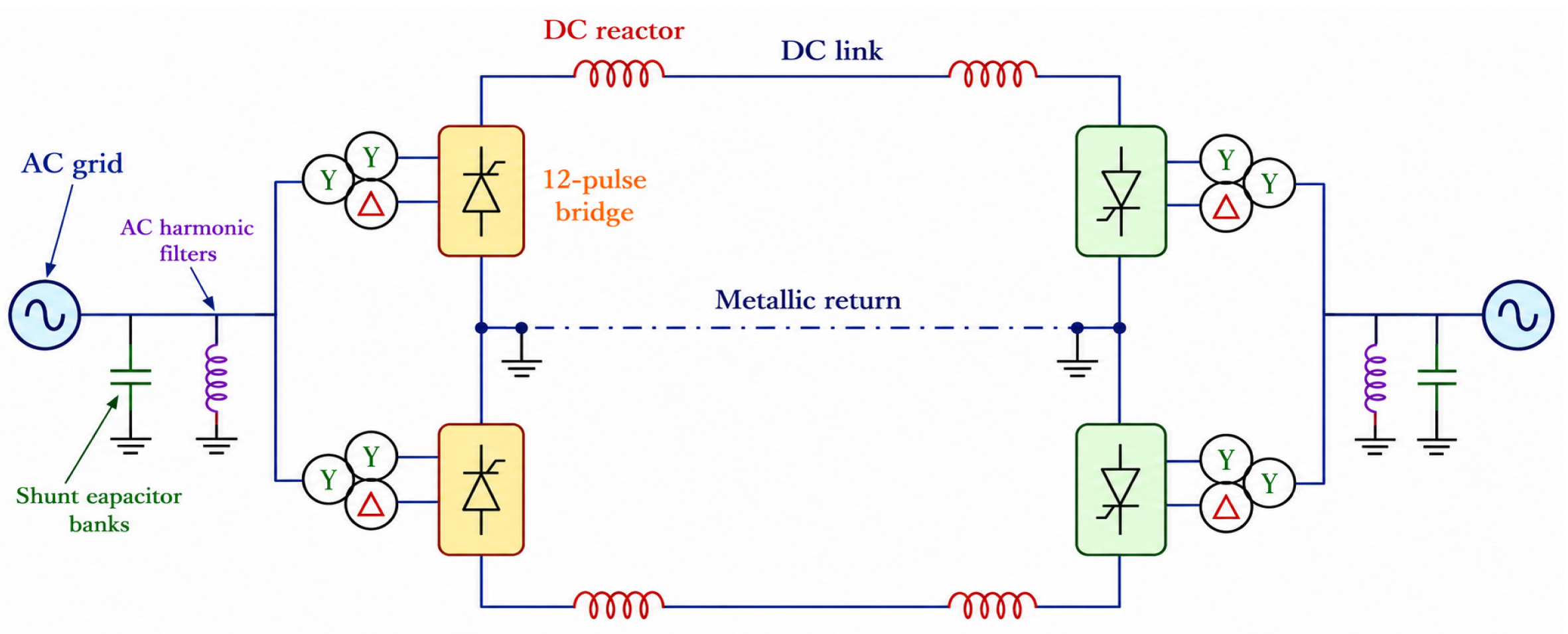
Thyristor-based LCC transmission can be utilized in a wide variety of power transmission applications, which include back-to-back interconnections between two asynchronous AC systems, power transfer via submarine or underwater cables, as well as long-distance overhead lines. For power transmission, we are able to utilize both monopole links (with ground return) and bipolar transmission links. Figure 1 depicts the LCC-HVDC system in bipolar structure, which includes AC filters, shunt capacitor banks or even other reactive-power compensating devices, converter transformers, converter stations, DC reactors, DC filters, as well as DC lines or cables, as discussed in Refs. [21,22,23].

Current Source Converters

LCC-HVDC systems rely on Line-Commutated Converters—specifically current-source converters (CSCs)—which require a stable AC voltage to function efficiently. Essentially, these converters switch AC power to DC at the transmission point and then convert it back to AC at the receiving end. While the system keeps the DC current steady, it controls the amount and direction of power flow by adjusting the DC voltage. The core component of this setup is the six-pulse Graetz bridge, which can send electricity in either direction. This is managed by changing the firing angles of the thyristor valves. If the angle is set below 90°, the bridge acts as a rectifier, moving energy from the AC side to the DC side. However, if the angle goes beyond 90°, the voltage polarity flips, and the system acts as an inverter, sending power from the DC side back to the AC side [24].

The six-pulse valve bridge is the fundamental converter unit, which can be combined either in series or in parallel to form the 12-pulse converter bridge. The bridges are linked to the AC grid using transformers with specific winding arrangements (Y-Y and Y-Δ). This configuration causes the 5th and 7th harmonic currents in the two transformers to cycle in opposite phases. Consequently, they cancel each other out, which greatly reduces harmonic distortion in the overall AC system [25].

5. Control System of LCC-HVDC Systems

5.1. LCC-HVDC Control Functions and Operation Modes

Under normal conditions, the rectifier end controls the DC current (${\mathrm{I}}_{\mathrm{d}\mathrm{c}}$) by operating in constant current control mode, whereas the inverter regulates the DC voltage (${\mathrm{V}}_{\mathrm{d}\mathrm{c}}$), controlling (${\mathrm{I}}_{\mathrm{d}\mathrm{c}}$ and ${\mathrm{V}}_{\mathrm{d}\mathrm{c}}$) to maintain the desired power transfer on the DC link. Therefore, it is necessary to continually measure the system quantities such as (${\mathrm{I}}_{\mathrm{d}\mathrm{c}}$, ${\mathrm{V}}_{\mathrm{d}\mathrm{c}}$, firing delay angle $\mathsf{\alpha }$, and inverter extinction angle $\mathsf{\gamma }$). Converters’ functions might reverse under abnormal operating conditions such as dropped AC voltage or fault cases. This is further detailed in the next section.

The normal mode of operation involves rectifier control, which is responsible for controlling the DC current (${\mathrm{I}}_{\mathrm{d}\mathrm{c}}$) through the use of constant current control mode, whereas the inverter control is used for controlling the DC voltage (${\mathrm{V}}_{\mathrm{d}\mathrm{c}}$). It can be said that the main purpose behind the control of (${\mathrm{I}}_{\mathrm{d}\mathrm{c}}$ and ${\mathrm{V}}_{\mathrm{d}\mathrm{c}}$) is maintaining the required level of power transmission over the DC link. It is therefore important to continuously measure all the parameters, including ${\mathrm{I}}_{\mathrm{d}\mathrm{c}}$, ${\mathrm{V}}_{\mathrm{d}\mathrm{c}}$, the firing angle $\mathsf{\alpha }$, and the extinction angle $\mathsf{\gamma }$ of the inverter under any conditions. It should be noted that the roles of the converters can change during abnormal operations, including situations where there is a drop in AC voltage or any faults occur. This aspect will be explained in more detail in the next section [21,26].

5.1.1. Rectifier Control Mode

The rectifier of the LCC-HVDC system usually runs in constant current control mode; besides, it can also be switched to constant firing angle mode.

(a) 

Constant Current Control:

The rectifier controller continuously adjusts the firing angle $\mathsf{\alpha }$ to maintain DC current (${\mathrm{I}}_{\mathrm{d}\mathrm{c}}$) at reference value (${\mathrm{I}}_{\mathrm{o}\mathrm{r}\mathrm{d}\mathrm{e}\mathrm{r}}$), usually between ${15}^{\circ }<\mathsf{\alpha }<{18}^{\circ }$ to provide proper voltage. If the DC line resistance increases or the inverter voltage rises, the rectifier decreases $\mathsf{\alpha }$ (closer to $0^{\circ }$) to increase its output voltage and feed the needed current through the link.

(b) 

Constant Firing Angle:

However, the rectifier’s voltage is capable of being increased until the firing angle approaches $\mathsf{\alpha }=2$, which is the minimum limit needed to ensure that t the thyristors have a positive forward voltage across them before triggering. Once the controller hits $\mathsf{\alpha }=2^{\circ }$, it cannot increase the DC voltage to maintain current flow. In this case, the rectifier switches into constant firing angle mode ($\mathsf{\alpha }=\mathrm{c}\mathrm{o}\mathrm{n}\mathrm{s}\mathrm{t}\mathrm{a}\mathrm{n}\mathrm{t}$). If the system demand needs additional voltage, the DC current will naturally gradually drop because the rectifier has reached its maximum operational range. The reason for choosing $\mathsf{\alpha }=2^{\circ }$ rather than $0^{\circ }$ is that selecting $\mathsf{\alpha }=0^{\circ }$ mathematically delivers the maximum voltage. A little firing angle (such as $\mathsf{\alpha }=2^{\circ }$) is kept in real HVDC systems to ensure a reliable firing of all thyristors in a bridge and provide a small margin for control stability.

5.1.2. Inverter Control Mode

There are three different modes of operation for the inverter based on the system condition; these modes are listed below [21]:

(a) 

Operation Under Normal Conditions:

The inverter works under a constant DC voltage (${\mathrm{V}}_{\mathrm{d}\mathrm{c}}$) control mode so as to keep the system stable, whereas the rectifier will maintain control over the DC current (${\mathrm{I}}_{\mathrm{d}\mathrm{c}}$).

(b) 

AC Voltage Drops at the Rectifier Side:

Whenever there is a voltage drop, the rectifier lowers its firing angle so as to reduce the voltage drop until the firing angle reaches its limit. Thereafter, the rectifier switches to constant firing angle control mode ($\mathsf{\alpha }=\mathrm{c}\mathrm{o}\mathrm{n}\mathrm{s}\mathrm{t}\mathrm{a}\mathrm{n}\mathrm{t}$). Meanwhile, the inverter runs in a constant DC current (${\mathrm{I}}_{\mathrm{d}\mathrm{c}}$) mode, whereby it operates in constant current control mode and reduces the reference current (${\mathrm{I}}_{\mathrm{r}\mathrm{e}\mathrm{f}}$) using the current margin (${\mathrm{I}}_{\mathrm{m}\mathrm{a}\mathrm{r}\mathrm{g}\mathrm{i}\mathrm{n}}$). This implies that there is always about 10–15% margin between order currents (${\mathrm{I}}_{\mathrm{o}\mathrm{r}\mathrm{d}\mathrm{e}\mathrm{r}}$) in the rectifier and in the inverter stations so that they do not compete against each other.

(c) 

AC Voltage Drops at the Inverter Side:

When there is a voltage drop on the inverter side, the rectifier continues to control the DC current (${\mathrm{I}}_{\mathrm{d}\mathrm{c}}$) whereas the inverter operates under constant extinction angle control mode to avoid commutation failure.

The overall conclusion from the above discussion is that the LCC-HVDC technology cannot be used for ensuring the transmission of the rated DC current (${\mathrm{I}}_{\mathrm{d}\mathrm{c}}$) in case the AC voltage drops beyond 25 percent. This is because, with the decreasing voltage on the AC side, the firing angle of the rectifier would approach its minimum value in order to restore the voltage losses. The further decrease in AC voltage will cause the rectifier to shift into the constant control mode while the inverter maintains (${\mathrm{I}}_{\mathrm{d}\mathrm{c}}$) at a lower level. Since neither the rectifier nor the inverter controls (${\mathrm{V}}_{\mathrm{d}\mathrm{c}}$), it may be subjected to further reductions in value. For this reason, the Voltage Dependent Current Order Limiter (VDCOL) mode of control is developed for limiting the maximum DC current allowed during voltage reductions beyond certain levels. It should be noted that the characteristics of VDCOL can depend on the DC voltage (${\mathrm{V}}_{\mathrm{d}\mathrm{c}}$) or the AC commutation voltage. The three control modes were designed in order to provide stability of the DC system and minimize its reactive power usage due to the fact that large firing or extinction angles result in large amounts of reactive power consumption [26].

5.2. Hierarchical Control System for LCC-HVDC Link

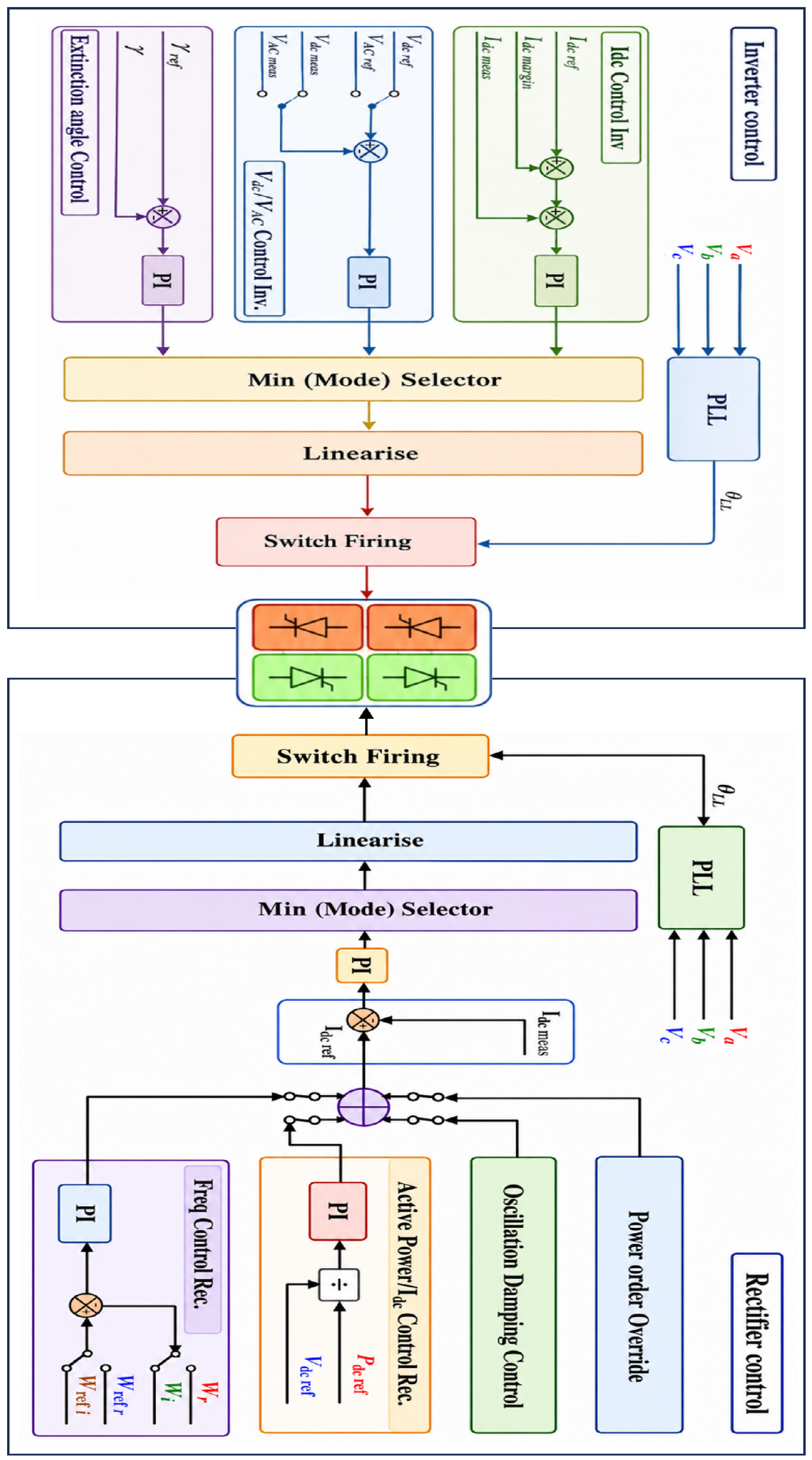
The hierarchical control scheme for an LCC-HVDC link has been schematically represented in Figure 2. In the case of a bi-directional HVDC interconnection system, both the inverter and rectifier are able to switch their operating modes quickly. Three different modes of operation exist for an inverter, namely, constant DC voltage control/constant AC voltage control, constant extinction angle (CEA), and constant current control. Constant extinction angle is essential to avoid any kind of commutation failures; hence, CEA is considered the main control mode of operation for inverters. However, in some instances, this mode of control might not provide sufficient stability due to disturbances or owing to a weak AC tie line associated with the DC transmission system. In such situations, DC and AC voltage control will serve as the main control mode at the inverter end [21].

The (${\mathrm{I}}_{\mathrm{d}\mathrm{c}}$) control or active power control is not active in normal operating conditions; nevertheless, the importance of this backup control function comes out in case of failure occurring in the DC part or failure in the (${\mathrm{I}}_{\mathrm{d}\mathrm{c}}$) control of the rectifier because of a drop in the AC voltage across the rectifier. Constant Current Control Function in the Inverter is performed by comparing the desired current (${\mathrm{I}}_{\mathrm{o}\mathrm{r}\mathrm{d}\mathrm{e}\mathrm{r}}$) to the reference current (${\mathrm{I}}_{\mathrm{r}\mathrm{e}\mathrm{f}}$).

Figure 2 shows the concept of master level hierarchical control for the rectifier side, which provides the reference value for current (${\mathrm{I}}_{\mathrm{r}\mathrm{e}\mathrm{f}}$) to the primary DC current controller. The rectifier plays an active role in power regulation by estimating the DC power at the reference value for DC voltage along with generating order current (${\mathrm{I}}_{\mathrm{o}\mathrm{r}\mathrm{d}\mathrm{e}\mathrm{r}}$) [26].

Figure 2 shows the implementation of frequency control and power oscillation damping on the rectifier side. Power oscillation damping can enhance the stability of the network in case of badly damped oscillations, and this signal is usually fed into (${\mathrm{I}}_{\mathrm{o}\mathrm{r}\mathrm{d}\mathrm{e}\mathrm{r}}$). Along with this, an active power order override is offered for employing in post-fault operations and other events. The firing angle is established by all three controllers, and the firing pulses for the inverter valves are determined by selecting the lowest output from these controllers via select minimum Gamma angle. The firing angles are limited to the range of ${110}^{°}$ to ${170}^{°}$, so as to avoid commutation failure or accidental switching to rectification mode [19,21,26].

6. Limitations of LCC-HVDC Systems

Due to the following limitations, the LCC-HVDC system is considered inefficient; thus, restricting its application range [3,18,22].

(a)

Voltage distortions on the AC side can cause commutation failures and interruptions in power transmission. Thus, in the conventional HVDC system, the rectifier and inverter require a sufficiently strong AC network to ensure valve commutation. The thing is, LCC requires an even more powerful receiving network than an HVDC link.

(b)

The presence of multiple terminals causes at least two kinds of problems. First, active power flow reversal requires DC polarity reversal. Second, fast communication between all terminals is necessary due to control needs.

(c)

Reactive power has to be compensated by external sources, mostly by means of switching filters and other capacitor banks.

(d)

LCC-HVDC systems lack black start capability. They cannot provide power to the network without other generation sources.

(e)

Limited control bandwidth for AC voltage and reactive power, potentially impacting wind turbine generator (WTG) stability and grid compatibility.

(f)

Continuous operation at active power levels below 5% may be impossible, making it difficult for the wind plant to operate at low wind speeds.

Therefore, VSC-HVDC is introduced to deal with the drawbacks of LCC-HVDC.

7. VSC-HVDC Configurations

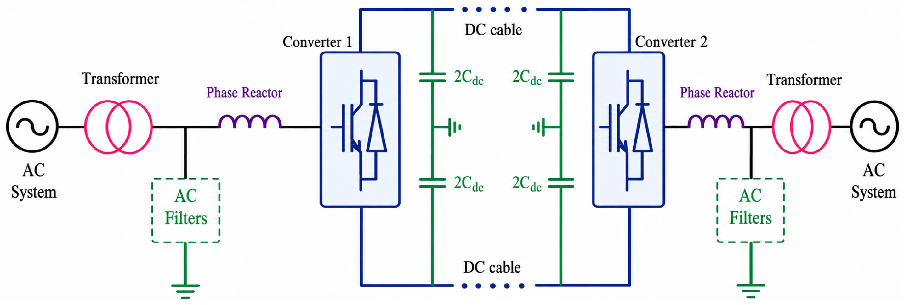
Figure 3 demonstrates the standard structure of a VSC-HVDC transmission system.

This transmission system comprises two Voltage Source Converters, transformers, phase reactors, AC filters, DC-link capacitors, and DC cables. The Refs. [24,27,28] described each of these components in detail.

Voltage Source Converter

Both Voltage Source Converters (VSCs) make up the main parts of the HVDC transmission system, whereby one acts as a rectifier while the other acts as an inverter, both utilizing power semiconductors made using IGBT technology. Generally, there are mainly three types of VSCs that can be used in HVDC transmissions: the two-level converters, the three-level converters, and the modular multilevel converter. As stated above, the IGBT is basically a one-way switch and cannot conduct any current backward. This problem is resolved by placing an anti-parallel diode together with the IGBT [24].

The two-level converter is the easiest topology available for HVDC transmission. The converter consists of a six-pulse bridge made of IGBTs with anti-parallel diodes, which can produce two levels of voltages (−1/2 V_dc and +1/2 V_dc) on the AC side [24,29].

The three-level VSC configuration is an alternative to the two-level VSC configuration in high-power applications because the phase can be varied between three levels of voltage on the AC side of the converter (−1/2 Vdc, 0, +1/2 Vdc) and obtain low harmonics without increasing switching losses. In such an arrangement, the converter arm is composed of four valves [24]. The structure and output waveforms of the two-level and three-level converters are depicted in Ref. [29].

The modular multilevel converter (MMC) consists of six valves in three submodules, similar to the two-level converter. The valves are linked from one DC terminal to one AC terminal, which is similar to the two-level converter [30]. Where it differs is that each valve in the MMC acts as a controllable voltage source equipped with its own dedicated storage capacitor. Inside each submodule(SM), two IGBTs are wired in series across this capacitor, and their middle junction connects directly to the AC voltage source. The structure and output waveforms of the two-level and three-level converters are depicted in Ref. [29].

MMCs offer significant advantages for VSC-HVDC systems, including excellent harmonic performance without the need for filters or PWM, as well as lower power losses than two-level converters. These benefits have made the MMC the dominant VSC technology in use today. However, there are some drawbacks, including a highly complex control system that requires heavy computing and high-speed communication between the central controller and the valves. Furthermore, the capacitors housed within each submodule make the physical size of an MMC much larger, demanding significantly more substation space [30,31].

8. Operational Principles of VSC-HVDC

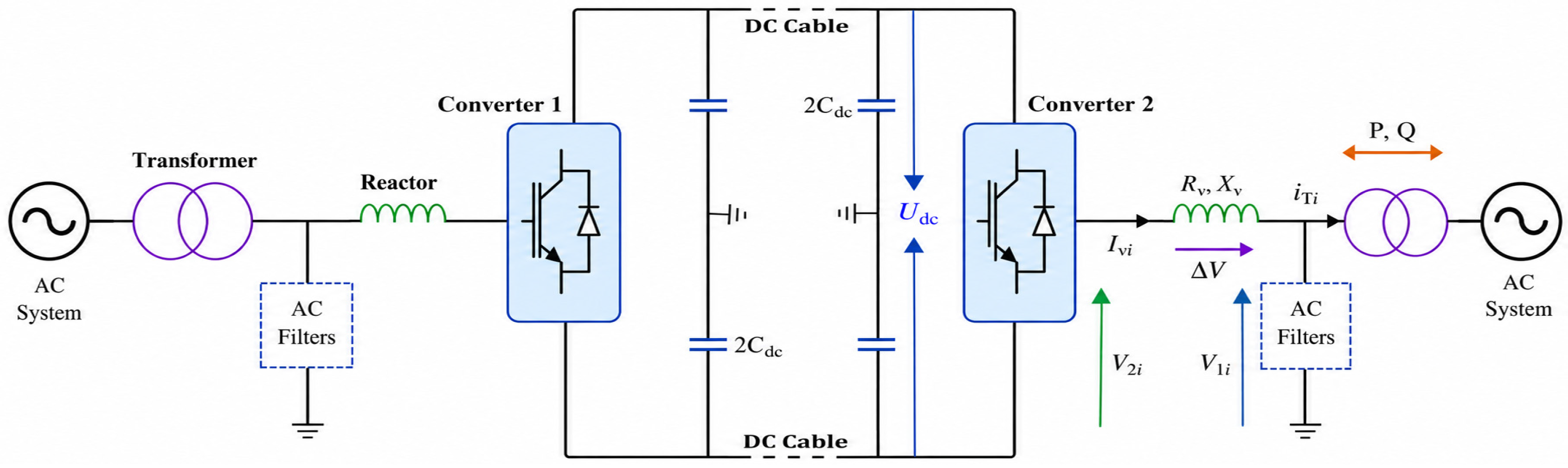
The basic operating principle of a VSC-based HVDC system may be described on the assumption that each terminal behaves like a voltage source that is connected to the AC grid via a series reactor. The DC link connecting two terminals is depicted in Figure 4 [22].

The converter is described as a controllable variable AC voltage source allowing control over the variables: amplitude, phase, and frequency. Therefore, the VSC bridge acts as a fast and effective synchronous machine, where the instantaneous phase voltage (${\mathrm{V}}_{2\mathrm{i}}$) is given by Equation (15) [22,32,33]:

$${\mathrm{V}}_{2\mathrm{i}}={\displaystyle \frac{1}{2}}{\mathrm{U}}_{\mathrm{d}\mathrm{c}}\mathrm{M}\sin \left(\mathsf{\omega }\mathrm{t}+\mathrm{\phi }\right)+\mathrm{h}\mathrm{a}\mathrm{r}\mathrm{m}\mathrm{o}\mathrm{n}\mathrm{i}\mathrm{c} \mathrm{t}\mathrm{e}\mathrm{r}\mathrm{m}\mathrm{s}$$

(15)

where $\mathrm{M}$ is the modulation index (peak value of modulating wave/peak value of carrier wave), $\mathsf{\omega }$ is the fundamental frequency. $\mathrm{\phi }$ is the output voltage phase shift, and ${\mathrm{U}}_{\mathrm{d}\mathrm{c}}$ is the DC link voltage.

8.1. Power Flow Control

By manipulating the variables (M) and ($\mathrm{\phi }$), the VSC controller can independently vary the voltage magnitude and phase shift relative to the fundamental-frequency voltage in the AC network. Controlling the voltage drop ($∆\mathrm{V}$) across the reactor (${\mathrm{X}}_v$) (see Figure 4) is necessary for controlling the active and reactive power flows [22,32,33].

8.1.1. Active Power Control (P)

The phase difference ($\mathrm{\phi }$) between the fundamental voltage generated by VSC (${\mathrm{V}}_{2\mathrm{i}}$) and bus voltage (${\mathrm{V}}_{1\mathrm{i}}$) is used to manipulate the active power flow. For determining the active power, Equation (16) is utilized without taking into consideration losses in the reactor (${\mathrm{X}}_v$).

$$\mathrm{P}={\displaystyle \frac{{\mathrm{V}}_{2\mathrm{i}} {\mathrm{V}}_{1\mathrm{i}} \sin \phi }{{\mathrm{X}}_v}}$$

(16)

8.1.2. Reactive Power Control (Q)

Varying the magnitude of ${\mathrm{V}}_{2\mathrm{i}}$ which depends on Pulse Width Modulation (PWM), enables control of reactive power. The reactive power flow is determined from Equation (17):

$$\mathrm{Q}={\displaystyle \frac{{\mathrm{V}}_{2\mathrm{i}} ({\mathrm{V}}_{2\mathrm{i}}-{\mathrm{V}}_{1\mathrm{i}} \cos \phi )}{{\mathrm{X}}_v}}$$

(17)

8.2. Operational Modes (Rectifier vs. Inverter)

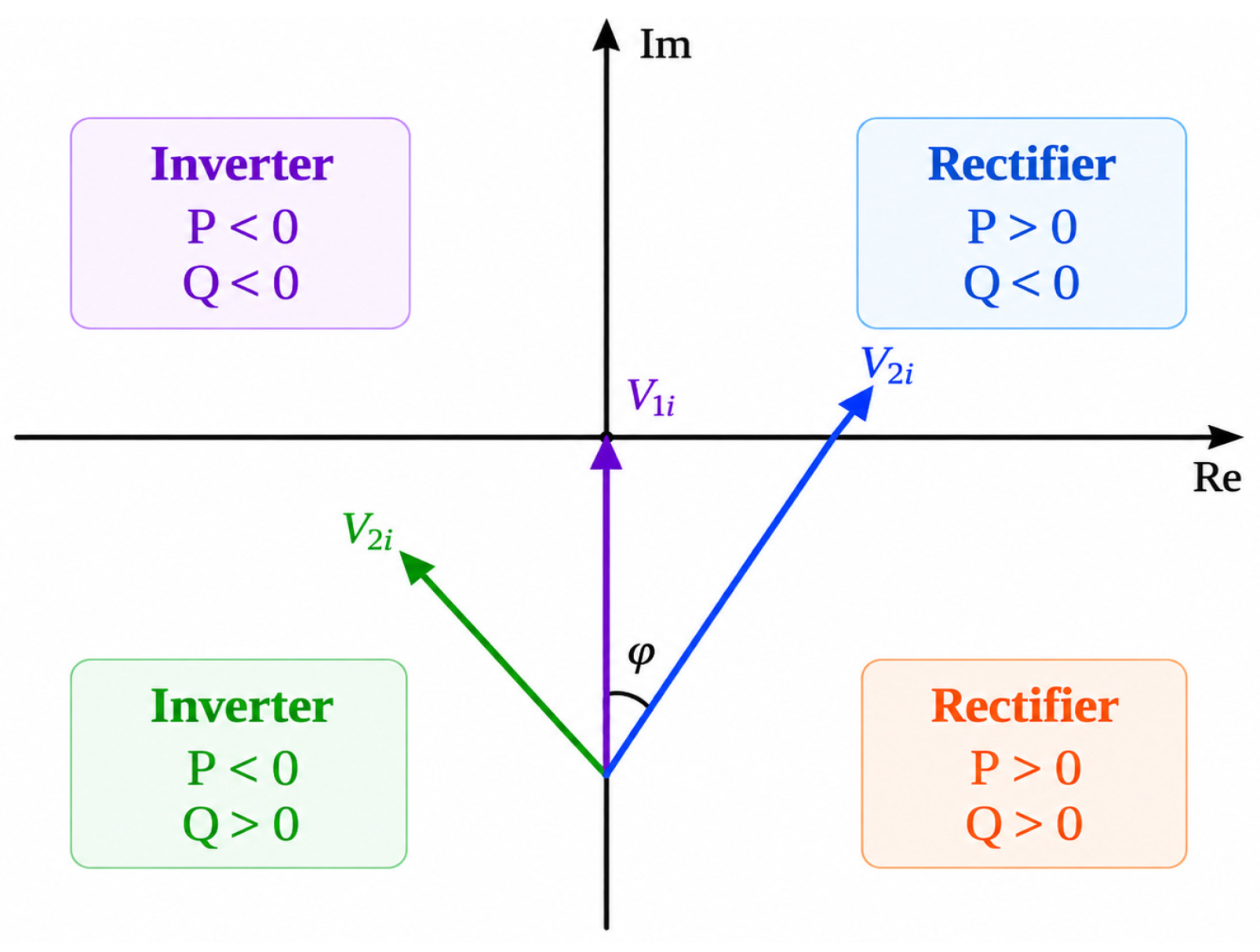
The operational mode of a Voltage Sourced Converter (rectifier or inverter) depends largely on the relative position between the voltage phasor of the converter (${\mathrm{V}}_{2\mathrm{i}}$) and that of the AC system bus (${\mathrm{V}}_{1\mathrm{i}}$). Based on the phasor orientation, there are two operation modes as discussed in Figure 5:

(a)

Rectifier Mode ($\mathbf{P}>0$): Active power is flowing from the AC system grid to the converter station in cases where the line voltage (${\mathrm{V}}_{1\mathrm{i}}$) leads the bridge voltage (${\mathrm{V}}_{2\mathrm{i}}$).

(b)

Inverter Mode ($\mathbf{P}<0$): Active power is flowing from the converter station to the AC network in cases where the bridge voltage (${\mathrm{V}}_{2\mathrm{i}}$) leads the line voltage (${\mathrm{V}}_{1\mathrm{i}}$) [22].

8.3. Power Flow Balance

In steady state, the amount of active power delivered on the AC side will be equivalent to that delivered from the DC side (ignoring losses). This balance is established through the collaboration of two converters; one controlling the active power and the other responsible for maintaining the DC link voltage between specific values. On the other hand, on the AC side, the voltage will be regulated at both ends based on the AC voltage reference value utilizing cos (φ) or by a chosen reactive power control strategy. Reactive power generation is used to compensate for the demands of the linked AC network.

9. Hierarchical Control Architecture of VSC-HVDC System

In the context of modern VSC-HVDC control, it is essential to distinguish between two fundamental paradigms of grid interaction: Grid-Following (GFL) and Grid-Forming (GFM) control. The advanced control and optimization strategies reviewed in the subsequent sections of this manuscript—such as Variable Coefficient PI, Fuzzy PI, and Model Predictive Control—are primarily developed and evaluated within the traditional Grid-Following framework. In this paradigm, the VSC operates as a controlled current source that relies on a Phase-Locked Loop (PLL) to synchronize with, and track, the fundamental frequency and voltage phase established by the host AC grid. This GFL approach remains the standard and highly effective control structure for conventional point-to-point HVDC transmission systems interconnected with synchronous generation [34].

Conversely, Grid-Forming control represents a distinct paradigm shift where the converter emulates the behavior of a synchronous machine, acting as a controlled voltage source capable of independently establishing grid voltage and frequency without relying on a PLL. This approach typically incorporates specialized topologies such as Virtual Synchronous Machines (VSM), droop-based control, or virtual oscillator control. GFM technology is of critical and growing importance, particularly for integrating HVDC systems into converter-dominated, low-inertia, or passive AC networks [35].

However, a detailed structural review of dedicated GFM topologies requires a substantially broader treatment of inverter-dominated grid dynamics that falls outside the defined scope of the present study. Therefore, while GFM control is acknowledged here as a vital emerging research direction for future HVDC applications, the comparative analysis in this review focuses rigorously on optimizing the standard cascaded GFL control loops. The emphasis remains on demonstrating how advanced tuning methodologies can enhance the robustness, disturbance rejection, and dynamic performance of traditional point-to-point VSC-HVDC systems under varying grid strengths [36].

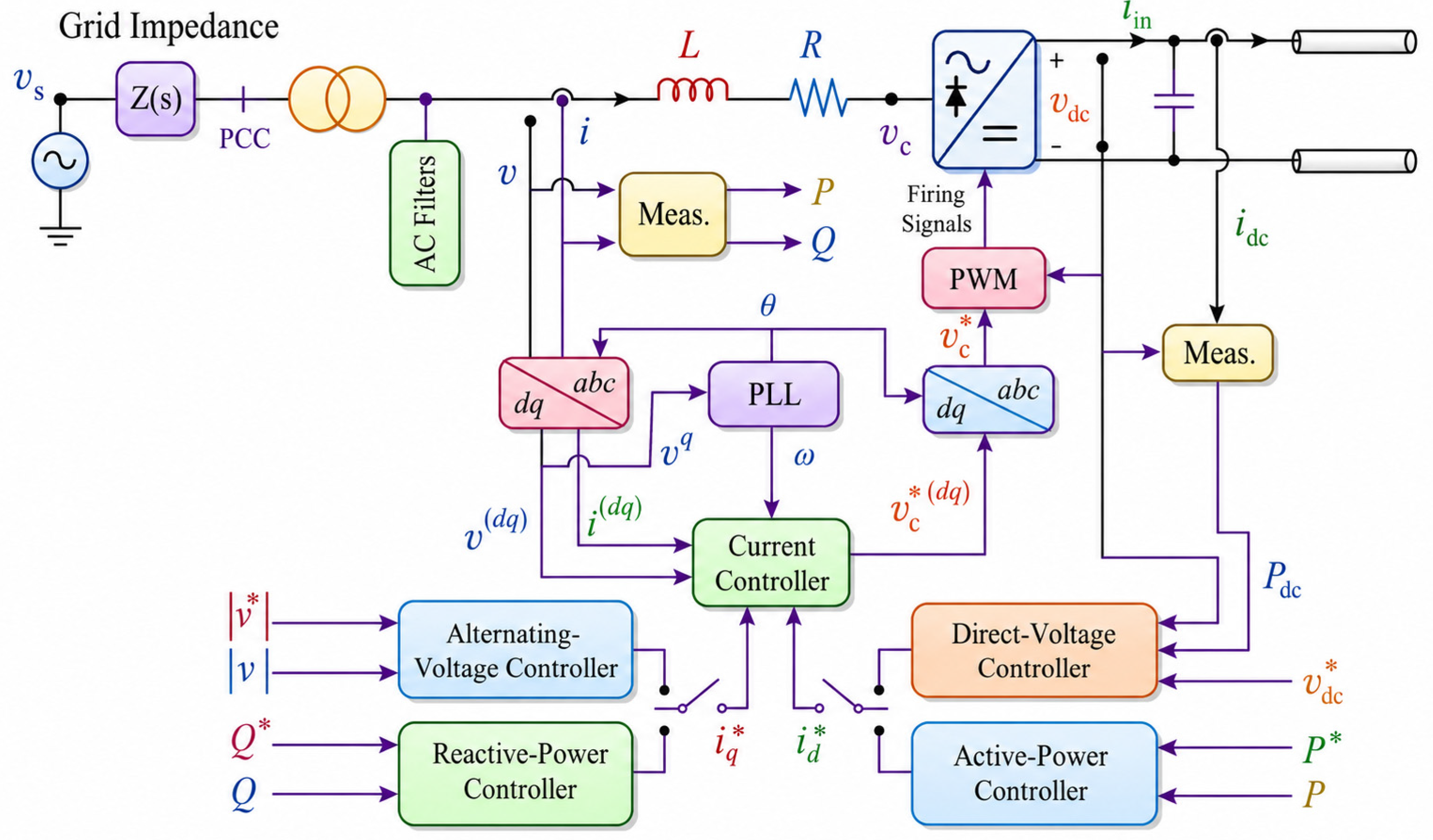
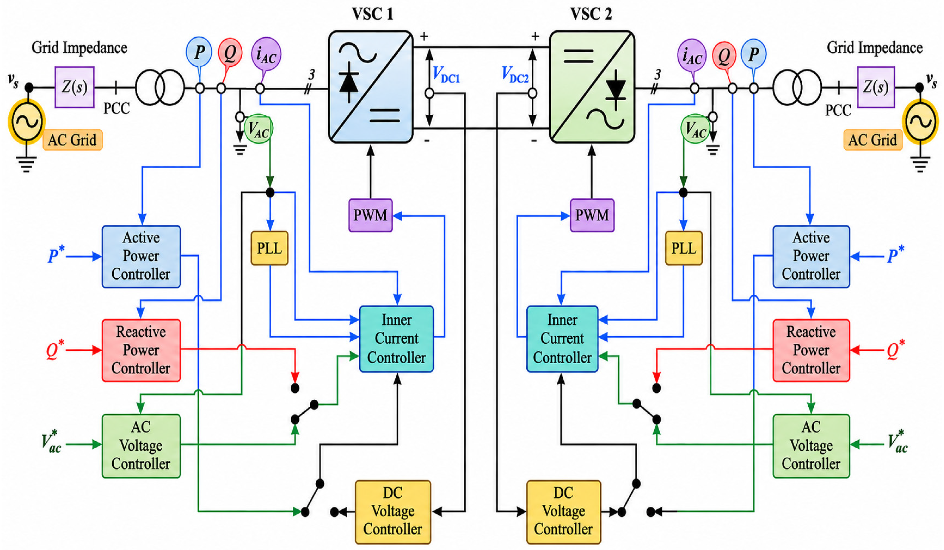
The VSC-HVDC control system uses a hierarchical architecture and is structured into cascaded layers that operate across multiple timescales. This multilayer design enables accurate control of power flow and voltage regulation and keeps system stability under both steady-state and dynamic conditions. As shown in Figure 6, the fundamental concept in controlling VSC-HVDC lies in vector control. The vector control technique makes it possible to separately control active and reactive power by converting three-phase AC signals into a rotating dq axis system. By doing so, independent control of active (d-axis) and reactive power (q-axis) becomes feasible using PI regulators [37,38].

This cascaded (hierarchical) control structure shown in Figure 6 consists of [37]:

(a)

Supervisory Control (bandwidth < 5 Hz): This top layer manages the complete system, handling inter-station communications, power flow control, and operational mode control. Response time typically ranges from 0.2 to 2 s. At this lowest frequency, there is continual interaction with SCADA systems. Output of the supervisory control includes set-points of the active power ($P^{*}$), reactive power ($Q^{*}$), DC voltage ($V_{dc}^{*}$), and the AC voltage magnitude ($V_{ac}^{*}$).

(b)

Outer Control Loops (bandwidth 5 to 50 Hz): This group of loops implements control at a lower speed but with wider control goals covering DC voltage, active power, frequency, reactive power, and AC voltage control. Response time in this case ranges from 20 to 200 milliseconds. The output of these controllers includes reference currents ($i_d^{*}$ and $i_q^{*}$) that will be provided to the next inner control loops.

(c)

Inner Current Control Loops (bandwidth 200 to 500 Hz): At this layer of control, AC current regulation is carried out with the help of high-speed Proportional–Integral (PI) controllers whose response time is within the 1 to 5 millisecond range. In this way, accurate tracking by the converter of the reference currents is ensured. Current references ($i_d^{*}$ and $i_q^{*}$) calculated at the outer layers are correctly transformed into the converter reference voltage ($v_d^{*}$ and $v_q^{*}$) via inner control. The controller’s outputs are the converter reference voltages ($v_d^{*}$ and $v_q^{*}$).

(d)

Bridge Level Control (Zero-Level Control): The lowest level control in the VSC-HVDC hierarchy utilizes the continuous voltage references ($v_d^{*}$ and $v_q^{*}$) generated from the inner loop and transforms them back to the abc phase frame (via inverse Park transformation), then generates discrete high-frequency (ON/OFF) firing pulses for the IGBTs using Sinusoidal Pulse Width Modulation (SPWM). The response time range is nanoseconds to microseconds.

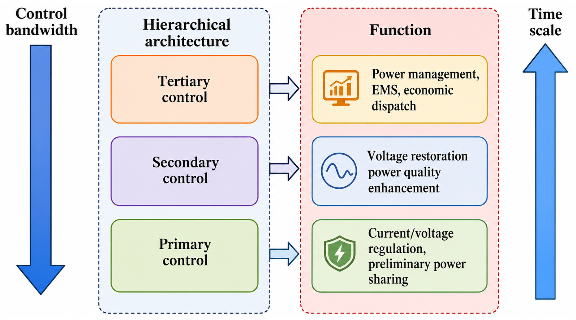
The above-discussed multi-layered control architecture enables efficient operation of VSC-HVDC transmission lines in various dynamic situations encountered in power grids. Figure 7 provides an illustration of the hierarchical approach, which includes primary control responsible for control of converters, secondary control for steady-state restoration, and tertiary control for supervision of the whole system.

This hierarchical control technique makes it possible to perform different control tasks in each layer according to its own dynamics. Such an organization of the controller enables fast responses to sudden electrical events while at the same time implementing slower operations such as power flow and voltage controls [37].

10. Operational Modes of VSC-HVDC and AC Grid Conditions

10.1. Primary Operating Modes of VSC-HVDC

The flexible control ability of VSC-HVDC systems allows operation in several modes, depending on the conditions of the grid and needs of the system. This is due to the possibility of individual control of the active and reactive power of the converter. A VSC-HVDC converter can have five different operational modes [21,39]:

• Active and Reactive Power Control: In this fundamental mode of the converter, setpoints for active and reactive power are provided by the operator, and the real-time switching sequence of the converter’s valves is continuously adjusted to ensure power transmission within the allowed range (usually with an error no more than 1% of rated). The mode allows planning power transmissions, e.g., participation in a day-ahead market or interregional power transmission.
• DC Voltage and Reactive Power Control: In this scenario, one converter controls the DC voltage, whereas another converter is responsible for the transmission of (control) active power. All converters control reactive power on AC terminals. This mode is used in point-to-point HVDC networks and forms the basis of more advanced multi-terminal HVDC networks.
• AC Voltage and Active Power Control: This mode should be used in case the stabilization of AC voltage at the converter site becomes necessary. The converter controls AC voltage by setting appropriate reactive power and controlling active power to a predetermined setpoint level. This combination allows uninterruptible power transmission while supporting voltage regulation. Due to the possible interference between the control of active and reactive powers, special control methods have been developed to ensure stability.
• Frequency and Reactive Power Control: The frequency of the connected AC network is regulated in this mode. The power transmitted from the converter is controlled following the droop curve, i.e., power decreases with increasing frequency and increases when frequency falls. Such mode of operation resembles that of synchronous generators, providing higher stability.
• Black Start (Frequency and AC Voltage Control): Black start is a special operational mode, during which a converter of VSC-HVDC provides a startup of a disconnected part of the AC network. In contrast to conventional HVDC converters, VSCs work as voltage sources and provide uninterruptible transmission of three-phase AC voltage with controlled frequency, even without connection to the main AC network. This allows restoring the power supply by providing voltage to other components of the system, such as transformers and ancillary equipment. In this case, the control system should handle considerable inrush currents while maintaining voltage stability, usually by adopting advanced forms of control and limiting the amount of initial generated power. With more elements being energized within the power system, the power electronics converter may transition into other modes of operation, such as active and reactive power regulation.

10.2. Typical Operating Control Mode Combinations of VSC-HVDC

Active and reactive power regulation takes place at both ends of the DC link (rectifier and inverter). However, not all the controllers can be enabled and used simultaneously; the application determines which control functionalities are used. In the case of a passive load, it is required that the converter regulates frequency and voltage, but in the case of a strong AC system (or reactive power), the converter regulates voltage and active power. In any case, the regulation of DC voltage becomes necessary for achieving balance in active power of the DC link. Therefore, at one end of the DC link it will regulate the DC voltage, while on the other end, it will regulate the active power or frequency. As far as the reactive power regulation is concerned, both types of control modes may be enabled independently of each other on both ends of the DC link, as indicated in Figure 6 [5,24].

Table 2 outlines the various operational configurations for VSC and HVDC.

Table 2. Operating control mode combinations of VSC- HVDC.

Case	VSC1 (Rectifier)		VSC2 (Inverter)
	Controller-(1)	Controller-(2)	Controller-(1)	Controller-(2)
1	Active Power	Reactive Power	DC Voltage	Reactive Power
2	Active Power	AC Voltage	DC Voltage	AC Voltage
3	DC Voltage	Reactive Power	Active Power	Reactive Power
4	DC Voltage	AC Voltage	Active Power	AC Voltage
5	Frequency	Reactive Power	DC Voltage	Reactive Power
6	Frequency	AC Voltage	DC Voltage	AC Voltage
7	DC Voltage	Reactive Power	Frequency	Reactive Power
8	DC Voltage	AC Voltage	Frequency	AC Voltage

Table 2. Operating control mode combinations of VSC- HVDC.

Case	VSC1 (Rectifier)		VSC2 (Inverter)
	Controller-(1)	Controller-(2)	Controller-(1)	Controller-(2)
1	Active Power	Reactive Power	DC Voltage	Reactive Power
2	Active Power	AC Voltage	DC Voltage	AC Voltage
3	DC Voltage	Reactive Power	Active Power	Reactive Power
4	DC Voltage	AC Voltage	Active Power	AC Voltage
5	Frequency	Reactive Power	DC Voltage	Reactive Power
6	Frequency	AC Voltage	DC Voltage	AC Voltage
7	DC Voltage	Reactive Power	Frequency	Reactive Power
8	DC Voltage	AC Voltage	Frequency	AC Voltage

10.3. Grid Classification and Operating Control Modes Selections

Definition of Grid Strength: The strength of an AC grid at the point of common coupling (PCC) of a VSC-HVDC terminal is quantified by the Short-Circuit Ratio (SCR), defined as the ratio of the short-circuit apparent power of the AC bus ($S_{SC}$, in MVA) to rated DC power ($P_{DC}$, in MW) [40]:

$$SCR = S_{SC}/P_{DC}$$

(18)

A high SCR indicates that the AC bus has a large fault level relative to the converter power, meaning its voltage is stiff and largely unaffected by disturbances. Conversely, a low SCR implies high coupling impedance: any change in active or reactive power injection causes a proportionally large voltage deviation, making the AC bus inherently volatile [41,42].

Table 3 summarizes the four practical grid categories, their SCR ranges, key electrical characteristics, and the corresponding control strategy required at the VSC-HVDC terminal. While these SCR thresholds (e.g., very strong, strong, and weak) provide a highly useful foundational framework for designing and selecting control strategies, it is critical to recognize that they function as approximate engineering guidelines rather than strict, universally applicable physical limits [43,44,45,46,47].

Table 3. AC grid strength classification and VSC-HVDC control mode selections.

Grid Category	SCR Range	Electrical Characteristics	VSC-HVDC Control Modes
Very Strong Grid	SCR > 5	High short-circuit capacity; bus voltage is stiff and largely unaffected by reactive power variations. Abundant rotating inertia provides a stable frequency reference.	Active power and reactive power scheduling (Cases 1, 3) are sufficient. AC-voltage regulators are not required because the bus is inherently stiff.
Strong Grid	3 ≤ SCR ≤ 5	Adequate short-circuit level; voltage is generally stable but may respond to large reactive disturbances. Frequency is well-anchored by synchronous generation.	Standard operating modes apply (Cases 1–4). Reactive-power scheduling is acceptable; AC-voltage control may be selected as a precaution during heavy loading.
Weak Grid	2 ≤ SCR < 3	High coupling impedance causes the bus voltage to fluctuate significantly with reactive power changes. Voltage instability is a real risk under variable loading.	AC-voltage regulation replaces reactive-power scheduling (Cases 2, 4, 6, 8). Closed-loop voltage control is necessary to prevent PCC voltage violations.
Very Weak/ Passive Network	SCR < 2 or No Generation	Negligible or zero short-circuit capacity. No synchronous machines to establish frequency. Bus voltage is entirely dependent on the converter’s output.	Frequency control is mandatory (Cases 5–8). The converter operates in Grid-Forming mode, synthesizing both voltage and frequency entirely on its own.

Table 3. AC grid strength classification and VSC-HVDC control mode selections.

Grid Category	SCR Range	Electrical Characteristics	VSC-HVDC Control Modes
Very Strong Grid	SCR > 5	High short-circuit capacity; bus voltage is stiff and largely unaffected by reactive power variations. Abundant rotating inertia provides a stable frequency reference.	Active power and reactive power scheduling (Cases 1, 3) are sufficient. AC-voltage regulators are not required because the bus is inherently stiff.
Strong Grid	3 ≤ SCR ≤ 5	Adequate short-circuit level; voltage is generally stable but may respond to large reactive disturbances. Frequency is well-anchored by synchronous generation.	Standard operating modes apply (Cases 1–4). Reactive-power scheduling is acceptable; AC-voltage control may be selected as a precaution during heavy loading.
Weak Grid	2 ≤ SCR < 3	High coupling impedance causes the bus voltage to fluctuate significantly with reactive power changes. Voltage instability is a real risk under variable loading.	AC-voltage regulation replaces reactive-power scheduling (Cases 2, 4, 6, 8). Closed-loop voltage control is necessary to prevent PCC voltage violations.
Very Weak/ Passive Network	SCR < 2 or No Generation	Negligible or zero short-circuit capacity. No synchronous machines to establish frequency. Bus voltage is entirely dependent on the converter’s output.	Frequency control is mandatory (Cases 5–8). The converter operates in Grid-Forming mode, synthesizing both voltage and frequency entirely on its own.

The actual suitability and dynamic stability of an HVDC installation—whether LCC-HVDC or VSC-HVDC—for a particular AC system cannot be accurately reduced to a single numerical SCR value. Instead, the true system strength and the resulting control challenges depend on a complex interplay of multiple system-specific variables. The reliability of the classifications presented in Table 3 is heavily influenced by factors including [43,44,45,46,47]:

•

Network Topology and Capacity: The specific physical layout of the surrounding grid and the localized short-circuit capacity at the point of common coupling (PCC).

•

Impedance Characteristics: The local commutation reactance (particularly critical for LCC systems) and the harmonic impedance profile of the interconnected network.

•

Voltage Dynamics: The dynamic AC voltage characteristics, including the magnitude and rate of voltage fluctuations during transient disturbances.

•

Control Interactions: Complex electromagnetic and electromechanical control interactions between the HVDC converter and the grid’s existing voltage regulation mechanisms.

•

Nearby Converter-Interfaced Resources (CIRs): The presence of renewable energy sources (like wind or solar farms) near the PCC, which fundamentally alter traditional fault-current behaviors and reduce effective inertia.

•

Operating Conditions: The real-time loading scenarios, power flow directions, and specific operational states of the grid at the time of a disturbance.

•

Multi-Converter Interactions: In multi-infeed HVDC configurations, the electrical proximity and adverse interactions between multiple converters, which can artificially depress the effective grid strength perceived by any single terminal.

Accordingly, the control mode selections suggested in Table 3 should be viewed as baseline starting points derived from common engineering practice and literature. In modern power systems, where the factors listed above are highly variable, the definitive boundaries between “strong” and “weak” grids become increasingly blurred. This reality underscores the primary motivation of this review: the necessity for advanced, adaptive, and robust control strategies that can maintain stability even when simplistic SCR-based guidelines are insufficient to guarantee reliable operation.

10.4. VSC-HVDC Operating Control Mode Selections Based on Grid Conditions

The choice between the eight operating modes listed in Table 2 is governed by two independent decisions, one for each converter axis:

(a)

d-axis (active power axis): One converter must always regulate DC voltage to balance active power on the link. The complementary converter controls active power if its AC grid is strong (SCR ≥ 3), or frequency if the connected network is passive or islanded (SCR < 2).

(b)

q-axis (reactive power axis): Each converter independently selects either reactive-power scheduling (strong bus, SCR > 3) or direct AC-voltage regulation (weak bus, SCR < 3). This decision is made locally at each terminal and does not affect the other converter.

Table 4 summarizes the operating control mode combinations of VSC-HVDC based on connected grid conditions and clarifies the mode selection rationale [45,46,47,48,49,50,51,52,53,54].

Table 4. VSC-HVDC operating control mode selections based on grid conditions.

Case	AC Grid—VSC1 Terminal	AC Grid—VSC2 Terminal	Rationale for Mode Selection
	Grid Type	Grid Type	Technical Justification
Section A—Both terminals connected to strong synchronous AC grids
1	Strong AC grid Large synchronous network with ample generation and a stable inherent frequency reference.	Strong AC grid Independent utility network capable of absorbing the transmitted power and managing its own reactive demand.	VSC1 regulates the scheduled power flow while VSC2 anchors the DC bus voltage, which is a prerequisite for active-power balance on the DC link. Reactive power is compensated independently at each terminal.
2	Strong grid with weak coupling point Large network but high-impedance point of common coupling (PCC) makes the bus voltage sensitive to reactive variations.	Strong grid with weak coupling point Same topology; both PCCs require direct closed-loop voltage support rather than open-loop reactive-power scheduling.	Reactive-power scheduling alone cannot prevent voltage collapse at high-impedance buses. Switching AC-voltage regulation provides closed-loop support at both terminals, maintaining voltage quality under variable loading.
Section B—VSC1 connected to a remote/offshore source; VSC2 connected to the onshore utility grid
3	Offshore/remote source Renewable plant (e.g., offshore wind) with no synchronous machines; cannot independently establish DC-link voltage.	Strong onshore AC grid Utility network with sufficient inertia; absorbs transmitted power and compensates local reactive demand autonomously.	Because the offshore source has no rotating machines to set DC voltage, VSC1 must assume that role. VSC2 then controls the megawatt injection into the onshore grid, enabling the system operator to dispatch power on demand.
4	Offshore source with weak collector bus Offshore wind farms whose collection-system bus voltage fluctuates due to cable capacitance and variable generation output.	Strong onshore grid with weak PCC Utility network with a high-impedance interconnection point requiring active voltage support for grid-code compliance.	Extends Case 3 by replacing reactive-power scheduling with direct AC-voltage regulation at both terminals. This suppresses voltage fluctuations at the offshore collector bus and ensures compliance with PCC voltage limits at the onshore side.
Section C—VSC1 feeds a passive or islanded AC network with no local synchronous generation
5	Passive/islanded network Remote community, offshore platform, or industrial site with no local generators; frequency has no natural reference.	Strong AC grid Main utility network supplying the DC link; maintains its own frequency independently.	A passive network has no inherent frequency reference. VSC1 operates as a Grid-Forming converter, synthesizing the AC voltage waveform at the required frequency and magnitude. VSC2 stabilizes the DC bus so that the power drawn from the utility exactly matches the island’s instantaneous demand.
6	Passive network—sensitive load Critical facilities (hospitals, data centers, microgrids) where both frequency and voltage must be held within tight tolerances.	Strong AC grid Utility network whose PCC voltage may vary due to reactive-load fluctuations from the islanded system.	Extends Case 5 by adding closed-loop AC-voltage control at both terminals. For sensitive loads, frequency control alone is insufficient; voltage magnitude must also be tightly regulated to prevent equipment trips or power-quality violations.
Section D—VSC2 feeds a passive or islanded AC network with no local synchronous generation
7	Strong AC grid Main utility network at the rectifier terminal; supplies DC-link power and maintains frequency on its side.	Passive/islanded network Isolated load at the inverter terminal; entirely dependent on VSC2 for frequency synthesis.	Mirror image of Case 5 with roles exchanged. VSC2 forms the island frequency while VSC1 assumes DC-bus regulation from the utility side. This configuration applies when the main grid connection is at the rectifier end, and the passive load is at the inverter end.
8	Strong grid with weak PCC Utility network with a high-impedance interconnection point requiring active voltage support due to variable reactive loading from the island.	Passive network—sensitive load Fully isolated load with stringent requirements on both frequency and voltage magnitude.	Mirror image of Case 6 and the most demanding control scenario. VSC2 simultaneously synthesizes island frequency and regulates AC voltage, while VSC1 stabilizes the DC bus and supports its own PCC voltage. Required when a sensitive islanded load coexists with a weak utility interconnection.

Fundamental Rule: Exactly one converter must regulate DC voltage at all times to maintain active-power balance on the DC link. The complementary converter controls active power (strong AC grid) or frequency (passive/islanded network). Controller-(2) at each terminal (reactive power or AC voltage) is selected independently based on local bus strength. Case numbers refer to cases in Table 2.

Table 4. VSC-HVDC operating control mode selections based on grid conditions.

Case	AC Grid—VSC1 Terminal	AC Grid—VSC2 Terminal	Rationale for Mode Selection
	Grid Type	Grid Type	Technical Justification
Section A—Both terminals connected to strong synchronous AC grids
1	Strong AC grid Large synchronous network with ample generation and a stable inherent frequency reference.	Strong AC grid Independent utility network capable of absorbing the transmitted power and managing its own reactive demand.	VSC1 regulates the scheduled power flow while VSC2 anchors the DC bus voltage, which is a prerequisite for active-power balance on the DC link. Reactive power is compensated independently at each terminal.
2	Strong grid with weak coupling point Large network but high-impedance point of common coupling (PCC) makes the bus voltage sensitive to reactive variations.	Strong grid with weak coupling point Same topology; both PCCs require direct closed-loop voltage support rather than open-loop reactive-power scheduling.	Reactive-power scheduling alone cannot prevent voltage collapse at high-impedance buses. Switching AC-voltage regulation provides closed-loop support at both terminals, maintaining voltage quality under variable loading.
Section B—VSC1 connected to a remote/offshore source; VSC2 connected to the onshore utility grid
3	Offshore/remote source Renewable plant (e.g., offshore wind) with no synchronous machines; cannot independently establish DC-link voltage.	Strong onshore AC grid Utility network with sufficient inertia; absorbs transmitted power and compensates local reactive demand autonomously.	Because the offshore source has no rotating machines to set DC voltage, VSC1 must assume that role. VSC2 then controls the megawatt injection into the onshore grid, enabling the system operator to dispatch power on demand.
4	Offshore source with weak collector bus Offshore wind farms whose collection-system bus voltage fluctuates due to cable capacitance and variable generation output.	Strong onshore grid with weak PCC Utility network with a high-impedance interconnection point requiring active voltage support for grid-code compliance.	Extends Case 3 by replacing reactive-power scheduling with direct AC-voltage regulation at both terminals. This suppresses voltage fluctuations at the offshore collector bus and ensures compliance with PCC voltage limits at the onshore side.
Section C—VSC1 feeds a passive or islanded AC network with no local synchronous generation
5	Passive/islanded network Remote community, offshore platform, or industrial site with no local generators; frequency has no natural reference.	Strong AC grid Main utility network supplying the DC link; maintains its own frequency independently.	A passive network has no inherent frequency reference. VSC1 operates as a Grid-Forming converter, synthesizing the AC voltage waveform at the required frequency and magnitude. VSC2 stabilizes the DC bus so that the power drawn from the utility exactly matches the island’s instantaneous demand.
6	Passive network—sensitive load Critical facilities (hospitals, data centers, microgrids) where both frequency and voltage must be held within tight tolerances.	Strong AC grid Utility network whose PCC voltage may vary due to reactive-load fluctuations from the islanded system.	Extends Case 5 by adding closed-loop AC-voltage control at both terminals. For sensitive loads, frequency control alone is insufficient; voltage magnitude must also be tightly regulated to prevent equipment trips or power-quality violations.
Section D—VSC2 feeds a passive or islanded AC network with no local synchronous generation
7	Strong AC grid Main utility network at the rectifier terminal; supplies DC-link power and maintains frequency on its side.	Passive/islanded network Isolated load at the inverter terminal; entirely dependent on VSC2 for frequency synthesis.	Mirror image of Case 5 with roles exchanged. VSC2 forms the island frequency while VSC1 assumes DC-bus regulation from the utility side. This configuration applies when the main grid connection is at the rectifier end, and the passive load is at the inverter end.
8	Strong grid with weak PCC Utility network with a high-impedance interconnection point requiring active voltage support due to variable reactive loading from the island.	Passive network—sensitive load Fully isolated load with stringent requirements on both frequency and voltage magnitude.	Mirror image of Case 6 and the most demanding control scenario. VSC2 simultaneously synthesizes island frequency and regulates AC voltage, while VSC1 stabilizes the DC bus and supports its own PCC voltage. Required when a sensitive islanded load coexists with a weak utility interconnection.

Fundamental Rule: Exactly one converter must regulate DC voltage at all times to maintain active-power balance on the DC link. The complementary converter controls active power (strong AC grid) or frequency (passive/islanded network). Controller-(2) at each terminal (reactive power or AC voltage) is selected independently based on local bus strength. Case numbers refer to cases in Table 2.

11. Overall Control Structure of VSC-HVDC

The benefit of using VSC-HVDC transmission systems with PWM includes the capability of independent control of active and reactive power. Therefore, reactive power can be regulated independently by each converter. Active power can be controlled based on the DC voltage at the DC side or AC frequency on the AC side [21].

In VSC-HVDC transmission systems, the core of the control system consists of an internal rapid loop that controls the AC current. The external references of the current come from the outer controllers of the control scheme. These controllers include the DC voltage controller, AC voltage controller, active power controller, reactive power controller, and frequency controller. Hence, it means that any of the DC voltage controller, active power controller, or frequency controller can give the reference value for the active current controller. On the contrary, the reference value for the reactive current controller can come from either the reactive power controller or the AC voltage controller. It is obvious that all these controllers cannot work together; it depends upon the application to choose which controllers should work [4,55].

Figure 8 illustrates the structure of the PLL, the inner current controllers, and the other outer controllers [25].

11.1. Phase-Locked Loop

Grid synchronization is one of the key and vital features in a grid-side converter control system. This function is able to sense the phase of the grid voltage in order to ensure synchronization of the generated power with the grid. In addition, phase angle plays a vital role within the control process since it is used within many transformation equations, including Park transformation. There exist several techniques that help to detect phase angle, including zero crossing detection, grid voltage filtering, and Phase-Locked Loop (PLL) [56].

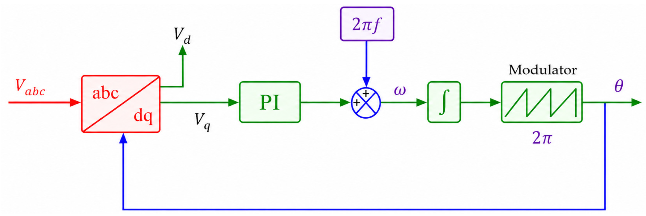
The PLL is defined as a phase-tracking method providing the frequency and phase information that are synchronized with its reference inputs. The aim of this method is to synchronize the output current of the inverter with the grid voltage, ensuring unity power factor. The block diagram of the PLL algorithm applied in the synchronous reference frame is shown in Figure 9 [4,24].

Inputs to the PLL are three phases of voltage taken from the grid-side measurements, while the output of the PLL refers to the tracking phase angle. In this respect, the PLL works within a dq synchronous reference frame, requiring a Park transform. To achieve phase synchronization, it should be ensured that there is no voltage on the q-axis. Generally, a PI controller is used for this task, and integration of the output of this controller with the reference frequency gives the desired phase angle [24,56].

11.2. Inner Current Controller

This presented inner current control loop is the core of the VSC control scheme; it tracks the current references ($i_d^{*}$ and $i_q^{*}$) generated via the outer loop and generates the final voltage references ($v_d^{*}$ and $v_q^{*}$) sent to the PWM generator. Also, ensures the converter currents stay within desired limits. The dynamic behavior that results from the converter’s phase reactor is described by applying Kirchhoff’s voltage law directly to the AC side of the VSC; the voltage balance equations in the stationary frame are given by Equation (19) [13]:

$$v_c=L{\displaystyle \frac{di}{dt}}+Ri+u$$

(19)

where $u$ is the point of common coupling (PCC) voltage, $v_c$ is the voltage at the converter side, $R$ and $L$ are the resistance and reactance of the phase reactor, and $i$ is the current of the phase reactor.

The voltage balance equations in $dq$ frame are:

$$u_d-v_{d,c}=R{i}_d+L{\displaystyle \frac{d{i}_d}{dt}}-\mathsf{\omega }L{i}_q$$

(20)

$$u_q-v_{q,c}=R{i}_q+L{\displaystyle \frac{d{i}_q}{dt}}+\omega L{i}_d$$

(21)

To achieve independent control of $i_d$ and $i_q$, feed-forward decoupling terms are used. Utilizing (PI) controllers, the control laws that generate the converter modulating voltage references ($v_d^{*}$ and $v_q^{*}$) are formulated as:

$$v_d^{\ast }=u_d-\left(K_p+{\displaystyle \frac{K_i}{s}}\right)\left(i_d^{\ast }-i_d\right)+\omega L{i}_q$$

(22)

$$v_q^{\ast }=u_q-\left(K_p+{\displaystyle \frac{K_i}{s}}\right)\left(i_q^{\ast }-i_q\right)-\omega L{i}_d$$

(23)

where ($u_d$, $u_q$): grid feedforward voltage and the cross-coupling cancellation ($\mathsf{\omega }L{i}_q,\mathsf{\omega }L{i}_d$) created by the phase reactor between the $d$ and $q$ axes.

By using ($v_d^{*}$ and $v_q^{*}$) formulas, we obtained a block diagram of the inner current controller structure in the $dq$ frame as in Refs. [24,25].

11.3. Outer Loop Controllers

The outer control loop consists of a DC voltage controller, an AC voltage controller, an active power controller, a reactive power controller, and a frequency controller, which regulate the corresponding quantity according to a reference value via generating reference currents ($i_d^{*}$ and $i_q^{*}$) which feed into the inner current controller.

11.3.1. DC Voltage Controller

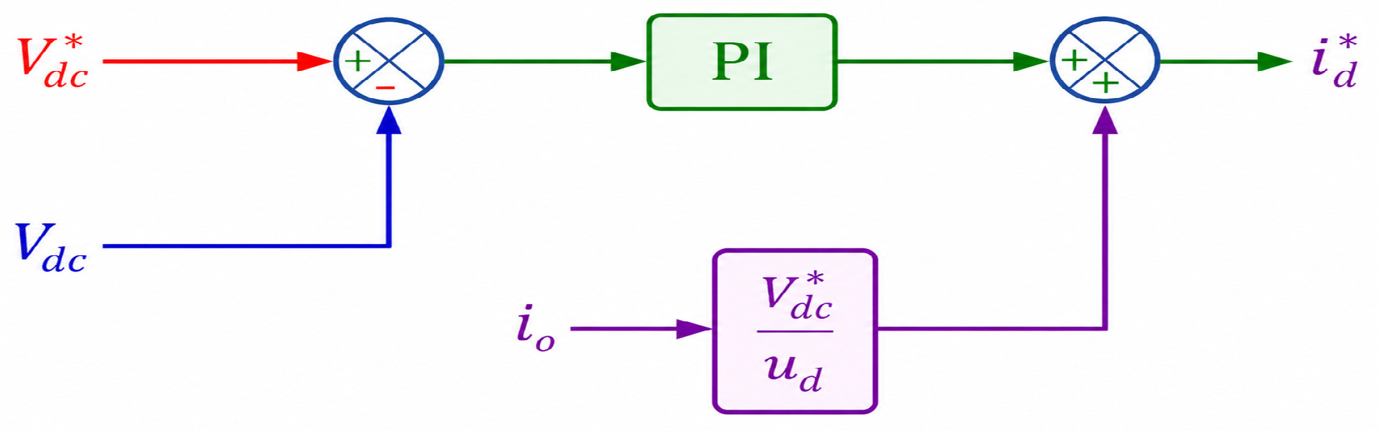
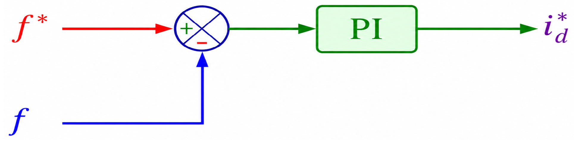
The DC voltage controller controls the DC link voltage to its reference value. The active current reference ($i_d^{*}$) is the output of the DC voltage controller. Figure 10 shows the block diagram of the DC voltage controller [22,24].

11.3.2. Active Power Controller

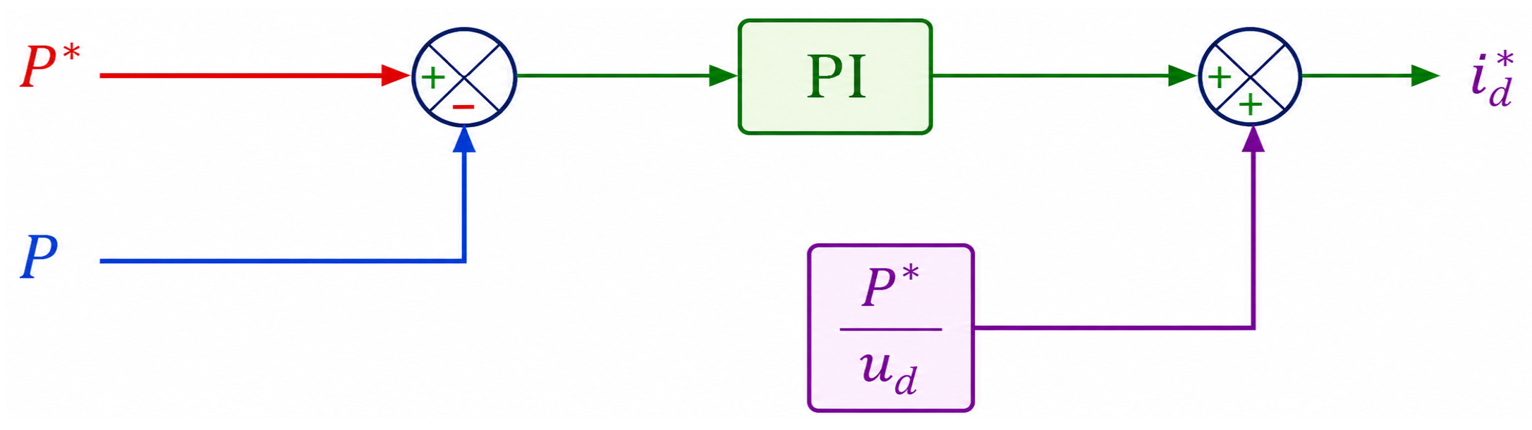
For simplicity, the active power controller is considered a standard proportional controller. The reference value of active current ($i_d^{*}$) is found through instantaneous power relations; the instantaneous active and reactive powers are expressed in Equations (24) and (25) [22,24]:

$$P=u_d{i}_d+u_q{i}_q$$

(24)

$$Q=u_q{i}_d-u_d{i}_q$$

(25)

Using the above relations along with decoupling of active and reactive currents, the active current reference is computed as follows:

$$i_d^{\ast }={\displaystyle \frac{P^{\ast }{u}_d-Q^{\ast }{u}_q}{u_d^2+u_q^2}}$$

(26)

where $P^{*}$ and $Q^{*}$ are active and reactive power references, $u_{d },u_q$ represent the dq-axis voltages of the grid and $i_d^{*}$ is the active current reference value.

The block diagram of the active power controller is shown in Figure 11.

11.3.3. Reactive Power Controller

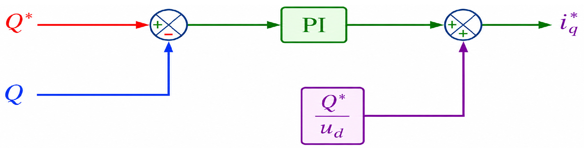
Analogous to the active power controller, the reactive power controller calculates the required value of the reactive current reference ($i_q^{*}$) according to the desired reactive power injection or absorption. The reactive current reference ($i_q^{*}$) is calculated from Equations (24) and (25) of instantaneous power [22,24]:

$$i_q^{*}={\displaystyle \frac{P^{*}{u}_q+Q^{*}{u}_d}{u_d^2+u_q^2}}$$

(27)

Figure 12 shows the block diagram of the reactive power controller:

11.3.4. AC Voltage Controller

AC voltage controller regulates the magnitude of the AC voltage at the point of common coupling (PCC) to its reference value. For the robust operation of a stable AC power grid, PQ control is advised. However, in some cases, especially in weak AC power grids, the need for PCC voltage regulation arises. In this case, the converter regulates the voltage by changing the current corresponding to reactive power, not controlling the reactive power itself. According to the literature, there are two methods for controlling AC voltage [22,57].

(a)

First Strategy:

The first method provides control of AC voltage by changing the voltage drop across the phase reactor of the Voltage Source Converter (VSC), shown in Figure 4. The voltage drop $\Delta \mathrm{V}$ at the reactor ${\mathrm{X}}_v$ is calculated according to the following formula [24]:

$$\begin{array}{c}\Delta V={\mathrm{V}}_{2\mathrm{i}}-{\mathrm{V}}_{1\mathrm{i}} =\Delta {\mathrm{V}}_{\mathrm{p}}+j\Delta {\mathrm{V}}_{\mathrm{q}} \\ \\ ={\displaystyle \frac{{\mathrm{R}}_v\mathrm{P}+{\mathrm{X}}_v\mathrm{Q}}{{\mathrm{V}}_{1\mathrm{i}}}}+j{\displaystyle \frac{{\mathrm{X}}_v\mathrm{P}-{\mathrm{R}}_v\mathrm{Q}}{{\mathrm{V}}_{1\mathrm{i}}}}\end{array}$$

(28)

If $\Delta {\mathrm{V}}_{\mathrm{q}}\ll {\mathrm{V}}_{1\mathrm{i}}+\Delta {\mathrm{V}}_{\mathrm{p}}$, then the voltage drop is expressed through its real component as:

$$\Delta \mathrm{V}\approx {\displaystyle \frac{{\mathrm{R}}_v\mathrm{P}+{\mathrm{X}}_v\mathrm{Q}}{{\mathrm{V}}_{1\mathrm{i}}}}$$

(29)

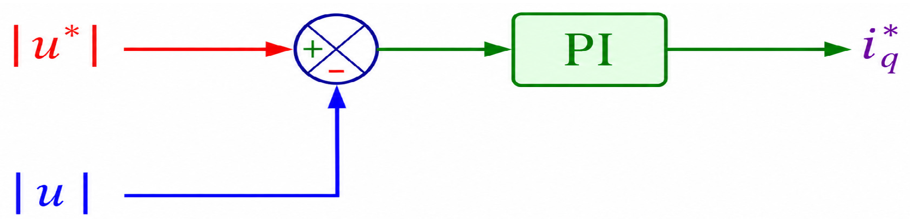
In typical AC power circuit operations, inductive reactance is significantly greater than the resistance (${\mathrm{X}}_v\gg {\mathrm{R}}_v$). Consequently, the voltage drop $\Delta \mathrm{V}$ becomes primarily dependent only upon the flow of reactive power ($\mathrm{Q}$). As a result, the variation in AC voltage ${\mathrm{V}}_{1\mathrm{i}}$ is determined exclusively by the reactive power flowing through the system. Equations (25) and (29) produce the block diagram of the AC voltage controller as shown in Figure 13 [22,57] where $\left|u\right|$ and $\left|u^{*}\right|$ are the amplitude and reference value of the line voltage.

(b)

Second Method:

For the second method, AC voltage control is performed through controlling the voltage droop across the AC filter capacitor ($C_f$). For the second method, AC voltage control is performed through controlling the voltage droop across the AC filter capacitor ($C_f$), just as in the case of the current inner control loop. The proposed AC voltage controller is designed in the dq frame as in Refs. [6,58].

Also consider the following disadvantage when applying the control algorithm in the dq-frame: it requires converting the measured AC voltages and currents into dq quantities with the help of a Phase-Locked Loop (PLL) that ensures synchronization between the converter voltage and the line voltage. As a consequence, the performance of the proposed control scheme heavily relies on the performance of the PLL control [22].

11.3.5. Frequency Controller

The main function of the frequency controller is to maintain the system frequency at its reference value. The network stiffness is characterized as the difference in power with respect to a unit change in the frequency in a linked AC system. The power versus frequency curve is depicted in a linear manner according to Equation (30):

$${\displaystyle \frac{\Delta P}{\Delta f}} = K$$

(30)

where $\Delta P$ is the power unbalance (difference between generation and demand), $\Delta f$ is the frequency drift or deviation from the reference, and $K$ is the system stiffness constant. A large $K$ means the system is “stiff,” and the frequency will not move much even with large power swings.

So, according to Equations (24) and (30), it can be said that implementation of a PI controller in the feedback circuit of the frequency will be sufficient. Figure 14 shows the block diagram of the frequency controller [25].

It must be emphasized that the function of the frequency controller is to provide power supply to the system in the absence of any other means of controlling frequency in the system. However, if there are two or more sources for controlling the frequency in a system, then a proportional controller must be utilized to distribute the load fluctuations over the sources [22,37].

12. Advantages of VSC-HVDC Systems

VSC-HVDC is preferred because of the following properties [3,22,32]:

•

The converter separately regulates active and reactive powers.

•

Capability to produce ideal sinusoidal voltage waveforms, decreasing the need for filtering.

•

The converter is capable of producing a lagging or leading phase angle of the voltage for rapid control of its active power, which improves the frequency stability without increasing cost.

•

It can provide power to highly weak AC networks and passive loads, and it has a black start ability.

•

Improved AC fault ride-through capabilities.

•

The converter can instantly respond with power inversion without changing the polarity of the DC voltage.

•

There is no need for rapid communication between the converter stations, as reactive and active power are controlled independently.

•

Reactive power regulation is independent of other terminals.

•

No need for communication between stations during normal operation.

•

A simpler link with the AC system.

•

The conversion process for DC transmission does not require transformers if its voltage matches the AC voltage. VSCs can control active and reactive power separately; therefore, they do not rely on transformer tap changers to maintain power factor. LLC requires transformers for phase shifting and to cancel harmonics.

•

Continuous AC voltage regulation.

•

There are no minimum power limitations.

•

No possibility for commutation failures.

•

There are no limitations on many different links.

•

Adjustable frequency capability.

13. Optimal Controller Design Based on Evolutionary Techniques

13.1. Advanced Controller Topologies Applied to VSC-HVDC Systems

13.1.1. Proportional–Integral Controller (PI)

Reason: PI controllers were widely utilized in various industrial control systems owing to their simple construction, reliable performance, and low cost [59].

Concept: A PI controller, as demonstrated in Figure 15, is a feedback control loop mechanism that uses two terms, proportional control and integral control, to continuously adjust a system to a desired setpoint. Proportional control aims to minimize rise and settling times, while integral control seeks to eliminate the steady-state error in the system [60].

Disadvantages: These controllers provide greater performance only within a limited operating range and must be adjusted if the operating range changes. Furthermore, PI controllers’ performance does not meet predictions for nonlinear and complex systems [61].

13.1.2. Variable Coefficient PI Controller (V-PI)

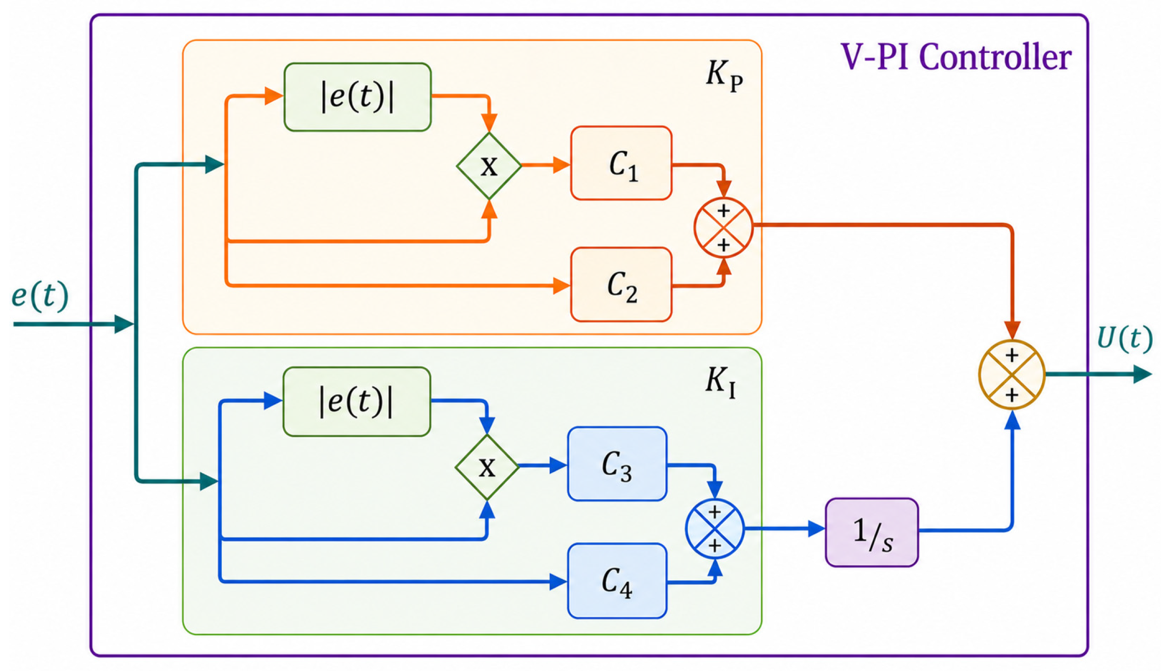
Reason: The traditional PI controller is characterized by fixed gains such as the proportional gain ${\mathrm{K}}_{\mathrm{P}}$ and integral gain ${\mathrm{K}}_{\mathrm{I}}$. These two gains are fixed and remain unchanged regardless of changes in error in the system, so the same structure must handle both large transient errors and small steady-state errors, which can lead to a compromise in performance. As a result, it is difficult, with the use of constant parameters, to enhance the transient and steady-state responses independently [62].

Concept: The Variable Coefficient PI controller, Figure 16, identified as a Nonlinear PI controller, is differentiated by its varying coefficient gains symbolized by ${\mathrm{K}}_{\mathrm{P}}^{\prime }$ and ${\mathrm{K}}_{\mathrm{I}}^{\prime }$, the values of (${\mathrm{K}}_{\mathrm{P}}^{\prime }$ and ${\mathrm{K}}_{\mathrm{I}}^{\prime }$) gains will change depending on the error of the system, and therefore the variable coefficients improve transient response and steady-state performance separately. The variable coefficients are defined as ${\mathrm{K}}_{\mathrm{P}}^{\prime }={\mathrm{c}}_1\left|\mathrm{e}\left(\mathrm{t}\right)\right|+{\mathrm{c}}_2$ and ${\mathrm{K}}_{\mathrm{I}}^{\prime }={\mathrm{c}}_3\left|\mathrm{e}\left(\mathrm{t}\right)\right|+{\mathrm{c}}_4$, where $\left|e\left(t\right)\right|$ is the system’s absolute error, also ${\mathrm{c}}_1$ through ${\mathrm{c}}_4$ are the tuning parameters of the variable coefficient gains [63].

Figure 16. Variable Coefficient PI Controller (V-PI).

Figure 16. Variable Coefficient PI Controller (V-PI).

Advantages: This unique V-PI approach allows for improving the responses of the control system under both transient and steady-state conditions individually. Moreover, along with offering increased flexibility when designing PI controllers, the new approach provides an opportunity to precisely control the system dynamics [62].

13.1.3. Fuzzy PI Controller (F-PI)

Reason: Fuzzy PI controllers can effectively control complex nonlinear systems and can deal with systems with varying operating conditions.

Concept: The Fuzzy PI, displayed in Figure 17, is a control system that combines the logic of a conventional PI controller with the decision-making of fuzzy logic. Instead of using fixed proportional and integral gains, it uses a fuzzy inference system with rules based on the error along with its rate of change to determine the control output [64].

Advantages: Fuzzy PI controllers handle uncertainty and adapt their behavior, providing more diversity and often better performance in nonlinear or complex systems compared to a standard PI controller [64].

Disadvantages: The performance is significantly dependent on the quality of the fuzzy rules, which requires significant expert knowledge, in addition to computational complexity problems, the absence of systematic design, and lack of learning and training abilities [65].

13.1.4. Self-Tuning Fuzzy PI Controller (STF-PI)

Reason: The PI controller performance depends upon the precision of system models and parameters. As a result, many researchers today are interested in applying intelligent control techniques that could deal with uncertain dynamics and nonlinearity within the system and achieve the desired response [65].

Concept: The STF-PI controller, demonstrated in Figure 18, combines the PI controller with the fuzzy logic control strategy and can perform automatic tuning of the PI controller parameters online. FLC transforms a classical PI controller into an adaptive controller. In the suggested strategy, the ‘Mamdani-type’ FLC structure employs the error (e) and its rate of change (de/dt) as inputs to compute two outputs ${\mathrm{K}}_{\mathrm{P}}$ and ${\mathrm{K}}_{\mathrm{I}}$ [66].

Advantages: The input and output parameters have quite a nonlinear relationship; the values of the proportional and integral gains vary with increasing error amplitude and rate of change in error, and vice versa [67].

13.1.5. Fractional Order PI Controller (FOPI)

Reason: Conventional integer-order PI controller sometimes struggles to achieve a good balance between transient response, steady-state accuracy, and robustness, especially for systems with time delays, high-order dynamics, or fractional order behavior. The FOPI controller is introduced to overcome these limitations by generalizing the integral action (${\mathrm{K}}_{\mathrm{I}}$) from integer-order to fractional order ($\lambda$), which gives extra tuning flexibility [61].

Concept: Compared with the PI controller, the FOPI controller displayed in Figure 19 is distinguished by an extra control parameter, which is the fractional order (λ) of the integral part. Including fractional calculus in a PI controller gives greater flexibility in controller design and improves dynamic performance. Parameter $\lambda$ primarily impacts the integral links of the controller, and its range is adjusted based on the order of the system. The fractional order ($\lambda$) mainly influences the system’s steady accuracy, adjustment time, and robustness [68].

Advantages of FOPI Controller [61]:

(i).

Better Performance Metrics: FOPI controllers outperform traditional PID controllers in terms of the rise time, the settling time, the overshoot, and the steady-state errors, especially for nonlinear, delayed, or high-order systems.

(ii).

Enhanced Robustness and Disturbance Rejection: The inclusion of extra degrees of freedom (fractional orders) gives FOPI greater flexibility and robustness to plant uncertainties, parameter variation, and external disturbances, while enhancing the control system’s robustness, accuracy, dynamics, and stability.

(iii).

Flexibility For Complex Systems: FOPI is mainly effective for fractional order systems (e.g., power-system models) where the controller order naturally “matches” the system dynamics, leading to smoother control signals and improved stability.

13.1.6. Variable Coefficient Fractional Order PI Controller (V-FOPI)

Reason: Compared to Classical FOPI, the V-FOPI controller is distinguished by an extra control parameter, which is the fractional order (λ) of the integral terms, which improves robustness and performance for many nonlinear systems. However, its gains and fractional orders are fixed, so the same structure must handle both large transient errors and small steady-state errors, which can lead to a reduction in performance [63].

Concept: The Variable Coefficient Fractional Order PI controller, shown in Figure 20, is differentiated by its variable coefficient gains symbolized by ${\mathrm{K}}_{\mathrm{P}}^{\prime }$ and ${\mathrm{K}}_{\mathrm{I}}^{\prime }$. These gains have been established by the current error values. Consequently, the values of (${\mathrm{K}}_{\mathrm{P}}^{\prime }$ and ${\mathrm{K}}_{\mathrm{I}}^{\prime }$) gains alter as a function of system error; also, these variable coefficients manage to improve the transient and steady-state responses independently. These variable coefficients are defined as $K_P^{\prime }=c_1\left|e\left(t\right)\right|+c_2$ and $K_I^{\prime }=c_3\left|e\left(t\right)\right|+c_4$, where $\left|e\left(t\right)\right|$ is the system’s absolute error, and ($c_1$ to $c_4$) are tuning parameters of variable coefficients. In addition, tuning the integral fractional order ($\lambda$) mostly influences the system’s steady accuracy and adjustment time [62].

Advantages of V-FOPI Controller [69]:

•

Enhanced Transient and Steady-State Performance: By utilizing variable gains, the V-FOPI can separately optimize speed of response and overshoot/oscillation suppression, outperforming PID, V-PID, and fixed-coefficient controllers. FOPI permits improving system responses in both transient and steady-state conditions separately.

•

Greater Robustness and Design Flexibility: The fractional orders and variable coefficients add extra tuning flexibility, allowing for superior disturbance rejection, tracking, and robustness to parameter variations.

•

Better Handling of Nonlinear and Uncertain Systems: The combination of fractional order dynamics and variable gains makes the V-FOPID highly suitable for nonlinear, time-delayed, or uncertain systems where fixed-gain controllers struggle to keep reliable performance across operating points.

13.1.7. Adaptive Neuro-Fuzzy Inference System (ANFIS) Controller

Definition: The Adaptive Neuro-Fuzzy Inference System (ANFIS) controller is defined as a hybrid intelligent controller that combines the learning capability of the artificial neural network (ANN) with the reasoning and linguistic capabilities of a fuzzy inference system (FIS) [70].

Reason: The ANFIS controller is capable of learning complex and nonlinear input-output relationships directly from data, making it highly effective at modeling and controlling systems with complex nonlinear dynamics.

Concept: The ANFIS controller utilizes the Takagi–Sugeno fuzzy model that uses a five-layer network architecture. The controller’s development involves an offline training phase using a dataset that contains input-output pairs of the desired system behavior. The training process uses a hybrid learning algorithm to optimize the controller’s parameters [71].

Advantages of ANFIS Controller [72]:

(i).

Superior Performance: ANFIS controller achieves superior performance for nonlinear systems where conventional control methods often perform poorly.

(ii).

Adaptability and Robustness: The controller’s built-in learning mechanism enables it to respond to various system conditions and external disturbances in real time.

(iii).

Automatic Rule Generation: Unlike typical fuzzy logic controllers, which require manual adjustment of rules and membership functions, ANFIS can learn and optimize these parameters using input-output training data.

(iv).

High Accuracy: ANFIS can achieve higher accuracy and faster response times compared to a standard fuzzy logic controller.

(v).

Model-Free Control: It does not need a precise mathematical model of the system, but rather relies on data-driven training. This is a significant advantage for complex systems where accurate mathematical modeling is difficult.

13.1.8. Model Predictive Controller (MPC)

Definition: Model Predictive Control (MPC) is a more advanced control approach that employs a dynamic model for predicting a system’s future behavior over a finite time horizon. The controller then computes a sequence of optimal control actions to drive the system toward a desired state while satisfying operational constraints [73].

Working Concept: The Model Predictive Control algorithm operates in a continuous loop and involves three main components [74]:

• Predictive Model: An internal mathematical model of the process is utilized to estimate the system’s future output trajectory across a specified time period, known as the prediction horizon. The model utilizes current and past system measurements and a sequence of future control inputs.
• Cost Function: An objective function is minimized to find the optimal control inputs. This objective function typically ignores deviations from the desired reference trajectory and minimizes control action to ensure a smooth and efficient response.
• Optimization: At each time step, an optimization algorithm determines the sequence of future control actions that will minimize the cost function. It accomplishes this while taking into consideration hard constraints such as physical limitations on actuators and soft constraints.

Advantages of Model Predictive Controller [74]:

(a)

Optimal Constraint Handling: MPC is mainly effective at handling system constraints in a systematic and optimal way.

(b)

Multivariable Control: It naturally handles multiple interacting inputs and outputs (MIMO systems), coordinating them to produce higher performance over multiple single-loop controllers.

(c)

Disturbance Rejection: The controller’s receding horizon and predictive nature allow it to predict and respond to future disturbances, leading to more robust control.

(d)

Handling Complex Systems: It can control complex, nonlinear, and unstable open-loop systems without requiring complex modifications.

(e)

Enhanced Performance: MPC is able to increase operational efficiency and safety by allowing the system to operate closer to its performance boundaries.

13.2. Optimal Design Based on Optimization Techniques

There have been several evolutionary methods suggested in the existing literature that can be used for obtaining the optimal PID controller parameters in a variety of applications. In this report, it is suggested to utilize Particle Swarm Optimization (PSO), Phasor Particle Swarm Optimization (PPSO), Gravitational Search Algorithm with Particle Swarm Optimization (GSA-PSO), and Eagle Strategy with Particle Swarm Optimization (ES-PSO) for optimal tuning of several controllers proposed for VSC-HVDC.

13.2.1. Objective Function Formulation

One of the key elements in designing optimal controllers is choosing an appropriate objective function. In this study, the Integral of Time Absolute Error (ITAE) objective function $\left(J_1\right)$ given by Equation (31), and the dynamic performance indices objective function ${(J}_2$) given by Equation (32) will be used for the optimal controller design [75].

$$J_1=\mathrm{I}\mathrm{T}\mathrm{A}\mathrm{E}={\int }_0^{\infty }t\left|e\left(t\right)\right|dt$$

(31)

$$J_2={\int }_0^{\mathrm{\infty }}{\delta }_1\left|e\left(t\right)\right|dt+{\delta }_2\ast OS\%+{\delta }_3\ast {(t}_s-t_r)$$

(32)

$e\left(t\right)$ is the time-domain error signal, $OS\%$ represent the overshoot percentage, $t_r$ and $t_s$ are the rise and settling times, respectively, and finally ${\delta }_1,{\delta }_2 and {\delta }_3$ are defined as weighting factors utilized to adjust the significance of different performance criteria.

13.2.2. Particle Swarm Optimization

Particle Swarm Optimization (PSO) is an entirely novel meta-heuristic population-dependent stochastic optimization approach. It uses evolutionary search to find solutions that are near-optimal or optimal. During each iteration, each particle adjusts its position ($\mathrm{X}$) depending on its own experience ($Pbest$) and the experience of particles in its global neighborhoods ($Gbest$). Every particle in a PSO swarm is connected to or may interact with every other particle in the swarm. Equations (33) and (34) are used to update the velocity and location of particles [76].

$$V_i^{\left(Iter+1\right)}=\omega V_i^{Iter}+C_1{r}_1\left({Pbest}_i^{Iter}-X_i^{Iter}\right)+C_2{r}_2\left({Gbest}_i^{Iter}-X_i^{Iter}\right)$$

(33)

$$X_i^{(Iter+1)}=X_i^{\left(Iter\right)}+V_i^{(Iter+1)}$$

(34)

Working Steps of PSO Technique

The PSO can be summarized in the following phases [69]:

• Step 1. Load Parameters of the System.
• Step 2. Initial Population Generation.
• Step 3. Update Best Fitness at Current Iteration.
• Step 4. Update Particle Velocity and Update Its Position.
• Step 5. Examine Stopping Criterion.
• If  yes  move to Step 6.
• else     move to Step 3.
• Step 6. Outputs Optimal Solution.

13.2.3. Phasor Particle Swarm Optimization (PPSO)

Phasor Particle Swarm Optimization (PPSO) is a novel and straightforward adaptive model developed to overcome the increasing complexity and limitations of real-life, high-dimensional problems that traditional adaptive PSO algorithms struggle to optimize efficiently. Inspired by mathematical phasor theory, PPSO models particle control parameters by transforming them into functions of a phase angle ($\theta$), converting the algorithm into a self-adaptive, trigonometric, balanced, and nonparametric meta-heuristic method with simpler computations. To achieve this, every particle ($i$) is defined through a one-dimensional phase angle (${\theta }_i$), allowing each particle to be represented by a magnitude vector as $\overrightarrow{X_i}=\left|X_i\right|\angle {\theta }_i$. As the phase angle naturally oscillates, it dynamically regulates the search behavior, allowing PPSO to inherently sustain a critical balance between broad global search and focused local search. Consequently, this trigonometric-based adaptation not only streamlines the algorithm’s computation but also effectively prevents the swarm from prematurely converging on local optima, ensuring a more reliable and efficient search for the global best solution by dynamically speeding up or slowing down the rise of $Pbest\left({\theta }_i^{iter}\right)$ and $Gbest\left({\theta }_i^{iter}\right)$ in either the same or opposite directions. Subsequently, Equations (35) and (36) are applied to modify the velocity and position of each particle during every iteration [69,77].

$$\begin{array}{cc}\hfill {\overrightarrow{V }}_i^{Iter+1}& =\left({\left|\cos |\left({\theta }_i^{Iter}\right)\right|}^{2\sin \left({\theta }_i^{Iter}\right)}|/|N\right)V_i^{Iter}+{\left|\cos |\left({\theta }_i^{Iter}\right)\right|}^{2\sin \left({\theta }_i^{Iter}\right)}\hfill \\ & \ast \left({Pbest}_i^{Iter}-X_i^{Iter}\right){+\left|\sin |\left({\theta }_i^{Iter}\right)\right|}^{2\cos \left({\theta }_i^{Iter}\right)} \left({Gbest}_i^{Iter}-X_i^{Iter}\right)\hfill \end{array}$$

(35)

Equation (36), on the other hand, updates the particle position as follows:

$${ \overrightarrow{X }}_i^{Iter+1}={ \overrightarrow{ X }}_i^{Iter}+{ \overrightarrow{ V }}_i^{Iter+1}$$

(36)

The PPSO algorithm flow chart, which summarizes the method’s working phases in detail, is depicted in Ref. [69].

13.2.4. Gravitational Search Algorithm with PSO

The Gravitational Search Algorithm with PSO (GSA-PSO) is a combination of Particle Swarm Optimization (PSO) plus Gravitational Search Algorithm (GSA). The core concept of GSA-PSO is to integrate PSO’s global search ($\mathrm{G}\mathrm{b}\mathrm{e}\mathrm{s}\mathrm{t}$) ability along with GSA’s local search ability. Agents close to the ideal solution attempt to attract other agents that explore the search region. When all agents are extremely close to the optimal solution, they begin moving incredibly slowly [78]. In this case, the PSO’s $Gbest$ significantly assists them in exploring the global search space. GSA-PSO stores the best solution identified thus far in memory $\mathrm{G}\mathrm{b}\mathrm{e}\mathrm{s}\mathrm{t}$ to make it available to all agents. The capabilities of global and local searches are controlled by adjusting the weighting factors ($C_1^{\prime } \mathrm{a}\mathrm{n}\mathrm{d} C_2^{\prime }$) [63,78].

Working Steps of GSA-PSO Techniques

The GSA-PSO is composed of the following steps as outlined below [63]:

• Step 1. Loading Parameters of the System.

Load the fitness function, variables, and the system’s constraints.

• Step 2. Initial Population Generation.

Agents are produced randomly; each agent is considered a possible solution.

• Step 3. Compute the Fitness of Each Agent and Update the Best Fitness at the Current Iteration.
• Step 4. Update the Parameters of the GSA-PSO Algorithm.

Once the iteration is completed, update the gravitational constant, best and worst fitness, and inertia mass.

• Step 5. Compute Gravitational Force and Total Force.

$F_{ij}^{Iter}$ is the gravitational force that is applied to agent i from another agent j.

$F_i^{Iter}$ is the total force that is applied to agent i from all agents, computed by Equation (37):

$$F_i^{\left(Iter\right)}={\displaystyle \sum _{j=1,j\ne i}^N}{rand}_j{F}_{ij}^{\left(Iter\right)}$$

(37)

• Step 6. Compute the Acceleration of Agents (${ac}_i^{\left(Iter\right)}$).

  $${ac}_i^{\left(Iter\right)}={\displaystyle \frac{F_i^{\left(Iter\right)}}{M_{ii}^{\left(Iter\right)}}}$$

  (38)

  $M_{ii}$ is the inertial mass of agent i.

• Step 7. Compute Agent Velocity and Update Its Position.

The next velocity of every agent gets modified using Equation (39):

$$V_i^{\left(Iter+1\right)}=\omega \ast V_i^{\left(Iter\right)}+{C_1^{\prime }\ast r_1\ast ac}_i^{\left(Iter\right)}+C_2^{\prime }{r}_2\left({Gbest}_i^{\left(Iter\right)}-X_i^{\left(Iter\right)}\right)$$

(39)

where $\omega$ is a weighting function and $C_1^{\prime },C_2^{\prime }$ are a weighting factor.

Equation (40) is used to upgrades each agent’s next position:

$$X_i^{(Iter+1)}=X_i^{\left(Iter\right)}+V_i^{(Iter+1)}$$

(40)

• Step 8. Examine Stopping Criterion.
• If   (Iter = Max Iteration), move to Step 9.
• else,   move to Step 3.
• Step 9. Output Optimum Solution.

Finally, if the GSA-PSO algorithm meets an end criterion, it will be terminated, and the most effective agents will be printed.

The flowchart of the GSA-PSO methodology, which summarizes the strategy steps, is represented in Ref. [63].

13.2.5. Eagle Strategy with Particle Swarm Optimization

Eagle Strategy with Particle Swarm Optimization (ES-PSO) is defined as a meta-heuristic technique that iteratively searches for the best solution. ES-PSO is a two-stage technique made up of a global search stage as well as a local search stage. At the start, ES-PSO uses Lévy flight walks to explore the search space globally; once a possible solution has been identified, it moves to the local search phase to execute an intensive local search using the PSO algorithm. These two phases continue iterating until one of the stopping criteria is fulfilled. In fact, numerous algorithms can be combined during the global optimization stage and local optimization stage. ES-PSO employs the advantages of these different algorithms to generate improved results [63,79].

Working Steps of ES-PSO Strategy

The teps of the proposed ES-PSO method have been explained as follows [63]:

• Step 1. Load Parameters of the System.

Load the fitness function, variables, and system constraints.

• Step 2. Random Creation of the Initial Population.

Random creation of particles is carried out, where each particle is considered a feasible solution.

• Step 3. Global Search Stage and Update Best Fitness.

Random global search is performed using Lévy flight. Once a good solution has been found, move to Step 4.

• Step 4. Switching Between Global and Local Search Stages.

The switching probability p determines the alternation of global and local searches.

•    If  $p<rand$  move to the local search step (Step 5)
•    else    move to the global search step (Step 7)
• Step 5. Intensive Local Search Stage.

Execute a highly intensive local search for the optimum solution.

Update each particle’s velocity and position as follows.

$$V_i^{Iter+1}={\mathsf{\alpha }}^{Iter}{*V}_i^{Iter}+C_1{r}_1\left({Pbest}_i^{Iter}-X_i^{Iter}\right) {+C}_2{r}_2\left({Gbest}_i^{Iter}-X_i^{Iter}\right)$$

(41)

$$\mathrm{where} {\mathsf{\alpha }}^{\left(Iter\right)}={\mathsf{\alpha }}_{max}*{\displaystyle \frac{Iter({\mathsf{\alpha }}_{max}-{\mathsf{\alpha }}_{min})}{MaxIter}}$$

(42)

The particle position is updated via Equation (43).

$$X_i^{(Iter+1)}=X_i^{\left(Iter\right)}+V_i^{(Iter+1)}$$

(43)

Then, update the best solution in the local search stage.

• Step 6. Update Global Best Fitness and Global Best Position in the Overall Strategy.

The global best fitness and global best position in the ES-PSO strategy are updated.

Finally, update the optimal solution for the overall ES-PSO strategy:

• Step 7. Update Iteration (Iter = Iter + 1).
• Step 8. Examine Stopping Criterion.
•    If  (Iter = Max Iteration), move to Step 9.
•    else,  move to Step 3.
• Step 9. Output Best Solution.

Finally, if (ES-PSO) meets an end criterion, it will be terminated, and the most effective particles will be printed.

The flowchart of the ES-PSO methodology, which summarizes the strategy steps, is represented in Ref. [63].

14. Comprehensive Analysis of VSC Control Strategies in Machine Drives and HVDC Transmission Systems

The assessment of each literature considered the methodology employed, the performance claims made by the authors, the reported performance metrics, and a critical review of the advantages in addition to limitations. The assessment therefore does not rely on a single performance indicator or on the authors’ personal preference. Table 5 demonstrates a comprehensive analysis of advanced control strategies for Voltage Source Converters fed machine-drive systems and VSC-HVDC transmission systems.

Table 5. Comprehensive analysis of VSC control strategies.

Authors & Year	Paper Title	Methodology	Claims by Author	Performance Metrics	Advantages	Limitations
[80] Sime et al. (2024)	Modeling of genetic algorithm tuned adaptive fuzzy fractional order PID speed control of permanent magnet synchronous motor for electric vehicle	The study develops a PMSM model within an electric vehicle dynamics framework and designs a hybrid controller merging fractional order PID with adaptive fuzzy logic. A genetic algorithm automatically tunes the (GA-AFFOPID) controller’s parameters for PMSM speed regulation in MATLAB/Simulink.	The controller achieves precise speed tracking with minimal overshoot and settling time, demonstrating strong robustness against parameter variations and load disturbances while significantly outperforming classical PID and FOPID controllers	The controller’s efficacy is evaluated using time-domain specifications, specifically overshoot percentage, settling time, rise time, and steady-state error.	Offers automatic parameter tuning, high tracking precision, and strong handling of nonlinearities without complex math models.	The proposed controller faces potential challenges regarding computational complexity for real-time hardware use and currently lacks physical experimental validation.
[81] Mencou et al. (2025)	Advanced control of induction motors (2019–2025): A comprehensive review of strategies, algorithms and sensorless techniques	The authors systematically reviewed over 240 recent publications to categorize and critically analyze induction motor control advancements. The review comprehensively covers fundamental strategies, advanced algorithms, and sensorless techniques	The analysis reveals that AI-enhanced Direct Torque Control provides an optimal balance between torque dynamics and system robustness. Furthermore, hybrid control approaches are highlighted as promising future innovation for industrial drives.	The evaluated control techniques are assessed using transient response indicators such as rise time, settling time, overshoot, and steady-state error. Additionally, performance is measured by analyzing torque and flux ripples, total harmonic distortion, and robustness against parameter variations.	Provides a highly structured, up-to-date synthesis of recent literature, effectively mapping the evolution from basic to complex hybrid control systems.	Lacks original experimental validation or novel algorithms; merely catalogs existing theoretical performance constraints and literature trends.
[82] Fatemigarakani et al. (2025)	A General Vector Control Scheme for Induction Motor Drives	A generalized motor model using conventional transformations was developed and integrated into classic vector control via variable PI controllers.	This scheme offers a universal control solution for healthy three-phase, single-phase, and faulted induction motors without requiring major structural changes, with lower computational complexity.	Performance is evaluated using rise time, torque ripple, and robustness under both no-load and load conditions.	Reduces structural complexity by using only two variable PI controllers and a conventional transformation matrix while maintaining a constant switching frequency.	Retains medium computational complexity compared to basic control methods and relies heavily on accurate motor parameter estimation.
[83] Bhayo et al. (2025)	High precision experimentally validated adaptive neuro fuzzy inference system controller for DC motor drive system	An ANFIS controller was trained using data from a well-tuned PI setup. It was then simulated and experimentally validated on a dSPACE DS1104 board for both speed and torque loops	Completely eliminates the inherent PI trade-off by removing speed overshoot without sacrificing response speed, while maintaining excellent adaptability through its learning capability.	The controller performance is evaluated using percentage overshoot and settling time, measured during both software simulations and hardware experiments.	The method achieves absolute zero overshoot and a drastically faster 0.18s settling time experimentally compared to the PI controller	The ANFIS controller demands higher computational power and memory. Furthermore, its effectiveness relies heavily on the quality of the training data, and the study lacks validation under varying load conditions.
[7] Rhonali et al. (2025)	A Comparative Review of Advanced Control Strategies for VSC-HVDC Transmission Systems	Surveys and categorizes VSC-HVDC control strategies into three tiers: (1) conventional PI/PID; (2) advanced nonlinear methods; and (3) intelligent methods. A case study directly compares a well-tuned PI cascade against a Lyapunov-based backstepping controller.	The nonlinear backstepping controller significantly outperforms conventional PID by overcoming its inherent limitations with nonlinear dynamics, achieving superior DC voltage regulation and near-instantaneous power tracking.	Performance is evaluated using standard time-domain error indices (ISE, ITSE, IAE, and ITAE) calculated for both DC-link voltage and active power tracking errors.	Effectively bridges a comprehensive literature review with quantitative simulation validation. The backstepping method guarantees global asymptotic stability while explicitly handling system nonlinearities to deliver faster transients and minimal overshoot.	The study relies entirely on software simulations without physical hardware validation. The simulation case study is restricted to a basic two-terminal topology and does not validate the advanced strategies on the complex multi-terminal systems emphasized in the review.
[84] Liu et al. (2025)	Cooperative modular multilevel converter control based on PSO optimized fuzzy-PI and hierarchical finite-state model predictive control	The study combines an outer-loop Fuzzy PI controller, tuned offline via Particle Swarm Optimization, with an inner-loop hierarchical finite-state Model Predictive Control that maintains accurate current tracking.	The authors claim this coordinated strategy eliminates empirical weight factor tuning and drastically reduces computational complexity while maintaining full voltage-level output and highly accurate reference tracking.	Performance is evaluated using settling time, overshoot, steady-state error, total harmonic distortion (THD), peak circulating current, and average switching frequency.	This approach delivers faster transient responses, lower steady-state errors, and a 46% reduction in switching frequency, while cutting computational load by 93% regardless of the submodule count.	The offline optimization limits adaptability to large or sustained operating changes, and the findings currently lack physical hardware validation.
[85] Saleem et al. (2025)	An Intelligent Frequency Control Scheme for Inverting Station in HVDC Transmission	A MATLAB/Simulink model of an HVDC transmission system was developed to evaluate ANFIS, ANN, and PSO-optimized PID controllers for regulating inverter station frequency under various load disturbances.	The ANN controller proved most effective, accurately maintaining a strict 50 Hz frequency with minimal deviation under varying load conditions. These intelligent methods outperform traditional techniques.	Performance was evaluated based on the system’s ability to maintain a 50 Hz setpoint, alongside a magnitude of frequency deviations, response time to load changes, and settling time during transient events.	Intelligent controllers provide faster transient responses than traditional methods, with ANN showing superior adaptability for automated grid integration	The research relies entirely on software simulations without physical hardware validation, and Intelligent controllers’ performance strictly depends on training data quality.
[1] Abo-Khalil et al. (2026)	HVDC Systems and renewable energy in a comparative study of technologies and applications	The researchers carried out a techno-economic assessment of HVAC and HVDC transmission systems with regard to important factors like power loss, electromagnetic compatibility, and overall costs. Also, benchmarked various HVDC converter topologies.	The results demonstrate that for distances exceeding 80 to 100 km, HVDC systems provide superior efficiency, lower lifetime costs, and enhanced grid stability.	Key evaluation parameters include transmission power losses per 100 km, maximum economic transmission distance, total installation cost per kilometer, and Short-Circuit Ratio tolerance for weak grids.	Offers highly specific, data-driven comparisons (e.g., exact loss percentages and cost per kilometer) that clearly define practical engineering limits	As a review, it lacks experimental validation and merely identifies advanced challenges like AI-based fault protection without providing concrete solutions.

Table 5. Comprehensive analysis of VSC control strategies.

Authors & Year	Paper Title	Methodology	Claims by Author	Performance Metrics	Advantages	Limitations
[80] Sime et al. (2024)	Modeling of genetic algorithm tuned adaptive fuzzy fractional order PID speed control of permanent magnet synchronous motor for electric vehicle	The study develops a PMSM model within an electric vehicle dynamics framework and designs a hybrid controller merging fractional order PID with adaptive fuzzy logic. A genetic algorithm automatically tunes the (GA-AFFOPID) controller’s parameters for PMSM speed regulation in MATLAB/Simulink.	The controller achieves precise speed tracking with minimal overshoot and settling time, demonstrating strong robustness against parameter variations and load disturbances while significantly outperforming classical PID and FOPID controllers	The controller’s efficacy is evaluated using time-domain specifications, specifically overshoot percentage, settling time, rise time, and steady-state error.	Offers automatic parameter tuning, high tracking precision, and strong handling of nonlinearities without complex math models.	The proposed controller faces potential challenges regarding computational complexity for real-time hardware use and currently lacks physical experimental validation.
[81] Mencou et al. (2025)	Advanced control of induction motors (2019–2025): A comprehensive review of strategies, algorithms and sensorless techniques	The authors systematically reviewed over 240 recent publications to categorize and critically analyze induction motor control advancements. The review comprehensively covers fundamental strategies, advanced algorithms, and sensorless techniques	The analysis reveals that AI-enhanced Direct Torque Control provides an optimal balance between torque dynamics and system robustness. Furthermore, hybrid control approaches are highlighted as promising future innovation for industrial drives.	The evaluated control techniques are assessed using transient response indicators such as rise time, settling time, overshoot, and steady-state error. Additionally, performance is measured by analyzing torque and flux ripples, total harmonic distortion, and robustness against parameter variations.	Provides a highly structured, up-to-date synthesis of recent literature, effectively mapping the evolution from basic to complex hybrid control systems.	Lacks original experimental validation or novel algorithms; merely catalogs existing theoretical performance constraints and literature trends.
[82] Fatemigarakani et al. (2025)	A General Vector Control Scheme for Induction Motor Drives	A generalized motor model using conventional transformations was developed and integrated into classic vector control via variable PI controllers.	This scheme offers a universal control solution for healthy three-phase, single-phase, and faulted induction motors without requiring major structural changes, with lower computational complexity.	Performance is evaluated using rise time, torque ripple, and robustness under both no-load and load conditions.	Reduces structural complexity by using only two variable PI controllers and a conventional transformation matrix while maintaining a constant switching frequency.	Retains medium computational complexity compared to basic control methods and relies heavily on accurate motor parameter estimation.
[83] Bhayo et al. (2025)	High precision experimentally validated adaptive neuro fuzzy inference system controller for DC motor drive system	An ANFIS controller was trained using data from a well-tuned PI setup. It was then simulated and experimentally validated on a dSPACE DS1104 board for both speed and torque loops	Completely eliminates the inherent PI trade-off by removing speed overshoot without sacrificing response speed, while maintaining excellent adaptability through its learning capability.	The controller performance is evaluated using percentage overshoot and settling time, measured during both software simulations and hardware experiments.	The method achieves absolute zero overshoot and a drastically faster 0.18s settling time experimentally compared to the PI controller	The ANFIS controller demands higher computational power and memory. Furthermore, its effectiveness relies heavily on the quality of the training data, and the study lacks validation under varying load conditions.
[7] Rhonali et al. (2025)	A Comparative Review of Advanced Control Strategies for VSC-HVDC Transmission Systems	Surveys and categorizes VSC-HVDC control strategies into three tiers: (1) conventional PI/PID; (2) advanced nonlinear methods; and (3) intelligent methods. A case study directly compares a well-tuned PI cascade against a Lyapunov-based backstepping controller.	The nonlinear backstepping controller significantly outperforms conventional PID by overcoming its inherent limitations with nonlinear dynamics, achieving superior DC voltage regulation and near-instantaneous power tracking.	Performance is evaluated using standard time-domain error indices (ISE, ITSE, IAE, and ITAE) calculated for both DC-link voltage and active power tracking errors.	Effectively bridges a comprehensive literature review with quantitative simulation validation. The backstepping method guarantees global asymptotic stability while explicitly handling system nonlinearities to deliver faster transients and minimal overshoot.	The study relies entirely on software simulations without physical hardware validation. The simulation case study is restricted to a basic two-terminal topology and does not validate the advanced strategies on the complex multi-terminal systems emphasized in the review.
[84] Liu et al. (2025)	Cooperative modular multilevel converter control based on PSO optimized fuzzy-PI and hierarchical finite-state model predictive control	The study combines an outer-loop Fuzzy PI controller, tuned offline via Particle Swarm Optimization, with an inner-loop hierarchical finite-state Model Predictive Control that maintains accurate current tracking.	The authors claim this coordinated strategy eliminates empirical weight factor tuning and drastically reduces computational complexity while maintaining full voltage-level output and highly accurate reference tracking.	Performance is evaluated using settling time, overshoot, steady-state error, total harmonic distortion (THD), peak circulating current, and average switching frequency.	This approach delivers faster transient responses, lower steady-state errors, and a 46% reduction in switching frequency, while cutting computational load by 93% regardless of the submodule count.	The offline optimization limits adaptability to large or sustained operating changes, and the findings currently lack physical hardware validation.
[85] Saleem et al. (2025)	An Intelligent Frequency Control Scheme for Inverting Station in HVDC Transmission	A MATLAB/Simulink model of an HVDC transmission system was developed to evaluate ANFIS, ANN, and PSO-optimized PID controllers for regulating inverter station frequency under various load disturbances.	The ANN controller proved most effective, accurately maintaining a strict 50 Hz frequency with minimal deviation under varying load conditions. These intelligent methods outperform traditional techniques.	Performance was evaluated based on the system’s ability to maintain a 50 Hz setpoint, alongside a magnitude of frequency deviations, response time to load changes, and settling time during transient events.	Intelligent controllers provide faster transient responses than traditional methods, with ANN showing superior adaptability for automated grid integration	The research relies entirely on software simulations without physical hardware validation, and Intelligent controllers’ performance strictly depends on training data quality.
[1] Abo-Khalil et al. (2026)	HVDC Systems and renewable energy in a comparative study of technologies and applications	The researchers carried out a techno-economic assessment of HVAC and HVDC transmission systems with regard to important factors like power loss, electromagnetic compatibility, and overall costs. Also, benchmarked various HVDC converter topologies.	The results demonstrate that for distances exceeding 80 to 100 km, HVDC systems provide superior efficiency, lower lifetime costs, and enhanced grid stability.	Key evaluation parameters include transmission power losses per 100 km, maximum economic transmission distance, total installation cost per kilometer, and Short-Circuit Ratio tolerance for weak grids.	Offers highly specific, data-driven comparisons (e.g., exact loss percentages and cost per kilometer) that clearly define practical engineering limits	As a review, it lacks experimental validation and merely identifies advanced challenges like AI-based fault protection without providing concrete solutions.

The qualitative classification in Table 6 was used as an evaluation of advanced control strategies presented in Table 5, rather than numerical ranking. Importantly, we acknowledge that the different studies use different system parameters, test conditions, performance indices, converter topologies, and simulation/experimental platforms. Consequently, the terms “Good”, “Very Good”, and “Excellent” should not be interpreted as absolute or universally applicable performance rankings. They are intended only as qualitative, literature-based indicators of the overall reported performance and practical characteristics of the respective control approaches.

Table 6. Qualitative Performance Comparison of PI, optimized PI, FOPI, Fuzzy, Fuzzy-FOPI, ANFIS, and MPCs.

Controller	Dynamic Response	Robustness	Complexity	Real-Time Suitability	Overall Performance
Standard PI	Fair	Moderate	Low	Excellent	Fair, limited operating range
Optimized PI	Good	Moderate–Good	Low–Moderate	Excellent	Good, best performance for the same simple structure
FOPID	Good	Good	Moderate	Good	Good, wider stable operating range than PI
FLC	Good	Good	Moderate	Good	Good, handles nonlinearity without a plant model
Fuzzy FOPI	Very Good	High	High	Moderate	Very Good, self-tuning but lacks a learning option
ANFIS	Excellent	High	High	Moderate	Excellent, needs offline training data
MPC	Excellent	Very High	Very High	Low–Moderate	Excellent, needs fast processors

Table 6. Qualitative Performance Comparison of PI, optimized PI, FOPI, Fuzzy, Fuzzy-FOPI, ANFIS, and MPCs.

Controller	Dynamic Response	Robustness	Complexity	Real-Time Suitability	Overall Performance
Standard PI	Fair	Moderate	Low	Excellent	Fair, limited operating range
Optimized PI	Good	Moderate–Good	Low–Moderate	Excellent	Good, best performance for the same simple structure
FOPID	Good	Good	Moderate	Good	Good, wider stable operating range than PI
FLC	Good	Good	Moderate	Good	Good, handles nonlinearity without a plant model
Fuzzy FOPI	Very Good	High	High	Moderate	Very Good, self-tuning but lacks a learning option
ANFIS	Excellent	High	High	Moderate	Excellent, needs offline training data
MPC	Excellent	Very High	Very High	Low–Moderate	Excellent, needs fast processors

To ensure full transparency regarding how these qualitative conclusions were reached, the analysis is presented in two complementary formats. Table 6 provides a detailed literature-analysis matrix, documenting the specific methodology, reported performance claims, metrics, advantages, and limitations extracted directly from each representative study. Table 6 then synthesizes this specific evidence into a high-level comparative overview, utilizing the qualitative classifications defined above to highlight general trends and practical characteristics in the current state-of-the-art.

Table 6 offers a qualitative, side-by-side comparison of seven widely studied controllers commonly reported in HVDC and machine-drive control literature, ranging from the conventional PI to Model Predictive Control, and rates each on dynamic response, robustness, complexity, real-time suitability, and overall performance [1,80,81,82,83,84,85].

The results discussed in Table 6 trace a fairly consistent pattern; As controllers become more advanced, they track the reference more accurately and reject disturbances more effectively, but they also become more costly, more complex to design, and have a growing real-time computational load. This trade-off is a useful reference point when selecting a controller that matches the hardware and performance constraints of the intended application.

15. Conclusions

In this paper, a detailed analysis of various aspects and principles of HVDC transmission is discussed. In conclusion, this manuscript provides a detailed comparison between various converter technologies, covering the Line-Commutated Converters (LCC) and the Voltage Source Converters (VSC) to emphasize operational benefits and limitations of each. It also covers everything from fundamental operational principles and configurations to hierarchical control and analysis of the advanced control strategies applicable to both LCC-HVDC systems and VSC-HVDC systems.

The review emphasizes that while the transition from LCC to VSC establishes the foundation for outperforming traditional HVAC systems, actual system resilience relies on advanced control intelligence. We found that relying on standard controllers is no longer enough. Instead, blending advanced techniques like fuzzy logic, neuro-fuzzy systems, and Model Predictive Control (MPC) optimized via hybrid meta-heuristic algorithms significantly enhances the dynamic response, robustness, and overall performance of VSC-HVDC systems; the transition to VSC and advanced control is equally vital in high-performance machine drives.

Many of these control algorithms are validated in software simulations but struggle to meet the strict microsecond execution times required for real-time hardware projects. Furthermore, the majority of current studies focus on point-to-point transmission, leaving a substantial research gap regarding how these optimized highly nonlinear controllers will interact, coordinate, and maintain stability within large-scale Multi-Terminal DC (MTDC) grids. Realizing this vision requires a transition to Wide Bandgap (WBG) semiconductors, which will drastically reduce system size and achieve efficiencies exceeding 99%, while hybrid converters will blend the strengths of LCC and VSC to optimize cost and performance for mega-projects. As traditional synchronous generation is decommissioned, future research must prioritize Grid-Forming (GFM) control strategies for VSCs, enabling them to act as Virtual Synchronous Machines that actively generate voltage and frequency references for weak grids. To support these complex meshed MTDC networks, researchers must move beyond static tuning toward AI-driven adaptive control. Implementing Reinforcement Learning (RL) agents that continuously retune controller gains in real-time, alongside advanced predictive MPC algorithms that calculate optimal switching states milliseconds ahead of time, will be essential for managing nonlinear grid dynamics. Furthermore, as converter stations grow to include thousands of submodules, the integration of AI-driven “Digital Twins” will transition maintenance from reactive to predictive, drastically reducing downtime, provided these systems are secured with rigorous “zero-trust” cybersecurity architectures. These smart systems will form the nervous system of future power grids. Ultimately, the success of tomorrow’s HVDC networks will depend just as much on embedding artificial intelligence into the control room as it does on laying cables in the ground.

References

1. Abo-Khalil, A.G.; Hassan, A.; Sayed, K. HVDC Systems and Renewable Energy in a Comparative Study of Technologies and Applications. E-Prime–Nexus Electr. Electron. Intell. Eng. 2026, 17, 201167. [Google Scholar] [CrossRef] [Scilit]
2. Davidson, C.; An, T.; Hong, Z. HVDC Voltage Sourced Converters (VSC) and Their Application for Power Transmission BT—High Voltage DC Transmission Systems: HVDC; Andersen, B.R., Nilsson, S.L., Eds.; Springer Nature: Cham, Switzerland, 2025; pp. 171–219. [Google Scholar] [CrossRef] [Scilit]
3. Zafari, L.; Liu, Y.; Ukil, A.; Nair, N.-K.C. Advances in HVDC Systems: Aspects, Principles, and a Comprehensive Review of Signal Processing Techniques for Fault Detection. Energies 2025, 18, 3106. [Google Scholar] [CrossRef] [Scilit]
4. Guo, J.; Gu, C.; Zheng, J.; Pan, X.; Sun, X. Improved Vector Current Control for the VSC-HVdc Converter Connected to a Very Weak AC Grid. IEEE Trans. Circuits Syst. I Regul. Pap. 2025, 72, 5284–5294. [Google Scholar] [CrossRef] [Scilit]
5. Korompili, A.; Wu, Q.; Zhao, H. Review of VSC HVDC Connection for Offshore Wind Power Integration. Renew. Sustain. Energy Rev. 2016, 59, 1405–1414. [Google Scholar] [CrossRef] [Scilit]
6. Yazdani, A.; Iravani, R. Voltage-Sourced Converters in Power Systems: Modeling, Control, and Applications; Wiley: Hoboken, NJ, USA, 2010. [Google Scholar] [CrossRef] [Scilit]
7. Rhondali, M.A.; El Magri, A.; El Myasse, I.; Bahatti, L. A Comparative Review of Advanced Control Strategies for VSC-HVDC Transmission Systems. E3S Web Conf. 2025, 680, 00064. [Google Scholar] [CrossRef] [Scilit]
8. Zhang, H.; Wen, J.; Xiang, W.; Lin, W.; Zhou, M.; Zuo, W.; Cheng, S. Multi-Degree-of-Freedom Control Framework for HVDC Transmission Converters. CSEE J. Power Energy Syst. 2025, 11, 2928–2943. [Google Scholar] [CrossRef] [Scilit]
9. Ikotun, O.; Ojo, E.E.; Kabeya, M. Modelling and Simulation of Low-Voltage Fault Behavior in Hybrid Multiterminal LCC-VSC HVDC System Integrated with Renewable Energy Sources. Energies 2026, 19, 2577. [Google Scholar] [CrossRef] [Scilit]
10. Astereki, A.A.; Rouzbehi, K.; Laali, S.; Monadi, M. Revisiting Stationary and Synchronous Reference Frame Controllers for Voltage Source Power Converters: HVDC Grid Applications. Energies 2026, 19, 3011. [Google Scholar] [CrossRef] [Scilit]
11. Guo, J.; Zou, L.; Zhang, N.; Jia, Y.; Pan, X.; Sun, X. Coordinated Active and Reactive Power Control of VSC-HVDC for Enhancing Static Voltage Stability in AC/DC Systems. Energies 2025, 18, 6127. [Google Scholar] [CrossRef] [Scilit]
12. Wang, Y.; Li, G.; Xin, Y.; Song, Z.; Wang, T.; Jiang, S. Analysis and suppression of high-frequency oscillation in wind farm-MMC-HVDC interconnected system considering distribution characteristics of submarine cables. Int. J. Electr. Power Energy Syst. 2026, 174, 111498. [Google Scholar] [CrossRef] [Scilit]
13. Shinoda, K. Control and Energy Management of MMC-Based Multi-Terminal HVDC Grids. 2023. Available online: https://theses.hal.science/tel-03934547v1 (accessed on 15 August 2026).
14. Bakas, P.; Okazaki, Y.; Shukla, A.; Patro, S.K.; Ilves, K.; Dijkhuizen, F.; Nami, A. Review of Hybrid Multilevel Converter Topologies Utilizing Thyristors for HVDC Applications. IEEE Trans. Power Electron. 2021, 36, 174–190. [Google Scholar] [CrossRef] [Scilit]
15. Lebre, J.R.; Portugal, P.M.M.; Watanabe, E.H. Hybrid HVDC (H2VDC) System Using Current and Voltage Source Converters. Energies 2018, 11, 1323. [Google Scholar] [CrossRef] [Scilit]
16. Constantin, A.; Dinculescu, R.-N. Impact in the power system following the replacement of HVAC with HVDC lines in Dobrogea area. In Proceedings of the 2019 8th International Conference on Modern Power Systems (MPS); IEEE: Piscataway, NJ, USA, 2019; pp. 1–5. [Google Scholar] [CrossRef] [Scilit]
17. He, Y.; Xiang, W.; Ni, B.; Lu, X.; Wen, J. Impact of Strength and Proximity of Receiving AC Systems on Cascaded LCC-MMC Hybrid HVDC System. IEEE Trans. Power Deliv. 2022, 37, 880–892. [Google Scholar] [CrossRef] [Scilit]
18. Cheah-Mane, M.; Song, J.; Ferrer-San-Jose, R.; Prieto-Araujo, E.; Gomis-Bellmunt, O. Analysis of Hybrid LCC-VSC HVDC Transmission System Configurations. In Proceedings of the 15th IET International Conference on AC and DC Power Transmission (ACDC 2019); Institution of Engineering and Technology: Stevenage, UK, 2019; pp. 1–6. [Google Scholar] [CrossRef] [Scilit]
19. Xiao, H.; Sun, K.; Pan, J.; Liu, Y. Operation and control of hybrid HVDC system with LCC and full-bridge MMC connected in parallel. IET Gener. Transm. Distrib. 2020, 14, 1344–1352. [Google Scholar] [CrossRef] [Scilit]
20. Li, X.; Teng, Y.; Liu, L.; Fang, G. A Power Allocation Strategy for DC Line Fault in Serial Hybrid LCC-MMC HVDC System. IEEE Access 2022, 10, 84267–84278. [Google Scholar] [CrossRef] [Scilit]
21. European Network of Transmission System Operators for Electricity. HVDC Links in System Operations. 2019. Available online: https://www.entsoe.eu/publications/system-operations-reports/ (accessed on 15 August 2026).
22. Du, C. The Control of VSC-HVDC and Its Use for Large Industrial Power Systems. Ph.D. Thesis, Chalmers University of Technology, Gothenburg, Sweden, 2003. [Google Scholar]
23. Rudervall, R.; Chapentier, J.; Sharma, R. High voltage direct current (HVDC) transmission systems technology review paper. In Proceedings of the Energy Week 2000; no. Ccc; World Bank: Washington, DC, USA, 2000; pp. 1–19. Available online: http://www2.internetcad.com/pub/energy/technology_abb.pdf (accessed on 15 August 2026).
24. Stan, A.I.; Store, D.I. Control of VSC-Based HVDC Transmission System for Offshore Wind Power Plants. Master’s Thesis, Aalborg University, Aalborg, Denmark, 2010. [Google Scholar]
25. Stamatiou, G. Analysis of VSC-Based HVDC Systems. Ph.D. Thesis, Chalmers University of Technology, Gothenburg, Sweden, 2016. [Google Scholar]
26. Burr, J.; Finney, S.; Booth, C. Comparison of different technologies for improving commutation failure immunity index for LCC HVDC in weak AC systems. In Proceedings of the 11th IET International Conference on AC and DC Power Transmission; no. CP654; IEEE: Piscataway, NJ, USA, 2015; pp. 1–7. [Google Scholar] [CrossRef] [Scilit]
27. ABB. It’s Time to Connect-Technical Description of HVDC Light Technology; ABB: Ludvika, Sweden, 2005. [Google Scholar]
28. Weimers, L. New markets need new technology. In Proceedings of the PowerCon 2000. 2000 International Conference on Power System Technology. Proceedings (Cat. No.00EX409); IEEE: Piscataway, NJ, USA, 2000; pp. 873–877. [Google Scholar] [CrossRef] [Scilit]
29. Pierre, R. Dynamic Modeling and Control of Multi-Terminal HVDC Grids. Ph.D. Thesis, KTH Royal Institute of Technology, Stockholm, Sweden, 2014. [Google Scholar]
30. Mahmoudi, H.; Aleenejad, M.; Ahmadi, R. Modulated Model Predictive Control of Modular Multilevel Converters in VSC-HVDC Systems. IEEE Trans. Power Deliv. 2018, 33, 2115–2124. [Google Scholar] [CrossRef] [Scilit]
31. Hannan, M.A.; Hussin, I.; Ker, P.J.; Hoque, M.M.; Lipu, M.S.H.; Hussain, A.; Rahman, M.S.A.; Faizal, C.W.M.; Blaabjerg, F. Advanced Control Strategies of VSC Based HVDC Transmission System: Issues and Potential Recommendations. IEEE Access 2018, 6, 78352–78369. [Google Scholar] [CrossRef] [Scilit]
32. Bajracharya, C. Control of VSC-HVDC for Wind Power. Master’s Thesis, Norwegian University of Science and Technology (NTNU), Trondheim, Norway, 2008. [Google Scholar]
33. Schettler, F.; Huang, H.; Christl, N. HVDC transmission systems using voltage sourced converters design and applications. In Proceedings of the 2000 Power Engineering Society Summer Meeting (Cat. No.00CH37134); IEEE: Piscataway, NJ, USA, 2000; pp. 715–720. [Google Scholar] [CrossRef] [Scilit]
34. Xu, Z.; Xiao, H.; Zhang, Z. (Eds.) Control Strategies for MMC-HVDC Transmission Systems BT—Flexible Power Transmission Systems Based on Cascaded Submodule Converters; Springer Nature: Singapore, 2025; pp. 215–294. [Google Scholar] [CrossRef] [Scilit]
35. Zhong, Q.-C.; Weiss, G. Synchronverters: Inverters That Mimic Synchronous Generators. IEEE Trans. Ind. Electron. 2011, 58, 1259–1267. [Google Scholar] [CrossRef] [Scilit]
36. Lu, Y.; Shi, G.; Chen, Q.; Qiu, P.; Zhou, J.; Yang, R.; Zhang, J. Stability analysis and stabilization control of a grid-forming VSC-HVDC system. Front. Energy Res. 2024, 12, 1437287. [Google Scholar] [CrossRef] [Scilit]
37. Cui, H. Module 2b VSC HVDC Converter Stations; Oklahoma State University: Stillwater, OK, USA, 2025; pp. 1–41. [Google Scholar]
38. Hasan, R.; Vanfretti, L.; Li, W.; Khan, N.A. Generic high level VSC-HVDC grid controls and test systems for offline and real time simulation. In Proceedings of the 2014 Electric Power Quality and Supply Reliability Conference (PQ); IEEE: Piscataway, NJ, USA, 2014; pp. 57–64. [Google Scholar] [CrossRef] [Scilit]
39. Lina Bertling, T.; Wang, L.F. An Overview Introduction of VSC-HVDC: State-of-Art and Potential Applications in Electric Power Systems; Division of Electric Power Engineering, Department of Energy and Environment, Chalmers University of Tecnology: Gothenburg, Sweden, 2011. [Google Scholar]
40. IEEE Std 1204-1997; IEEE Guide for Planning DC Links Terminating at AC Locations Having Low Short-Circuit Capacities. IEEE: Piscataway, NJ, USA, 1997. [CrossRef] [Scilit]
41. Zhang, L.; Harnefors, L.; Nee, H.-P. Power-Synchronization Control of Grid-Connected Voltage-Source Converters. IEEE Trans. Power Syst. 2010, 25, 809–820. [Google Scholar] [CrossRef] [Scilit]
42. Egea-Alvarez, A.; Fekriasl, S.; Hassan, F.; Gomis-Bellmunt, O. Advanced Vector Control for Voltage Source Converters Connected to Weak Grids. IEEE Trans. Power Syst. 2015, 30, 3072–3081. [Google Scholar] [CrossRef] [Scilit]
43. Midtsund, T.; Suul, J.A.; Undeland, T. Evaluation of current controller performance and stability for voltage source converters connected to a weak grid. In Proceedings of the 2nd International Symposium on Power Electronics for Distributed Generation Systems; IEEE: Piscataway, NJ, USA, 2010; pp. 382–388. [Google Scholar] [CrossRef] [Scilit]
44. Ndreko, M.; Rüberg, S.; Winter, W. Grid forming control scheme for power systems with up to 100% power electronic interfaced generation: A case study on Great Britain test system. IET Renew. Power Gener. 2020, 14, 1268–1281. [Google Scholar] [CrossRef] [Scilit]
45. Beerten, J.; Cole, S.; Belmans, R. Modeling of Multi-Terminal VSC HVDC Systems With Distributed DC Voltage Control. IEEE Trans. Power Syst. 2014, 29, 34–42. [Google Scholar] [CrossRef] [Scilit]
46. Huang, Y.; Yuan, X.; Hu, J.; Zhou, P. Modeling of VSC Connected to Weak Grid for Stability Analysis of DC-Link Voltage Control. IEEE J. Emerg. Sel. Top. Power Electron. 2015, 3, 1193–1204. [Google Scholar] [CrossRef] [Scilit]
47. Lin, C.-H.; Wu, Y.-K. Overview of Frequency-Control Technologies for a VSC-HVDC-Integrated Wind Farm. IEEE Access 2021, 9, 112893–112921. [Google Scholar] [CrossRef] [Scilit]
48. Jovcic, D.; Hajian, M.; Asplund, G.; Zhang, H. Power flow control in DC transmission grids using mechanical and semiconductor based DC/DC devices. In Proceedings of the 10th IET International Conference on AC and DC Power Transmission (ACDC 2012); Institution of Engineering and Technology: Stevenage, UK, 2012; p. B43. [Google Scholar] [CrossRef] [Scilit]
49. Li, Y.; Xu, Z.; Ostergaard, J.; Hill, D.J. Coordinated Control Strategies for Offshore Wind Farm Integration via VSC-HVDC for System Frequency Support. IEEE Trans. Energy Convers. 2017, 32, 843–856. [Google Scholar] [CrossRef] [Scilit]
50. Zhang, L.; Harnefors, L.; Nee, H.-P. Interconnection of Two Very Weak AC Systems by VSC-HVDC Links Using Power-Synchronization Control. IEEE Trans. Power Syst. 2011, 26, 344–355. [Google Scholar] [CrossRef] [Scilit]
51. D’arco, S.; Suul, J.A.; Fosso, O.B. A Virtual Synchronous Machine implementation for distributed control of power converters in SmartGrids. Electr. Power Syst. Res. 2015, 122, 180–197. [Google Scholar] [CrossRef] [Scilit]
52. Haileselassie, T.M.; Uhlen, K. Impact of DC Line Voltage Drops on Power Flow of MTDC Using Droop Control. IEEE Trans. Power Syst. 2012, 27, 1441–1449. [Google Scholar] [CrossRef] [Scilit]
53. Harnefors, L.; Yepes, A.G.; Vidal, A.; Doval-Gandoy, J. Passivity-Based Controller Design of Grid-Connected VSCs for Prevention of Electrical Resonance Instability. IEEE Trans. Ind. Electron. 2015, 62, 702–710. [Google Scholar] [CrossRef] [Scilit]
54. Moawwad, A.; El Moursi, M.S.; Xiao, W. A Novel Transient Control Strategy for VSC-HVDC Connecting Offshore Wind Power Plant. IEEE Trans. Sustain. Energy 2014, 5, 1056–1069. [Google Scholar] [CrossRef] [Scilit]
55. Camarillo-Peñaranda, J.R.; Cunha, A.C.; França, B.W.; Oliveira, F.d.A.; Senna, L.d.O. A review on VSC-HVDC control schemes. Annu. Rev. Control 2025, 59, 100988. [Google Scholar] [CrossRef] [Scilit]
56. Timbus, A. Grid Monitoring and Advanced Control of Distributed Power Generation Systems. Ph.D. Thesis, Aalborg University, Aalborg, Denmark, 2007. [Google Scholar]
57. Du, C.; Sannino, A.; Bollen, M.H.J. Analysis of the control algorithms of voltage-source converter HVDC. In Proceedings of the 2005 IEEE Russia Power Tech; IEEE: Piscataway, NJ, USA, 2005; pp. 1–7. [Google Scholar] [CrossRef] [Scilit]
58. Delghavi, M.B.; Yazdani, A. A control strategy for islanded operation of a Distributed Resource (DR) unit. In Proceedings of the 2009 IEEE Power & Energy Society General Meeting; IEEE: Piscataway, NJ, USA, 2009; pp. 1–8. [Google Scholar] [CrossRef] [Scilit]
59. Åström, K.J.; Hägglund, T. PID Controllers: Theory, Design, and Tuning, 2nd ed.; Instrument Society of America: Research Triangle Park, NC, USA, 1995. [Google Scholar]
60. Ataşlar-Ayyıldız, B.; Karahan, O. Design of a MAGLEV System with PID Based Fuzzy Control Using CS Algorithm. Cybern. Inf. Technol. 2020, 20, 5–19. [Google Scholar] [CrossRef] [Scilit]
61. Maiti, D.; Biswas, S.; Konar, A. Design of a fractional order PID controller using particle swarm optimization technique. arXiv 2008. [Google Scholar] [CrossRef] [Scilit]
62. Aydogdu, O.; Korkmaz, M. Optimal design of a variable coefficient fractional order PID controller by using heuristic optimization algorithms. Int. J. Adv. Comput. Sci. Appl. 2019, 10, 314–321. [Google Scholar] [CrossRef] [Scilit]
63. MSakr, M.E.-S.M.; Hassan, M.A.M. Satellite Tracking Control System Using Optimal Variable Coefficients Controllers Based on Evolutionary Optimization Techniques. El-Cezeri J. Sci. Eng. 2023, 10, 326–348. [Google Scholar] [CrossRef] [Scilit]
64. Al-Yasiri, M.; Saad, M.; Hassan, M.M. Satellite Control System Tuned by Particle Swarm Optimization. In Proceedings of the 26th Conference of Open Innovations Association FRUCT; FRUCT Oy: Helsinki, Finland, 2020. [Google Scholar]
65. Wu, X.; Xu, Y.; Liu, J.; Lv, C.; Zhou, J.; Zhang, Q. Characteristics analysis and fuzzy fractional-order PID parameter optimization for primary frequency modulation of a pumped storage unit based on a multi-objective gravitational search algorithm. Energies 2019, 13, 137. [Google Scholar] [CrossRef] [Scilit]
66. Van Hoi, T.; Truong, N.X.; Duong, B.G. Satellite Tracking Control System Using Fuzzy PID Controller. VNU J. Sci. Math.–Phys. 2015, 31, 36–46. [Google Scholar] [CrossRef] [Scilit]
67. Okumus, H.I.; Sahin, E.; Akyazi, O. Antenna azimuth position control with fuzzy logic and self-tuning fuzzy logic controllers. In Proceedings of the 2013 8th International Conference on Electrical and Electronics Engineering (ELECO); IEEE: Piscataway, NJ, USA, 2013; pp. 477–481. [Google Scholar] [CrossRef] [Scilit]
68. Mahmood, A.; Abdulla, A.; Mohammed, I. Helicopter Stabilization Using Integer and Fractional Order PID Controller Based on Genetic Algorithm. In Proceedings of the 1st International Multi-Disciplinary Conference Theme: Sustainable Development and Smart Planning; EAI: Ghent, Belgium, 2020. [Google Scholar] [CrossRef] [Scilit]
69. Sakr, M.E.-S.M.; Hassan, M.A.M. Satellite Tracking Control System Using Different Optimal Controllers Based on Evolutionary Optimization Techniques. J. Res. Eng. Appl. Sci. 2022, 7, 226–249. [Google Scholar] [CrossRef] [Scilit]
70. Li, T.Y.R. Study on A Novel ANFIS Controller for VSC-HVDC Tian Yang. In Proceedings of the International Industrial Informatics and Computer Engineering Conference (IIICEC 2015); Atlantis Press: Paris, France, 2015; pp. 1039–1042. [Google Scholar]
71. Jang, J.-S.R. ANFIS: Adaptive-network-based fuzzy inference system. IEEE Trans. Syst. Man. Cybern. 1993, 23, 665–685. [Google Scholar] [CrossRef] [Scilit]
72. Subbarao, M.; Dasari, K.; Duvvuri, S.S.; Prasad, K.; Narendra, B.; Krishna, V.M. Design, control and performance comparison of PI and ANFIS controllers for BLDC motor driven electric vehicles. Meas. Sens. 2024, 31, 101001. [Google Scholar] [CrossRef] [Scilit]
73. Bhutto, M.U.; Soomro, J.B.; Ali, K.H.; Memon, A.A.; Ansari, J.A.; Alamri, B.; Alqarni, M. Innovative model predictive control for HVDC: Circulating current mitigation and fault resilience in Modular Multilevel converters. Front. Energy Res. 2024, 12, 1–13. [Google Scholar] [CrossRef] [Scilit]
74. Lyu, M.; Huang, S.; Bai, G.; Wang, L.; Mao, J. Coordination Control Strategy of MTDC Connected Offshore Wind Farms Based on Model Predictive Control. IEEE Trans. Sustain. Energy 2026, 17, 1336–1347. [Google Scholar] [CrossRef] [Scilit]
75. Ayyildiz, B.A.; Karahan, O. Controller Tuning Approach With Tlbo Algorithm for the Automatic Voltage Regulator System. Eskişehir Tech. Univ. J. Sci. Technol. A-Appl. Sci. Eng. 2020, 21, 128–146. [Google Scholar] [CrossRef] [Scilit]
76. Kennedy, J.; Eberhart, R. Particle swarm optimization. In Proceedings of the ICNN’95—International Conference on Neural Networks; IEEE: Piscataway, NJ, USA, 1995; Volume 4, pp. 1942–1948. [Google Scholar] [CrossRef] [Scilit]
77. Ghasemi, M.; Akbari, E.; Rahimnejad, A.; Razavi, S.E.; Ghavidel, S.; Li, L. Phasor particle swarm optimization: A simple and efficient variant of PSO. Soft Comput. 2019, 23, 9701–9718. [Google Scholar] [CrossRef] [Scilit]
78. Mirjalili, S.; Hashim, S.Z.M. A new hybrid PSOGSA algorithm for function optimization. In Proceedings of the 2010 International Conference on Computer and Information Application; IEEE: Piscataway, NJ, USA, 2010; pp. 374–377. [Google Scholar] [CrossRef] [Scilit]
79. Yapıcı, H.; Çetinkaya, N. An Improved Particle Swarm Optimization Algorithm Using Eagle Strategy for Power Loss Minimization. Math. Probl. Eng. 2017, 2017, 1063045. [Google Scholar] [CrossRef] [Scilit]
80. Sime, T.L.; Aluvada, P.; Habtamu, S.; Tolosa, Z. Modeling of genetic algorithm tuned adaptive fuzzy fractional order PID speed control of permanent magnet synchronous motor for electric vehicle. Discov. Appl. Sci. 2024, 6, 505. [Google Scholar] [CrossRef] [Scilit]
81. Mencou, S.; Ben Yakhlef, M.; Tazi, E.B. Advanced control of induction motors (2019–2025): A comprehensive review of strategies, algorithms and sensorless techniques. E-Prime-Adv. Electr. Eng. Electron. Energy 2025, 14, 101098. [Google Scholar] [CrossRef] [Scilit]
82. Fatemigarakani, H.; Ghanbari, M.; Ebrahimi, R. A General Vector Control Scheme for Induction Motor Drives. J. Eng. 2025, 2025, e70121. [Google Scholar] [CrossRef] [Scilit]
83. Bhayo, M.A.; Laghari, J.A.; Aljaidi, M.; Koondhar, M.A.; El-Sehiemy, R.A.; Alkoradees, A.F.; Alaas, Z.M. High precision experimentally validated adaptive neuro fuzzy inference system controller for DC motor drive system. Sci. Rep. 2025, 15, 14445. [Google Scholar] [CrossRef] [Scilit]
84. Liu, Y.; Tian, Y.; Zhang, W.; Wang, Y. Cooperative modular multilevel converter control based on PSO-optimized fuzzy-PI and hierarchical finite-state model predictive control. Sci. Rep. 2025, 15, 45270. [Google Scholar] [CrossRef] [Scilit]
85. Saleem; Raza, M.A.; Umer, S.W.; Faheem, M.; Jumani, T.A.; Yameen, M. An Intelligent Frequency Control Scheme for Inverting Station in High Voltage Direct Current Transmission System. Eng. Rep. 2025, 7, e13106. [Google Scholar] [CrossRef] [Scilit]
Figure 1. Basic configuration of LCC-HVDC transmission system.
Machines 14 01045 g001
Figure 2. Hierarchical control for the LCC-HVDC link at the rectifier and inverter side.
Machines 14 01045 g002
Figure 3. Standard structure of the VSC-HVDC system.
Machines 14 01045 g003
Figure 4. Structure of VSC-HVDC Link.
Machines 14 01045 g004
Figure 5. Phasor diagram and direction of power flows.
Machines 14 01045 g005
Figure 6. Control scheme of VSC-HVDC system.
Machines 14 01045 g006
Figure 7. System-level hierarchical control.
Machines 14 01045 g007
Figure 8. Overall control scheme of the VSC-HVDC.
Machines 14 01045 g008
Figure 9. Block diagram of PLL.
Machines 14 01045 g009
Figure 10. DC voltage controller.
Machines 14 01045 g010
Figure 11. Active power controller.
Machines 14 01045 g011
Figure 12. Reactive Power Controller.
Machines 14 01045 g012
Figure 13. AC voltage controller.
Machines 14 01045 g013
Figure 14. Block diagram of frequency controller.
Machines 14 01045 g014
Figure 15. Proportional–Integral Controller (PI).
Machines 14 01045 g015
Figure 17. Fuzzy PI Controller (F-PI).
Machines 14 01045 g017
Figure 18. Self-Tuning Fuzzy PI Controller (STF-PI).
Machines 14 01045 g018
Figure 19. Fractional Order PI controller (FOPI).
Machines 14 01045 g019
Figure 20. Variable Coefficient Fractional Order PI Controller (V-FOPI).
Machines 14 01045 g020
Disclaimer/Publisher’s Note: The statements, opinions and data contained in all publications are solely those of the individual author(s) and contributor(s) and not of MDPI and/or the editor(s). MDPI and/or the editor(s) disclaim responsibility for any injury to people or property resulting from any ideas, methods, instructions or products referred to in the content.