Discrete Shapers for Reducing Residual Acceleration in Linear Resonant Actuators

Abstract

While input shaping is an effective control technique for reducing residual oscillation in systems with continuous actuation, many systems can only be actuated at discrete time steps. Thus, to apply this control technique to discrete time systems the input shapers must be discretized. This process can reduce the effectiveness of the shapers. Furthermore, nonlinearities in frequency behavior, such as those observed in linear resonant actuators (LRAs), can further diminish the effectiveness of input shapers. This paper examines the effectiveness of previously proposed discretization approaches and seeks to develop an improved approach for creating input shapers for linear resonant actuators (LRAs). LRAs are often utilized in consumer electronics to generate haptic signals. This application presents the dual challenge of minimizing residual peak accelerations while maintaining large transient peak accelerations. Both challenges are addressed herein.

1. Introduction

Recently, increased interest has been placed in the generation of tactile stimuli to convey information to a user. Among existing methods for conveying haptic sensations, vibrotacile stimuli appear to be the most prevalent in current haptic systems [1]. Linear resonant actuators (LRAs) are a class of electromagnetic actuators employed in consumer electronics to generate haptic effects through vibrotacile stimuli [1]. LRAs tend to be smaller in size and have faster response times in comparison to other vibration motors such as eccentric rotating mass (ERM) actuators, making them generally well suited for the generation of notifications, alarms, and tactile feedback in small consumer electronics [1,2]. Additionally, LRAs are also used as a means to simulate transmitted tactile forces [3], and have been investigated as a means of sensing touch and measuring applied pressure through back-EMF voltage [4]. These motors are physically structured as simple mass-spring-damper systems but have been shown to exhibit nonlinear behavior [5,6,7,8]. To enable ever more sophisticated and differentiable haptic effects, such as those presented by Jenkins [9], it is desirable to have more accurate control over the dynamics of LRAs. One key aspect of this is accurate control over the oscillatory behavior of the LRA.

A number of different techniques have been developed to mitigate unwanted oscillatory behavior in systems using linear system theory. Active and semi-active suspension control have been implemented in vehicles to mitigate undesirable body acceleration and tire load from road disturbances [10,11,12,13]. Linear Quadratic Regulator (LQR) controllers have been implemented in inverted pendulum systems to minimize pendulum oscillation and track input reference commands [14,15]. However, these techniques require sensor feedback to drive the system to the desired states.

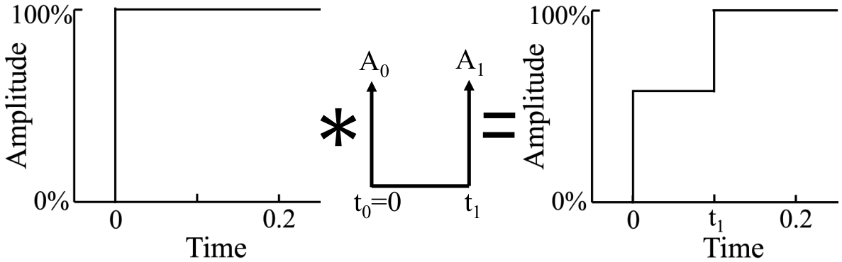
Work by Singer and Seering demonstrated that it is possible to reduce residual vibration in vibratory systems through a command generation technique called input shaping [16]. The process of input shaping works by convolving a series of impulses, called an input shaper, with an arbitrary reference command and has been applied to a variety of flexible systems [17,18,19]. Figure 1 illustrates this process for a step input reference command and a two-impulse input shaper. The modified reference command is then issued to the system. The transient and residual vibratory behavior of the system is influenced by the time and amplitude of the impulses comprising the input shaper. Using knowledge about a linear system’s natural frequency and damping ratio, it is possible to design an input shaper that eliminates residual vibration from the system’s response.

While this command shaping approach was developed using linear system theory, it has been shown to remain effective at maintaining low residual vibration even when applied to systems with low levels of nonlinear frequency and damping behavior [16,20,21,22,23,24,25]. Prior work by Schlagenhauf et al. has shown that the residual vibration reduction in input shapers extends to the nonlinear responses of LRAs [26].

Additionally, many common shapers were initially devised in the continuous time domain including the zero vibration (ZV) [16], zero vibration and derivative (ZVD) [16], extra insensitive (EI) [27], specified insensitivity (SI) [27], and modified input (MI) shapers [28]. However, to be implemented in physical systems the shaper must often be discretized. One such instance occurs when a system has a finite number of admissible actuation states that do not encompass the entire set of input-shaped command values [29,30]. Additionally, the discrete update rate of a system may not align with the oscillatory frequency of the system. This can result in impulses occurring at discrete time steps that do not align with the ideal times of the continuous-time shaper.

Two questions then naturally arise:

• What methods can be used to discretize the input shaper for use on a discrete time system?
• How does discretization diminish the effectiveness of a given input shaper’s vibration-reducing properties?

These questions have been addressed by previous researchers who focused mainly on linear systems. Their approaches for developing discrete time input shapers can generally be categorized as one or more of the following techniques:

• Numerical conversion of continuous-time shapers;
• Z-plane pole placement techniques;
• Direct solution of the input shaper design equations in the digital time domain;
• Numerical optimization of shaper parameters.

In numerical conversion the impulses of a continuous-time shaper that do not coincide with specified discrete time instances are shifted to the closest discrete time instance or instances based on the amplitude and timing of the continuous time impulses and the specific numerical conversion technique implemented. One approach to direct numerical conversion is simply shifting the impulses to occur at the nearest discrete time locations [31,32]. For high clock rate systems this approach can provide easy and accurate discrete time shapers. However, as discussed by Singer, the error associated with this approach increases as the sampling time step increases [31]. A second approach, which is examined in this paper, is to split the amplitude of the continuous time impulses between the two closest discrete time locations [32].

A number of works have examined the development of input shapers through application of z-plane techniques. Murphy and Watanabe used z-plane analysis to design an arbitrary rate digital shaping filter [33]. Tuttle and Seering then applied these z-plane techniques to the development of multi-mode discrete time input shapers [34]. While Park et al. furthered the work of Murphy and Watanabe by applying z-plane analysis to the development of more robust shaping filters and devising a discrete time sensitivity expression [35]. Seth et al. developed digital shapers using z-plane analysis to reduce vibration in coordinate measuring machines [36]. Wang and Shao later used this z-plane approach to develop symmetric and asymmetric multi-hump input shapers [37].

As detailed by Robertson et al., the input shaper design equations may be directly solved to obtain a discrete time input shaper by restricting the impulse times to fall on multiples of the sampling time [38]. However, due to the non-uniqueness of minimum time solutions Robertson et al. employed an optimization to minimize a secondary performance metric.

A number of additional works have examined the identification of discrete time input shapers through optimization techniques [39,40,41,42]. To handle higher-order, linear time-invariant systems Van den Broeck et al. applied a linear programming framework to identify discrete input shapers for different sampling rates [39]. While Kamel et al. implemented an optimization technique to identify optimal discrete time input shapers that minimize the quadratic control error associated with the desired transient motion of a robotic arm end-effector. Additionally, Hyde and Seering used a discrete time optimization technique to develop digital input shapers for the suppression of multi-mode vibration in flexible spacecraft [42].

To handle systems with position-dependent natural frequencies, Magee and Book implemented a digital shaping filter that modified the duration of the impulse sequence to account for frequency changes and verified the difficulty associated with changing the shaper duration that was predicted by Murphy and Wanatabe [43]. While, Magee used a cost function to develop an optimal arbitrary time-delay filter [44].

Additionally, Park et al. applied input shaping to a system with a natural frequency that varied during motion [45]. However, this approach required the change in system parameters to occur during a period of constant velocity. Work by Aboel-Hassan et al. demonstrated it was possible to develop effective discrete time input shapers for nonlinear systems through optimization of the first impulse amplitude and second impulse timing [46]. In addition, although nonlinearities exist due to the gradient of the electromagnetic field within the LRA, prior simulated work suggests it is possible to obtain effective discrete input shapers for a range of discretization periods [47].

This paper focuses on the effect discretization period has on the ability of various discretization methods to eliminate residual acceleration of a physical LRA system. One of the key challenges is accounting for the particular nonlinearities that arise in LRAs. These nonlinear dynamics have been studied in previous publications [8,26,47]. The effectiveness and shape of the discrete time shapers are then evaluated to develop a streamlined process for the future development of discrete time LRA input shapers.

The next section will discuss the experimental setup and procedure used to gather data. Then the discretization approaches employed will be introduced in Section 3, followed by analysis of the effectiveness of these techniques in Section 4. In addition, this work develops a strategy for obtaining discrete time input shapers capable of minimizing the acceleration ratio, the ratio of peak residual acceleration to peak–peak maximum transient acceleration, in LRAs with nonlinear frequency dynamics over a range of discretization periods. Lastly, Section 5 presents the conclusions of this work and discusses a potential streamlined process for the development of discrete time input shapers for untested discretization periods or untested LRA models.

2. Experimental Setup

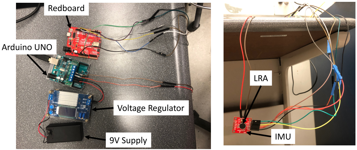
In order to investigate various discrete time shapers effectiveness on LRAs, shaped step inputs were applied to a VG1040003D Vybronics LRA (Vybronics Inc., Wenzhou, China) with a resonance frequency of 170 Hz. Acceleration data was collected using the setup shown in Figure 2. A 9 V power supply was used in combination with a voltage regulator to supply 3.5 V to the LRA, while an Arduino Uno (Arduino S.r.l., Monza, Italy) sent inputs to the suspended LRA. The suspended LRA was adhered to a SparkFun 9DoF inertial measurement unit (IMU) (SparkFun Electronics, Niwot, CO, USA) Breakout-ICM-20948 (TDK InvenSense, San Jose, CA, USA) that recorded acceleration data from the LRA. The accelerometer data from the z-axis channel of the IMU was collected by a RedBoard Artemis (SparkFun Electronics, Niwot, CO, USA). Five trials were performed for each discrete shaper tested. The ability of the discretization methods to minimize residual oscillation was evaluated by examining the average acceleration ratio of the acceleration responses over the five trials.

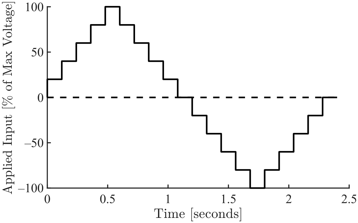
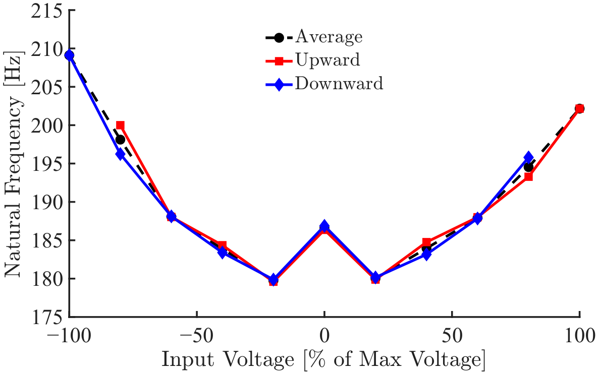
Work by Sorensen et al. has previously demonstrated that LRA frequency is dependent on the spring elongation [8]. The frequency behavior of the VG1040003D Vybronics LRA was determined by applying a series of step inputs where the applied voltage was changed by 20% of the maximum voltage, as seen in Figure 3. A Fast Fourier Transform (FFT) was then performed on the acceleration response profiles to identify the frequency of the LRA at different voltage levels. The resulting frequency response profile for all voltage steps is shown in Figure 4. The x-axis of Figure 4 represents the voltage at the end of a given step input, with positive changes in input voltage corresponding to an upward step and negative changes corresponding to a downward step.

3. Shaper Discretization Methods

The four discretization strategies examined are:

• Proportional split discretization;
• Presplit discretization;
• Extended-duration presplit discretization;
• Direct solution of vibration constraints at given discrete times.

The continuous time ZV shaper was selected to serve as the foundation for the development of the discrete input shapers implemented in this work. The two-impulse sequence of the ZV shaper is defined as [16,48]:

$$\left[\begin{array}{c}{A}_i\\ t_i\end{array}\right]=\left[\begin{array}{cc}{\displaystyle \frac{1}{1+K}}& {\displaystyle \frac{K}{1+K}}\\ 0& 0.5T_d\end{array}\right],$$

(1)

where the variable K is defined as a function of the damping ratio $\zeta$:

$$K=e^{-{\displaystyle \frac{\zeta \pi }{\sqrt{1-{\zeta }^2}}}},$$

(2)

and the damped period of oscillation $T_d$ is a function of the system’s damping ratio and natural frequency ${\omega }_n$:

$$T_d={\displaystyle \frac{2\pi }{{\omega }_n\sqrt{1-{\zeta }^2}}}.$$

(3)

Since the frequency of the LRA varies with applied voltage, the optimization approach employed by Aboel-Hassan et al. was used to determine an approximate continuous time ZV shaper for the 0 percent to 100 percent maximum voltage step [46]. The acceleration ratio, the ratio of maximum residual acceleration to maximum peak to peak transient acceleration, was used as the performance index in the optimization and the step size used to find the second impulse time was an order of magnitude smaller than the shortest discretization period investigated.

3.1. Proportional Split Method

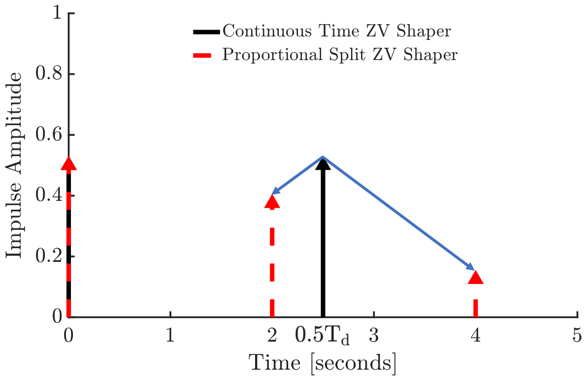
As seen in Figure 5 for a two impulse continuous time shaper the proportional split discretization method apportions the amplitude of the second impulse between the two closest discrete time instances using the expressions:

$$A_2={\displaystyle \frac{t_3-t_B}{t_3-t_2}}\times A_B,$$

(4)

$$A_3={\displaystyle \frac{t_B-t_2}{t_3-t_2}}\times A_B,$$

(5)

where $A_B$ is the amplitude of the second impulse in the continuous time shaper, and $A_2$ and $A_3$ are the amplitudes of the discrete time impulses. The time of the second impulse in the continuous time shaper is expressed as $t_B$, while $t_2$ and $t_3$ are the discrete time instances directly before and after $t_B$ respectively. These discrete time instances are respectively expressed mathematically as the product of the discretization period and the floor/ceiling of the second impulse time in the continuous shaper divided by the discretization period:

$$t_2=\lfloor {\displaystyle \frac{t_B}{t_d}}\rfloor t_d,$$

(6)

$$t_3=\lceil {\displaystyle \frac{t_B}{t_d}}\rceil t_d.$$

(7)

While proportional split discretization is simple to apply, this approach loses effectiveness as the spacing between the discrete time impulse locations and the continuous time impulse locations increases.

3.2. Presplit Method

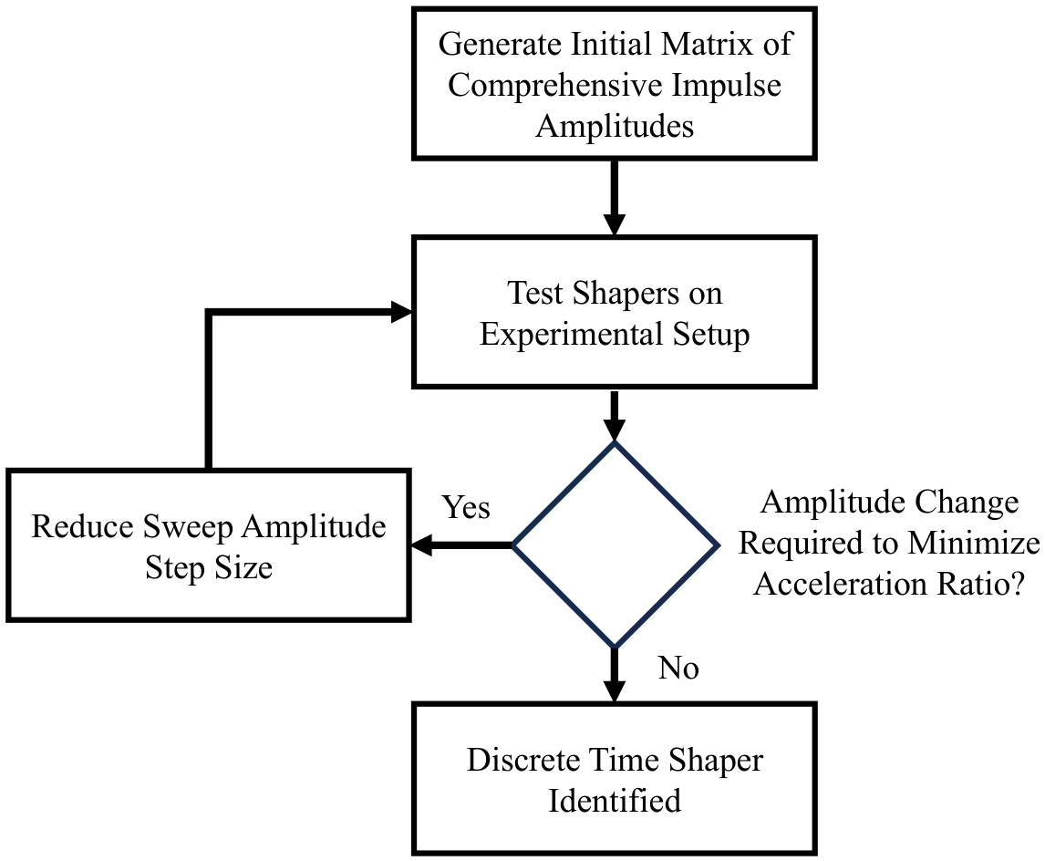
Using the same impulse times as the proportional split discretization, the amplitudes of the presplit discrete shaper are determined through a trend sweep search optimization [47]. For a discrete three-impulse shaper the amplitudes of the first two impulses convolved with the step input are varied to minimize the acceleration ratio, the ratio of acceleration overshoot after the last impulse divided by the maximum peak–peak acceleration. The identification process for discrete presplit shapers is outlined in Figure 6. In the initial sweep the amplitudes of impulses 1 and 2 were varied from 0.1 to 0.7 and 0.1 to 0.6 respectively by steps of 0.1 units. To ensure final displacement of the LRA’s internal mass remains consistent with the response of the unshaped step input reference command, the amplitude of the third impulse in the presplit shaper is restricted to a value of 1 minus the sum of the previous two impulses. Maximum values for the amplitudes of impulse 1 and 2 were constrained such that the amplitude of impulse 3 remained greater than 0. The size of steps between tested amplitudes was iteratively reduced until an identical shaper was identified in two successive sweeps. For discretization periods, $t_d$, greater than half the damped period of oscillation, the two discrete time instances closest to the time of the second impulse in the continuous time shaper, $t_B$, become $t_2=0$ and $t_3=t_d$. Thus, as both $t_1=0$ and $t_2=0$ the presplit shaper effectively reduces to a two-impulse discrete shaper for discretization periods greater than half the damped period of oscillation. To maintain a shaper whose amplitudes sum to 1, only the amplitude of the first impulse is optimized and the amplitude of the second impulse becomes 1 minus the amplitude of the first impulse.

3.3. Extended-Duration Presplit Method

Extended-duration discretization increases the range of discretization periods that can minimize residual acceleration at the expense of a longer response time. For discretization periods above half the damped period of oscillation the extended-duration presplit method places impulses at times of zero, the discretization period and two times the discretization period, as seen in the expression [47]:

$$\left[\begin{array}{ccc}{A}_1& A_2& 1-(A_1+A_2)\\ 0& t_d& 2\times t_d\end{array}\right].$$

(8)

As with the presplit method, the amplitudes of the impulses in the extended-duration presplit shaper are determined through a trend sweep search optimization outlined in Figure 6.

3.4. Direct Solution of Vibration Constraints

Direct solution of discrete time ZV shapers is possible by restricting the impulse times, $t_i$, in the vibration constraint equations [38]:

$$V({\omega }_n,\zeta )=0=e^{-\zeta {\omega }_n{t}_n}\sqrt{{\left[C({\omega }_n,\zeta )\right]}^2+{\left[S({\omega }_n,\zeta )\right]}^2},$$

(9)

where $t_n$ is the time of the last impulse and

$$C({\omega }_n,\zeta )={\displaystyle \sum _{i=1}^N}{A}_i{e}^{\zeta {\omega }_n{t}_i}cos\left({\omega }_d{t}_i\right),$$

(10)

and

$$S({\omega }_n,\zeta )={\displaystyle \sum _{i=1}^N}{A}_i{e}^{\zeta {\omega }_n{t}_i}sin\left({\omega }_d{t}_i\right),$$

(11)

where N is the number of impulses in the shaper and ${\omega }_d$ is the damped frequency of the system. This restriction of the impulse times to known discrete time values turns (10) and (11) into linear equations of impulse amplitude $A_i$.

For discrete shapers where the number of impulses is three, the additional constraint that impulse amplitudes sum to one enables these equations to be expressed in the matrix form:

$$\left[\begin{array}{ccc}1& 1& 1\\ 1& e^{\zeta {\omega }_n{t}_2}cos\left({\omega }_d{t}_2\right)& e^{\zeta {\omega }_n{t}_3}cos\left({\omega }_d{t}_3\right)\\ 0& e^{\zeta {\omega }_n{t}_2}sin\left({\omega }_d{t}_2\right)& e^{\zeta {\omega }_n{t}_3}sin\left({\omega }_d{t}_3\right)\end{array}\right]\left(\begin{array}{c}{A}_1\\ A_2\\ A_3\end{array}\right)=\left(\begin{array}{c}1\\ 0\\ 0\end{array}\right).$$

(12)

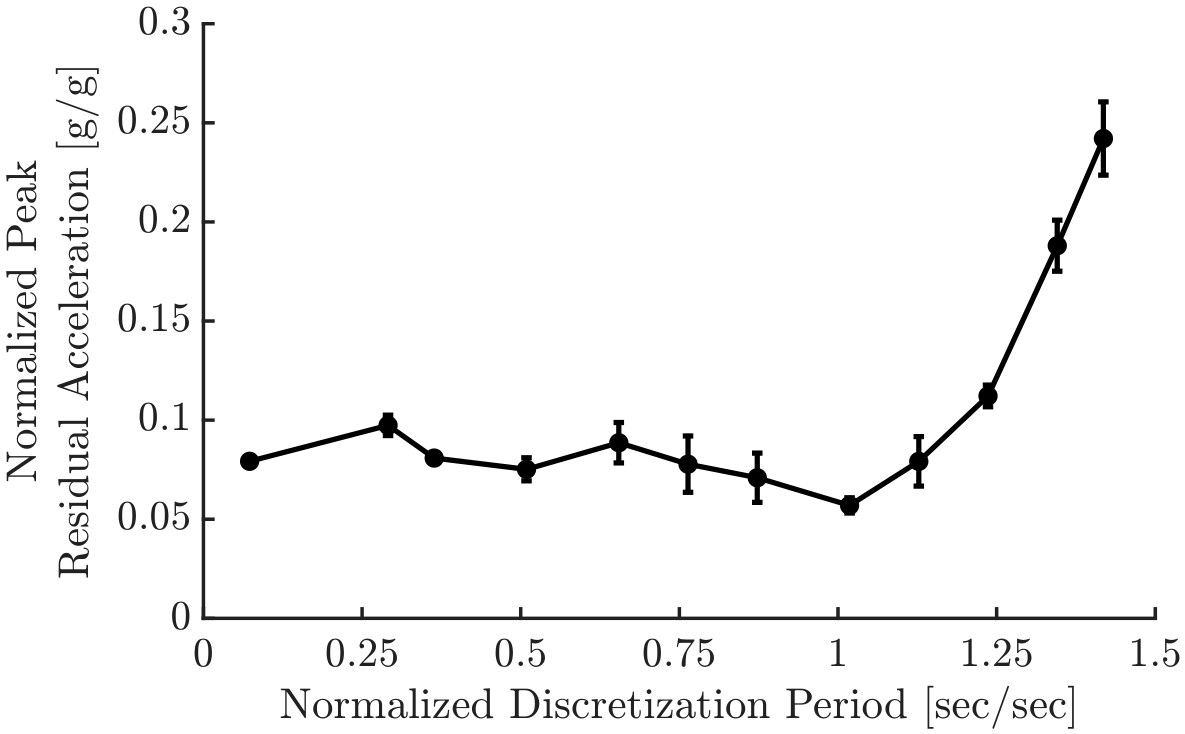
The impulse amplitudes may then be determined through matrix inversion so long as discrete times of the second and third impulses, $t_2$ and $t_3$, are chosen such that the matrix is non-singular. However due to the nonlinearity of the LRAs the effectiveness of this approach is limited, as seen by the five-trial average peak residual acceleration normalized by the maximum absolute acceleration of the unshaped response in Figure 7, where the discretization period is normalized by the second impulse time of a continuous time two-impulse shaper optimized for the LRA using a trend sweep search. The peak residual acceleration of the input-shaped response was taken as the largest acceleration reading for a period of roughly 0.12 s after the last impulse. Error bars in Figure 7 and subsequent plots are included to show one standard deviation of uncertainty in the five trial averages.

4. Results

4.1. Proportional Split vs. Presplit

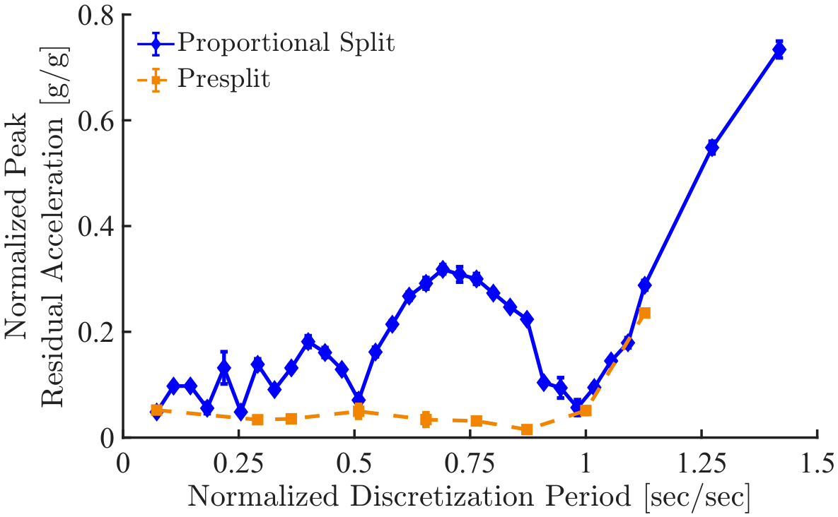
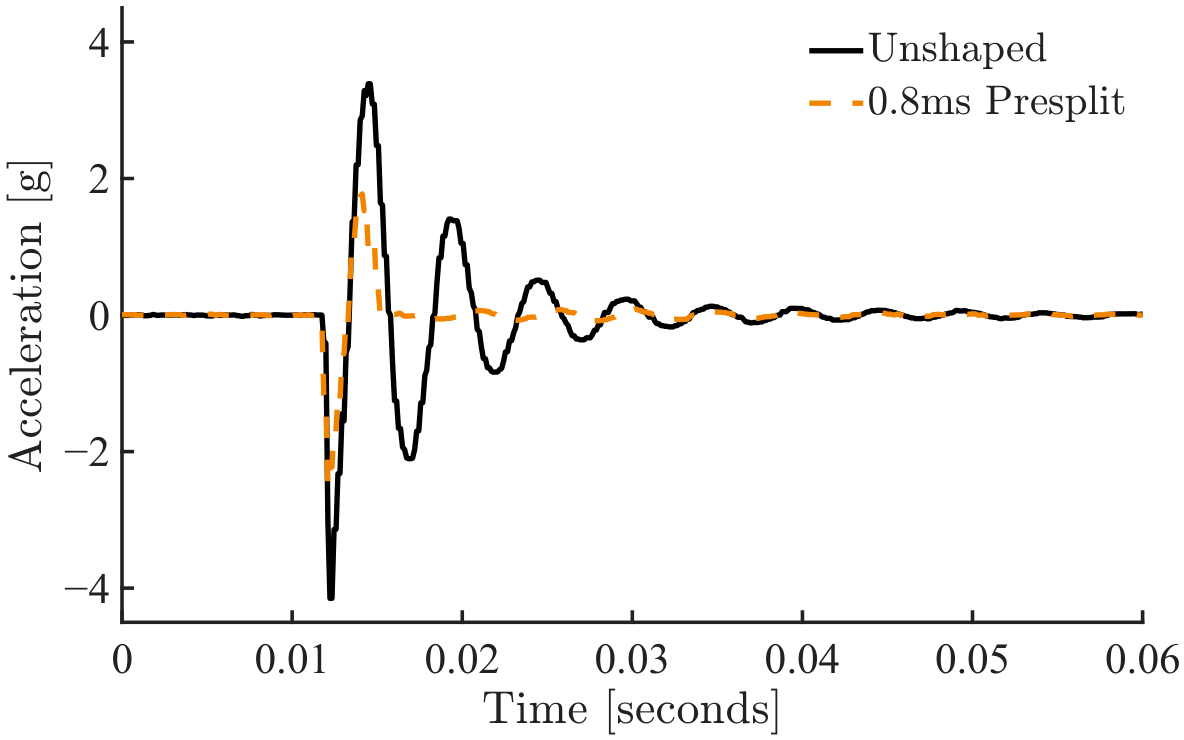
The normalized average peak residual acceleration over five trials for the proportional split and presplit methods is shown in Figure 8. Although the presplit method yields effective reduction in residual acceleration, as seen in Figure 8, the maximum acceleration generated by the LRA is also reduced, as seen in Figure 9 for a presplit shaper with a discretization period of 0.8 ms. This reduction can limit the effectiveness of the haptic effect [49].

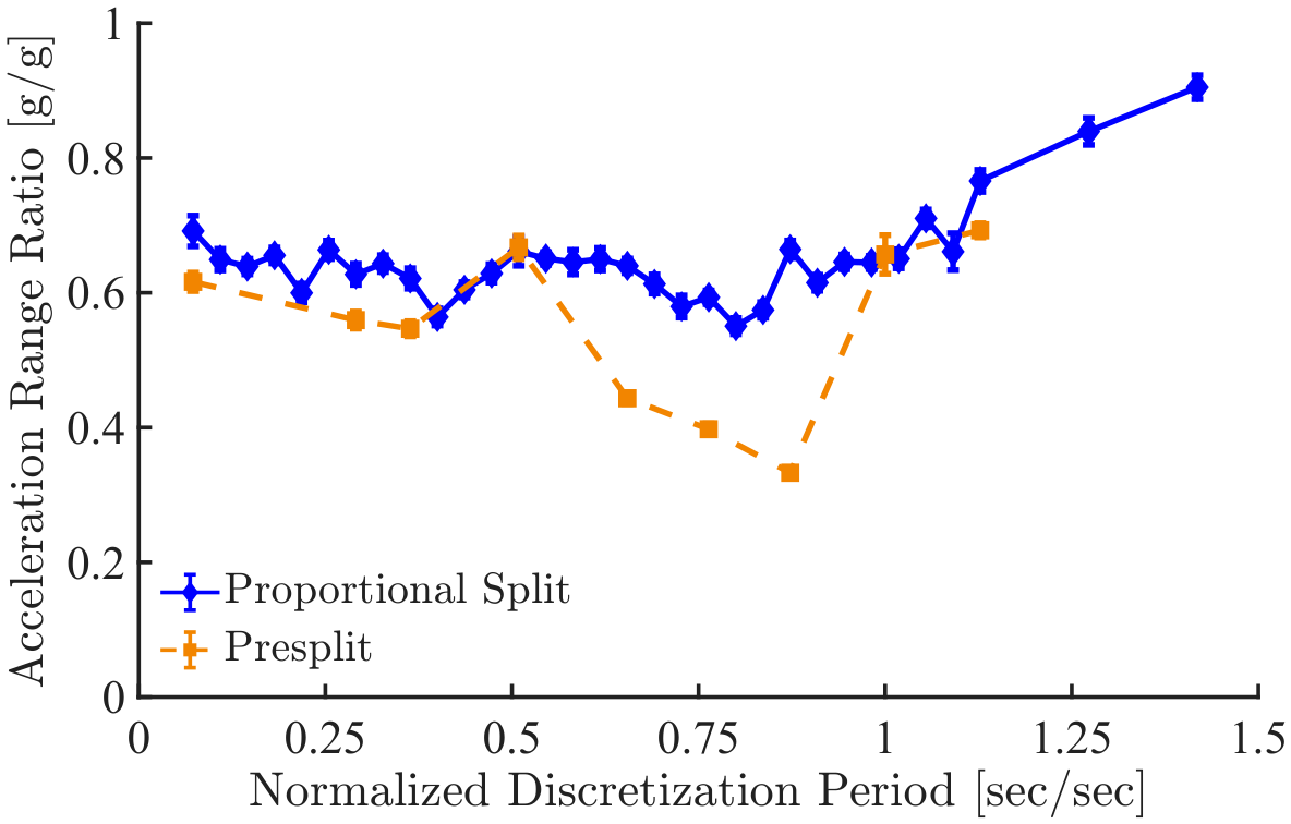
For applications of interest it is generally desirable to generate several large initial acceleration values over a desired time period then cancel out all residual oscillation. Therefore, normalized peak residual acceleration is an insufficient tool for evaluating the effectiveness of the discretization methods as it does not account for the reduction in the maximum peak–peak acceleration. Figure 10 shows this reduction through the ratio of the acceleration range of the proportional split and presplit responses to the acceleration range of the unshaped response versus the normalized discretization period. For the tested discretization periods the reduction in acceleration range resulting from the presplit shaping of the step input ranges from a 30% reduction to a 67% reduction, while the proportional split shaper sees reductions ranging from 10% to 41%. Thus, while the presplit shaper is more effective at minimizing residual oscillation for a wider range of discretization periods, it also tends to produce smaller peak–peak accelerations during the transient phase than the proportional split shaper. By dividing the peak residual acceleration of the response by the maximum peak–peak acceleration the acceleration ratio acts as an effective tool for evaluating the effectiveness of the discretized shapers in the context of generating haptic effects with LRAs.

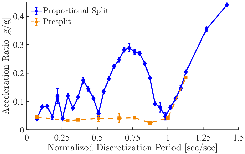
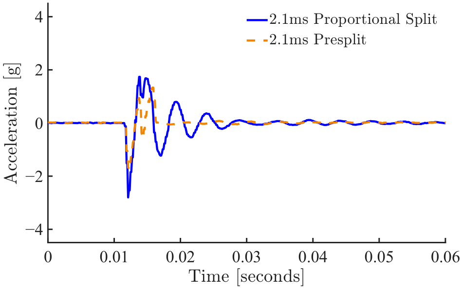
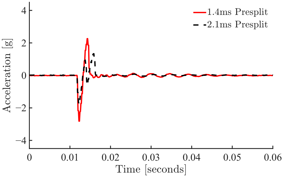
The average acceleration ratio over five trials versus the discretization period normalized by half the damped period of oscillation for the proportional split and presplit methods is shown in Figure 11. The presplit method was able to minimize the acceleration ratio up to a normalized discretization period of 1. The proportional split method was effective at minimizing the acceleration ratio when the normalized discretization period was small or close to 0.5 or 1. However, this method became ineffective as the normalized discretization period moved toward 0.75. The acceleration responses for these two methods for a normalized discretization period of 0.764 (2.1 ms) are shown in Figure 12. Although the proportional split yields larger peak–peak acceleration it takes significantly longer to settle than the presplit method. In addition, even though the presplit method was able to minimize the acceleration ratio for the normalized discretization periods below 1 the acceleration response profiles varied with the discretization period. As seen in Figure 13 the acceleration responses for normalized discretization periods of 0.509 (1.4 ms) and 0.764 both settle quickly; however, the maximum peak–peak acceleration for the normalized discretization period of 0.509 is roughly 5 g while it is only 3 g for the normalized discretization period of 0.764.

4.2. Coarse Discretization Periods

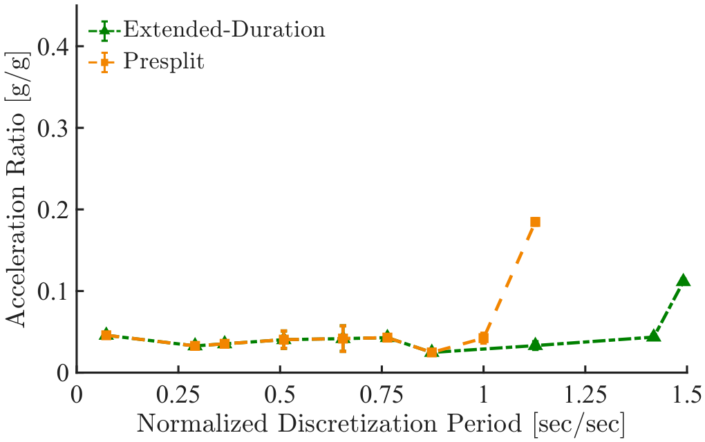
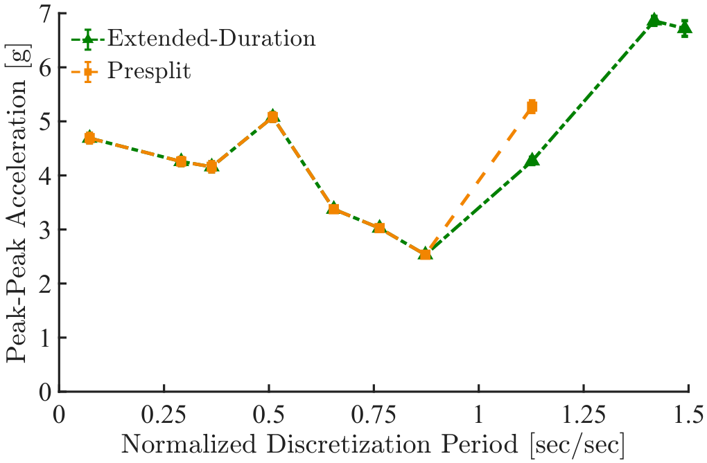
As the normalized discretization period rises above 0.5 the timing of the impulses in the discrete shaper begins to resemble a continuous time ZVD shaper where the third impulse occurs at two times the time of the second impulse. On the other hand, as the normalized discretization period rises above 1 the number of impulses in the discrete shaper decreases from three to two, which is more consistent with the structure of a continuous time ZV shaper. This drop in shaper length corresponds with a sharp decrease in shaper effectiveness for both the proportional split and presplit methods. Examining the acceleration ratio of proportional split shapers with normalized discretization periods close to 1 in Figure 11 it is evident that discretization periods slightly less than half the damped period of oscillation yielded slightly more effective proportional split shapers than discretization periods greater than half the damped period of oscillation. While this improvement was minor for the proportional split method with differences in acceleration ratio between discretization periods of $0.5T_d-t_D$ and $0.5T_d+t_D$ around 0.02 to 0.05, where $t_D$ is the absolute value of the difference in time between $0.5T_d$ and the discretization period, the difference was significant for the presplit method. By extending the duration of the shaper such that the discrete shaper has three impulses when the normalized discretization period is greater than 1 it is possible to increase the range of discretization periods that can be employed while still minimizing the acceleration ratio, as seen in Figure 14.

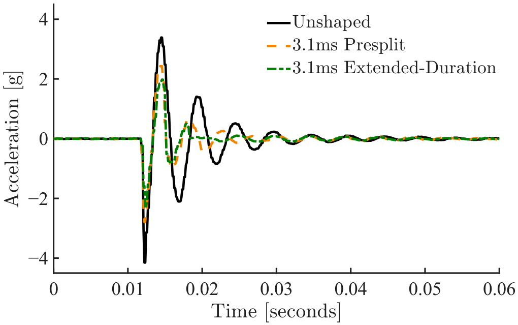
Figure 15 shows the acceleration response of the LRA to a step input shaped by a presplit shaper and an extended-duration shaper versus the unshaped response for a normalized discretization period of 1.127 (3.1 ms).

Although the presplit and extended-duration methods are able to minimize the acceleration ratio for normalized discretization periods below 1, the peak–peak maximum acceleration varies with the discretization period as seen in Figure 16. For discretization periods less than a quarter of the damped period of oscillation the maximum peak–peak acceleration changes little as the amplitude of the first impulse remains relatively constant for these discretization periods. However, above a normalized discretization period of 0.5 the amplitude of the first impulse for both methods varies yielding a wide range of peak–peak acceleration values. Above a normalized discretization period of 1 the presplit shaper is no longer identical to the extended-duration shaper and the peak–peak accelerations for the two approaches diverge.

4.3. Optimized vs. Approximate Presplit Shapers

Obtaining approximate expressions for the relationship between impulse time and amplitude for the presplit shapers would enable accelerated development of presplit shapers for additional untested discretization periods by narrowing down the range of impulse amplitudes used in the initial trend sweep search optimization.

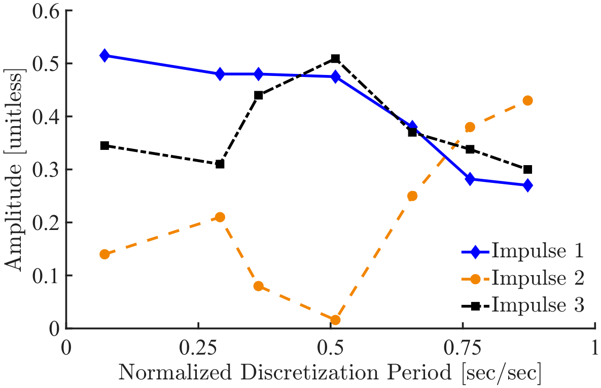
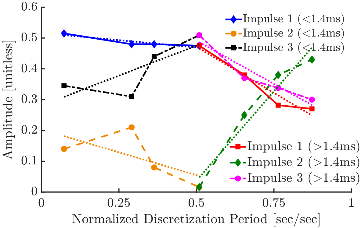
Figure 17 shows the amplitudes of the three impulses in the presplit shapers for normalized discretization periods ranging from 0.072 to 0.872. Segmenting this data into two parts, discretization periods above 0.5 and discretization periods below 0.5, two trendlines can be fit to the data for each impulse and are depicted in Figure 18 with dotted lines. As seen in Figure 18 these trendlines fit well for normalized discretization periods in the 0.5 to 1 range yielding $R^2$ values of 0.9436, 0.9506, and 0.9172 for impulses one, two, and three respectively; however, they fit poorly for normalized discretization periods in the 0 to 0.5 range particularly for impulses two and three where the $R^2$ values fell to 0.6112 and 0.421.

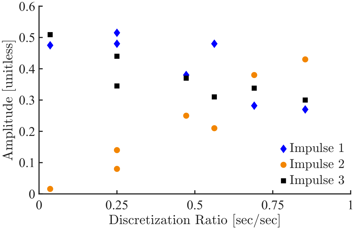
As seen by (4) and (5) the second and third impulses of the proportional split shaper have a linear relation with the impulse time ratios. The impulse amplitudes of the presplit shaper plotted against the discretization ratio:

$$d_r={\displaystyle \frac{t_3-t_B}{t_3-t_2}},$$

(13)

are seen in Figure 19. Substituting in (6) and (7) the discretization ratio is expressed as a function of the discretization period:

$$d_r\left(t_d\right)={\displaystyle \frac{\lceil \frac{t_B}{t_d}\rceil t_d-t_B}{\lceil \frac{t_B}{t_d}\rceil t_d-\lfloor \frac{t_B}{t_d}\rfloor t_d}}.$$

(14)

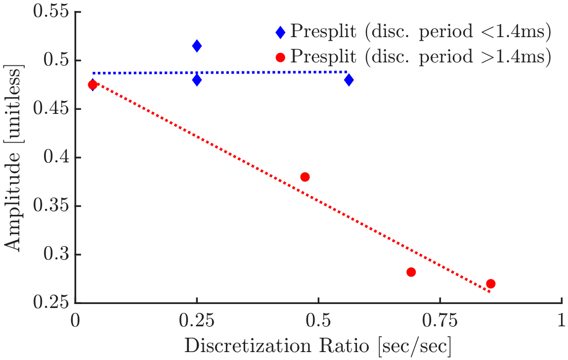
Segmenting the amplitude data then yields two distinct well-fit linear trendlines for the first impulse amplitude seen in Figure 20, with one trendline representing discretization periods less than a quarter the damped period of oscillation, while the second represents discretization periods between one quarter and half the damped period of oscillation. In Figure 20 these trendlines, and those in subsequent plots, are depicted as dotted lines.

For shapers with discretization periods below one quarter the damped period of oscillation ($t_d$ < 1.4 ms) the relation between the discretization ratio, $d_r$, and the amplitude of the first impulse of the discrete shaper, $A_1$, is approximated by the expression:

$$A_1=0.0024d_r+0.4868,$$

(15)

while the relationship between the discretization ratio and the amplitude of the first impulse for discretization periods between one quarter and half the damped period of oscillation (1.4 ms < $t_d$ < 2.8 ms) is approximated by the expression:

$$A_1=-0.2657d_r+0.4881.$$

(16)

The $R^2$ value for the linear approximation of the greater than 0.5 normalized discretization period case increases to 0.9671.

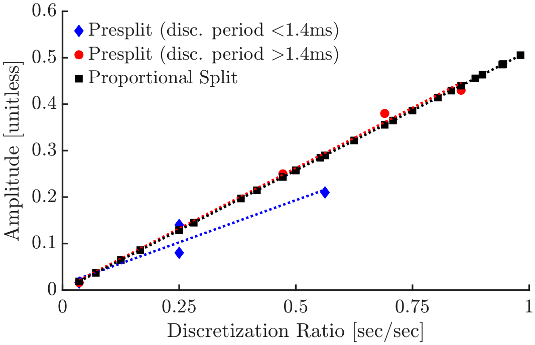
Similar relations between the discretization ratio and impulse amplitude can be seen for the second and third impulses in presplit shapers when amplitude data is segmented such that one set reflects discretization periods less than a quarter the damped period of oscillation, while the second represents discretization periods between one quarter and half the damped period of oscillation. Figure 21 shows the discretization ratio versus the second impulse amplitudes of presplit shapers and proportional split shapers with varying discretization periods. For presplit shapers with discretization periods less than one quarter the damped period of oscillation ($t_d$ < 1.4 ms) an approximation of the relationship between discretization ratio and the second impulse amplitude is given by the equation:

$$A_2=0.363d_r+0.0118,$$

(17)

while a linear approximation of the relationship between discretization ratio and the second impulse amplitude for presplit shapers with discretization periods between one quarter and half the damped period of oscillation (1.4 ms < $t_d$ < 2.8 ms) is given by:

$$A_2=0.5198d_r+0.0023.$$

(18)

The $R^2$ values for these linear approximations rose from 0.6112 to 0.9019 for the less than 0.5 normalized discretization period case and 0.9506 to 0.9937 for the greater than 0.5 case. The amplitude of the second impulse in the proportional split shapers is obtained through (4).

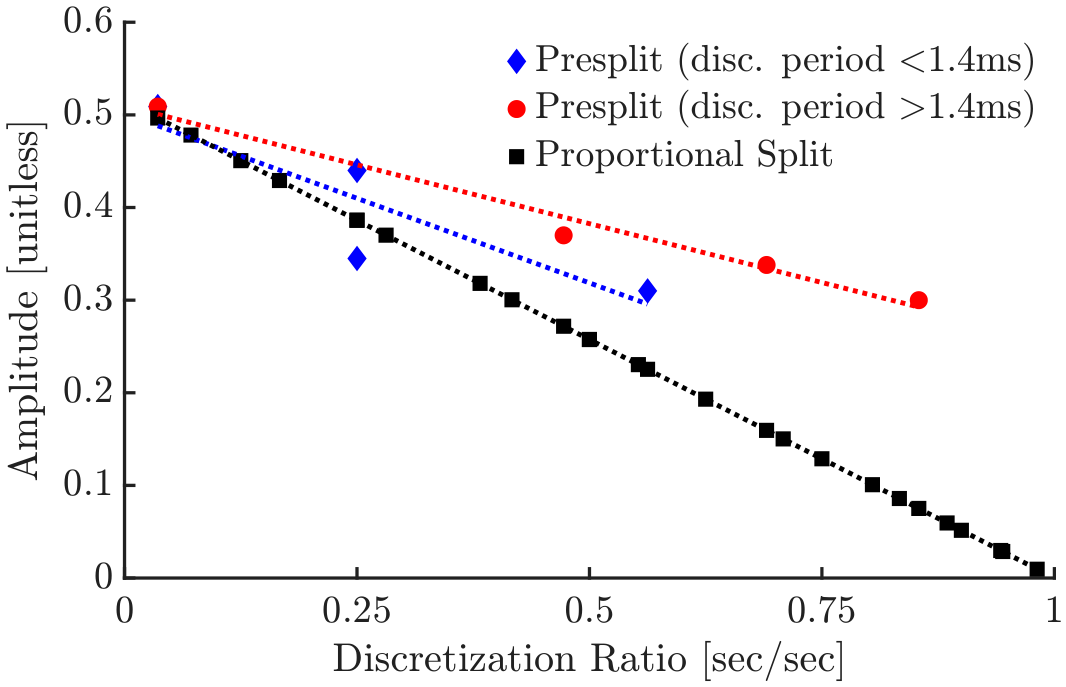
Lastly, the relationship between the discretization ratio and the amplitude of the third impulse in the discrete presplit shapers is shown in Figure 22. Similar to impulses one and two, two linear approximations of the relationship between discretization ratio and impulse amplitude can be obtained. For discretization periods less than one quarter the damped period of oscillation ($t_d$ < 1.4 ms), this relationship is approximated as:

$$A_3=-0.3654d_r+0.5013,$$

(19)

while for discretization ratios between one quarter and half the damped period of oscillation (1.4 ms < $t_d$ < 2.8 ms) this relationship is approximated by the expression:

$$A_3=-0.2542d_r+0.5097.$$

(20)

For these linear approximations the $R^2$ values rose to 0.7661 and 0.9789 for the less than 0.5 and greater than 0.5 normalized discretization period cases from values of 0.421 and 0.9172 for the linear approximations seen in Figure 18. As the third-impulse amplitude is a function of the first two-impulse amplitudes, the difference in amplitude from the linear trendline is propagated when calculating the third impulse amplitude resulting in lower $R^2$ values compared to impulses one and two. The amplitudes for the third impulse of the proportional split shapers shown in Figure 22 are calculated from (5).

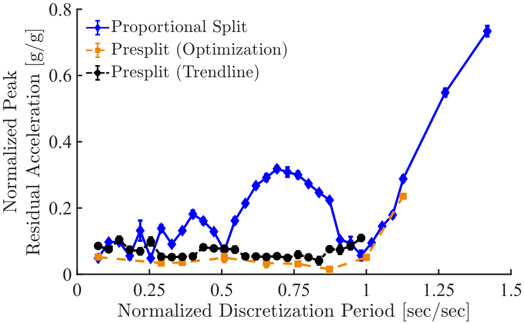
To test the effectiveness of these linear trendlines, approximate presplit shapers were developed for discretization periods ranging from 0.2 ms to 2.7 ms using Equations (15)–(20). Figure 23 shows the normalized peak residual acceleration for approximate and optimized presplit shapers, and proportional split shapers. Although the presplit shapers derived from the linear approximation expressions were less effective at minimizing residual acceleration than the presplit shapers obtained through the trend sweep optimization, they were able to keep the normalized residual acceleration below 0.1 for discretization periods up to 2.7 ms.

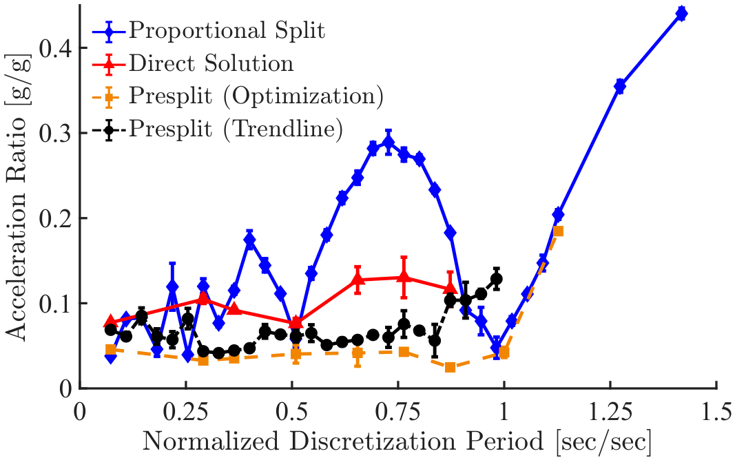
The trendline presplit approximation method yielded smaller peak–peak maximum acceleration values than the optimized presplit shapers resulting in larger acceleration ratio values as seen in Figure 24. Although the presplit shapers derived from the linear approximation expressions resulted in smaller peak–peak acceleration values they managed to hold the acceleration ratio below 0.1 for discretization periods up to 2.3 ms and below 0.13 for discretization periods up to 2.7 ms. The approximated presplit shapers also yielded reduced acceleration ratios for most discretization periods tested when compared to the proportional split method.

4.4. Direct Solution of Constraints vs. Approximate Presplit Shapers

While the approximate presplit shaper expressions are an effective starting point for optimization of additional discretization periods it requires the optimization of at least three discrete presplit shapers to obtain amplitude expressions.

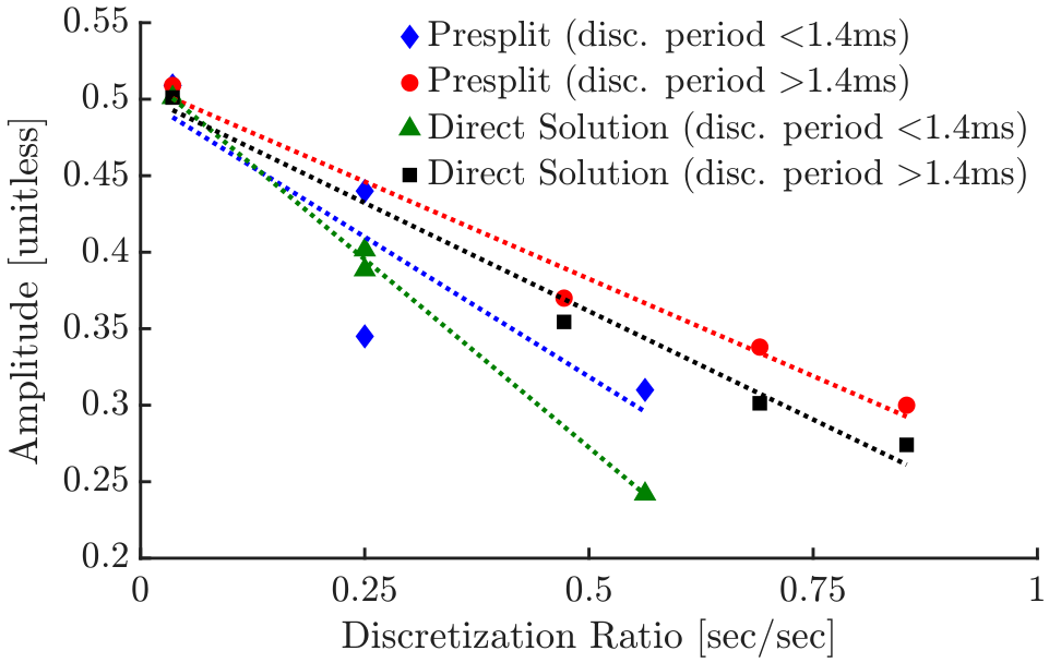
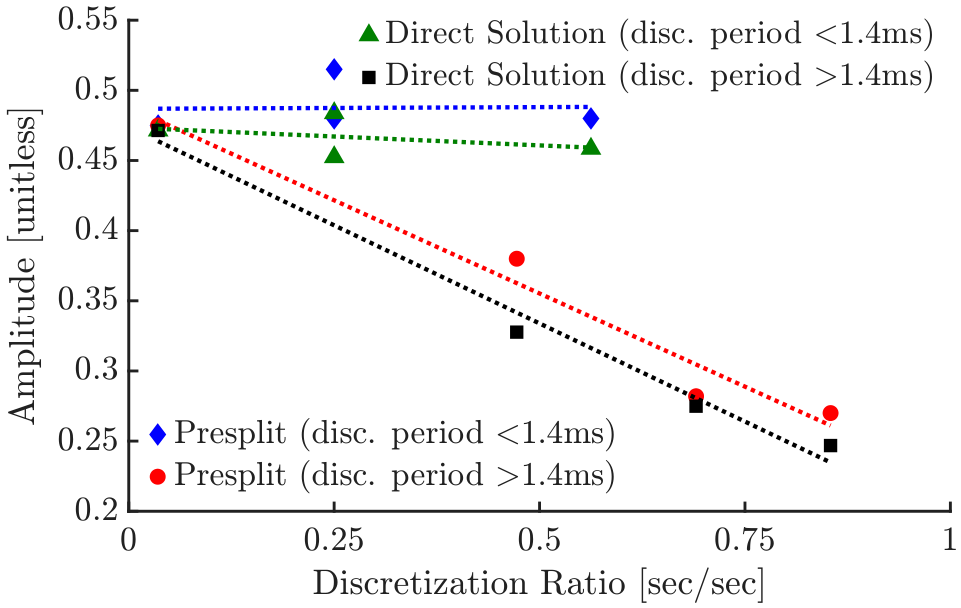
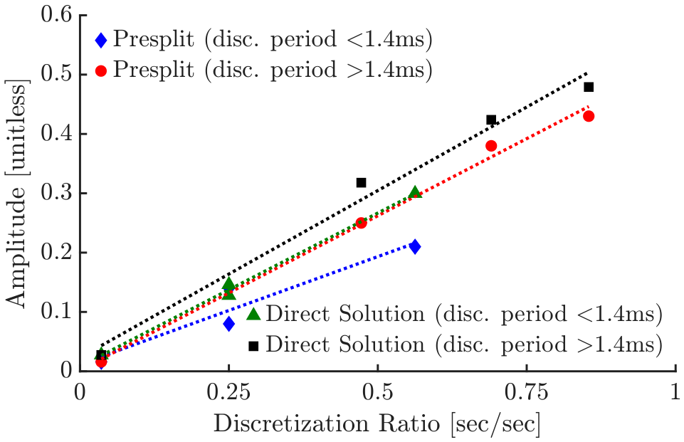
As seen in Figure 22 the proportional split method only yields discrete shapers with amplitudes similar to presplit shapers when the discretization ratio is small making it an ineffective starting point for optimization of presplit shapers for a wide range of discretization periods. However, applying the direct solution of constraints approach, it is possible to determine rough estimates of effective impulse amplitudes before optimizing any presplit shapers. While the direct solution of vibration constraint equations to determine discrete shaper amplitudes yields larger acceleration ratios than either the optimized presplit or trendline presplit approximation methods, as seen in Figure 24, the relationship between impulse amplitude and discretization ratio for the direct solution discrete shapers closely matches the presplit trendline approximation. Figure 25 shows this correlation for the first impulse amplitude, while Figure 26 and Figure 27 show this relationship for the second and third impulses of the discrete shapers. Thus, it is possible to use the direct solution of discrete shapers to narrow down the range of possible amplitudes for the optimized presplit shaper, decreasing optimization time.

5. Conclusions

This paper investigated how the discretization period affects the ability of four discretization methods to minimize the acceleration ratio of a VG1040003D Vybronics LRA driven by shaped inputs. While the effectiveness of the proportional split method varied significantly with discretization period, by selecting a normalized discretization period with a multiple close to 1 it was possible to minimize the acceleration ratio of the response. Implementation of the presplit method resulted in responses with minimized acceleration ratios up to a normalized discretization period of 1; however, the maximum peak–peak acceleration still varied with discretization period and was reduced greatly from the unshaped case. By enforcing the condition that the number of impulses must remain three irrespective of the discretization period, the extended-duration method yielded a larger range of discretization periods that could minimize the acceleration ratio.

While the presplit and extended-duration methods were effective, they required optimization for each new discretization period of interest. Solving the vibration constraint equations directly for a set of discrete impulse times and using the natural frequency and damping ratio that yielded the continuous time shaper it was possible to obtain estimates for the amplitudes of a three-impulse discrete time shaper. Although the effectiveness of the direct solution of constraints approach is limited due to the nonlinearity of the system dynamics it does narrow down the range of amplitudes that may provide effective residual vibration reduction and reduce the amount of optimization required to obtain effective presplit shapers.

Furthermore, by plotting the impulse amplitudes of the presplit shapers versus discretization ratio and splitting the data into two sets, one for discretization periods less than one quarter the damped period of oscillation and the other set for discretization periods between one quarter and one half the damped period of oscillation, it was possible to obtain linear expressions for impulse amplitude. The resulting approximate presplit shapers yielded improved vibration reduction in comparison to the direct solution of constraints for discrete shapers. In addition, the approximate presplit shapers provided better estimates for the impulse amplitudes of the optimized presplit shapers.

These results suggest the development of effective input shapers is possible for a 0 to 100% voltage step applied to the investigated LRA and present a potential pipeline for the future development of effective input shapers at untested discretization periods. However, prior to application in haptic profiles it will be necessary to investigate how the presented discretization techniques work on different LRAs. Additionally, during haptic communication a user will often exert a force on the oscillator. Thus, future work should investigate the impact of loading on the performance for the various discretization techniques presented in this work.

References

1. Basdogan, C.; Giraud, F.; Levesque, V.; Choi, S. A Review of Surface Haptics: Enabling Tactile Effects on Touch Surfaces. IEEE Trans. Haptics 2020, 13, 450–470. [Google Scholar] [CrossRef] [Scilit] [PubMed]
2. Liu, S.H.; Kao, Y.C.; Feng, G.H. Linear Resonator Actuator-Constructed Wearable Haptic System with the Application of Converting Remote Grinding Force to Vibratory Sensation. Actuators 2023, 12, 359. [Google Scholar] [CrossRef] [Scilit]
3. Pyo, D.; Yang, T.H.; Ryu, S.; Kwon, D.S. Novel linear impact-resonant actuator for mobile applications. Sens. Actuators A Phys. 2015, 233, 460–471. [Google Scholar] [CrossRef] [Scilit]
4. Dementyev, A.; Olwal, A.; Lyon, R.F. Haptics with Input: Back-EMF in Linear Resonant Actuators to Enable Touch, Pressure and Environmental Awareness. In Proceedings of the 33rd Annual ACM Symposium on User Interface Software and Technology, New York, NY, USA, 20–23 October 2020; UIST ’20. pp. 420–429. [Google Scholar] [CrossRef] [Scilit]
5. Lindsay, J.; Adams, R.J.; Hannaford, B. Improving tactile feedback with an impedance adapter. In Proceedings of the 2013 World Haptics Conference (WHC), Daejeon, Republic of Korea, 14–17 April 2013; pp. 713–718. [Google Scholar] [CrossRef] [Scilit]
6. Won, J.; Ko, K.; Eom, H.; Kim, C.; Cho, J.; Kim, H. A Numerical Study of the Vibration Characteristics of a Haptic Actuator for a Dial Gear Shifter. Appl. Sci. 2024, 14, 9242. [Google Scholar] [CrossRef] [Scilit]
7. Cho, Y. Sensorless Resonance Tracking of Resonant Electromagnetic Actuator through Back-EMF Estimation for Mobile Devices. arXiv 2018, arXiv:1803.07065. [Google Scholar]
8. Sorensen, K.; Schmidt, R.; Jenkins, A.; Lyman, C.; Singhose, W.; Schlagenhauf, F.; Dobson, K. Electromagnetic Model of Linear Resonant Actuators. J. Dyn. Syst. Meas. Control 2023, 145, 051003. [Google Scholar] [CrossRef] [Scilit]
9. Jenkins, A. Control of Haptic Motors for Intuitive Touch Sensation. Ph.D. Thesis, Woodruff School of Mechanical Engineering, Georgia Institute of Technology, Atlanta, GA, USA, 2025. [Google Scholar]
10. Yang, Y.; Liu, C.; Chen, L.; Zhang, X. Phase deviation of semi-active suspension control and its compensation with inertial suspension. Acta Mech. Sin. 2024, 40, 523367. [Google Scholar] [CrossRef] [Scilit]
11. Vaughan, J.; Singhose, W.; Sadegh, N. A Multiple-Model Approach to Payload Compensation via Active Suspension Control. IFAC Proc. Vol. 2004, 37, 571–576. [Google Scholar] [CrossRef] [Scilit]
12. Hrovat, D. Survey of Advanced Suspension Developments and Related Optimal Control Applications. Automatica 1997, 33, 1781–1817. [Google Scholar] [CrossRef] [Scilit]
13. Campos, J.; Davis, L.; Lewis, F.L.; Ikenaga, S.; Scully, S.; Evans, M. Active suspension control of ground vehicle heave and pitch motions. In Proceedings of the 7th IEEE Mediterranean Control Conference on Control and Automation, Haifa, Israel, 28–30 June 1999; pp. 222–233. [Google Scholar]
14. Vinodh Kumar, E.; Jerome, J. Robust LQR Controller Design for Stabilizing and Trajectory Tracking of Inverted Pendulum. Procedia Eng. 2013, 64, 169–178. [Google Scholar] [CrossRef] [Scilit]
15. Prasad, L.B.; Tyagi, B.; Gupta, H.O. Optimal control of nonlinear inverted pendulum dynamical system with disturbance input using PID controller and LQR. In Proceedings of the 2011 IEEE International Conference on Control System, Computing and Engineering, Penang, Malaysia, 25–27 November 2011; pp. 540–545. [Google Scholar] [CrossRef] [Scilit]
16. Singer, N.C.; Seering, W.P. Preshaping Command Inputs to Reduce System Vibration. J. Dyn. Syst. Meas. Control 1990, 112, 76–82. [Google Scholar] [CrossRef] [Scilit]
17. Tuttle, T.D.; Seering, W.P. Experimental Verification of Vibration Reduction in Flexible Spacecraft Using Input Shaping. J. Guid. Control. Dyn. 1997, 20, 658–664. [Google Scholar] [CrossRef] [Scilit] [PubMed]
18. Mun, J.I.; Jo, T.; Kim, T.; Pahk, H.J. Residual vibration reduction of white-light scanning interferometry by input shaping. Opt. Express 2015, 23, 464–470. [Google Scholar] [CrossRef] [Scilit] [PubMed]
19. Kasprowiak, M.; Parus, A.; Hoffmann, M. Vibration Suppression with Use of Input Shaping Control in Machining. Sensors 2022, 22, 2186. [Google Scholar] [CrossRef] [Scilit] [PubMed]
20. Li, T.; Xiao, T. Physics-Informed Neural Network-Based Input Shaping for Vibration Suppression of Flexible Single-Link Robots. Actuators 2025, 14, 14. [Google Scholar] [CrossRef] [Scilit]
21. Borovic, B.; Liu, A.Q.; Popa, D.; Cai, H.; Lewis, F.L. Open-loop versus closed-loop control of MEMS devices: Choices and issues. J. Micromech. Microeng. 2005, 15, 1917. [Google Scholar] [CrossRef] [Scilit]
22. Daqaq, M.F.; Reddy, C.K.; Nayfeh, A.H. Input-shaping control of nonlinear MEMS. Nonlinear Dyn. 2008, 54, 167–179. [Google Scholar] [CrossRef] [Scilit]
23. Kinceler, R.; Meckl, P. Input shaping for nonlinear systems. In Proceedings of the 1995 American Control Conference-ACC’95, Seattle, WA, USA, 21–23 June 1995; Volume 1, pp. 914–918. [Google Scholar] [CrossRef] [Scilit]
24. Wilbanks, J.J.; Adams, C.J.; Leamy, M.J. Two-scale command shaping for feedforward control of nonlinear systems. Nonlinear Dyn. 2018, 92, 885–903. [Google Scholar] [CrossRef] [Scilit]
25. Gorinevsky, D.; Vukovich, G. Nonlinear Input Shaping Control of Flexible Spacecraft Reorientation Maneuver. J. Guid. Control. Dyn. 1998, 21, 264–270. [Google Scholar] [CrossRef] [Scilit] [PubMed]
26. Schlagenhauf, F.; Singhose, W.; Sorensen, K.; Dobson, K. Command-Shaping Control of Linear Resonant Actuators for Haptic Force Generation. IFAC-PapersOnLine 2020, 53, 8675–8682. [Google Scholar] [CrossRef] [Scilit]
27. Singhose, W. Command shaping for flexible systems: A review of the first 50 years. Int. J. Precis. Eng. Manuf. 2009, 10, 153–168. [Google Scholar] [CrossRef] [Scilit]
28. Shan, J.; Liu, H.T.; Sun, D. Modified input shaping for a rotating single-link flexible manipulator. J. Sound Vib. 2005, 285, 187–207. [Google Scholar] [CrossRef] [Scilit]
29. Peláez, G.; Singhose, W.E. Implementation of Input Shaping on Flexible Machines with Integer Controllers. IFAC Proc. Vol. 2002, 35, 37–42. [Google Scholar] [CrossRef] [Scilit]
30. Rogers, K.; Seering, W. Input shaping for limiting loads and vibration in systems with on-off actuators. In Proceedings of the American Institute of Aeronautics and Astronautics (AIAA) Guidance, Navigation, and Control Conference, San Diego, CA, USA, 29–31 July 1996. [Google Scholar] [CrossRef] [Scilit]
31. Singer, N. Residual Vibration Reduction in Computer Controlled Machines. Ph.D. Thesis, Massachusetts Institute of Technology, Cambridge, MA, USA, 1989. [Google Scholar]
32. Rappole, B. Minimizing Residual Vibrations in Flexible Systems. Master’s Thesis, Massachusetts Institute of Technology, Cambridge, MA, USA, 1992. [Google Scholar]
33. Murphy, B.; Watanabe, I. Digital shaping filters for reducing machine vibration. IEEE Trans. Robot. Autom. 1992, 8, 285–289. [Google Scholar] [CrossRef] [Scilit]
34. Tuttle, T.; Seering, W. A zero-placement technique for designing shaped inputs to suppress multiple-mode vibration. In Proceedings of the 1994 American Control Conference-ACC ’94, Baltimore, MD, USA, 29 June–1 July 1994; Volume 3, pp. 2533–2537. [Google Scholar] [CrossRef] [Scilit]
35. PARK, U.H.; LEE, J.W.; LIM, B.D.; SUNG, Y.G. Design and Sensitivity Analysis of an Input Shaping Filter in the Z-Plane. J. Sound Vib. 2001, 243, 157–171. [Google Scholar] [CrossRef] [Scilit]
36. Seth, N.; Rattan, K.; Brandstetter, R. Vibration control of a coordinate measuring machine. In Proceedings of the First IEEE Conference on Control Applications, Dayton, OH, USA, 13–16 September 1992; Volume 1, pp. 368–373. [Google Scholar] [CrossRef] [Scilit]
37. Wang, X.; Shao, H. Design of input shapers for suppressing vibrations in the Z-plane. In Proceedings of the 2005 IEEE Conference on Control Applications, Toronto, ON, Canada, 28–31 August 2005; CCA 2005. pp. 1703–1708. [Google Scholar] [CrossRef] [Scilit]
38. Robertson, M.; Kozak, K.; Singhose, W. Computational framework for digital input shapers using linear optimisation. IEE Proc.-Control Theory Appl. 2006, 153, 314–322. [Google Scholar] [CrossRef] [Scilit]
39. Van den Broeck, L.; Pipeleers, G.; De Caigny, J.; Demeulenaere, B.; Swevers, J.; De Schutter, J. A linear programming approach to design robust input shaping. In Proceedings of the 2008 10th IEEE International Workshop on Advanced Motion Control, Trento, Italy, 26–28 March 2008; pp. 80–85. [Google Scholar] [CrossRef] [Scilit]
40. Kamel, A.; Lange, F.; Hirzinger, G. New aspects of input shaping control to damp oscillations of a compliant force sensor. In Proceedings of the 2008 IEEE International Conference on Robotics and Automation, Pasadena, CA, USA, 19–23 May 2008; pp. 2629–2635. [Google Scholar] [CrossRef] [Scilit]
41. Kamel, A.; Lange, F.; Hirzinger, G. An Industrial-Robots Suited Input Shaping Control Scheme. In Motion and Vibration Control; Ulbrich, H., Ginzinger, L., Eds.; Springer: Dordrecht, The Netherland, 2009; pp. 177–188. [Google Scholar]
42. Hyde, J.; Seering, W. Using Input Command Pre-Shaping to Suppress Multiple Mode Vibration. In Proceedings of the IEEE International Conference on Robotics and Automation, Sacramento, CA, USA, 7–12 April 1991; pp. 2604–2609. [Google Scholar]
43. Magee, D.; Book, W. The Application of Input Shaping to a System with Varying Parameters. In Proceedings of the Japan-USA Symposium on Flexible Automation, San Francisco, CA, USA, 13–15 July 1992. [Google Scholar]
44. Magee, D. Optimal Arbitrary Time-Delay Filtering to Minimize Vibration in Elastic Manipulator Systems. Ph.D. Thesis, Georgia Institute of Technology, Atlanta, GA, USA, 1996. [Google Scholar]
45. Park, S.; Kim, B.; Youm, Y. Single-Mode Vibration Suppression for a Beam-Mass-Cart System Using Input Preshaping with a Robust Internal-Loop Compensator. J. Sound Vib. 2001, 241, 693–716. [Google Scholar] [CrossRef] [Scilit]
46. Aboel-Hassan, A.; Arafa, M.; Nassef, A. Design and optimization of input shapers for liquid slosh suppression. J. Sound Vib. 2009, 320, 1–15. [Google Scholar] [CrossRef] [Scilit]
47. Rome, T.; Singhose, W.; Dobson, K.; Sorensen, K.; Schlagenhauf, F.; Kang, J.W. Impact of Input Shaper Discretization on Linear Resonant Actuators for Haptic Feedback. In Proceedings of the 2022 IEEE 31st International Symposium on Industrial Electronics (ISIE), Anchorage, AK, USA, 1–3 June 2022; pp. 194–199. [Google Scholar] [CrossRef] [Scilit]
48. Smith, O.J.M. Feedback Control Systems; McGraw-Hill Book Co., Inc.: New York, NY, USA, 1958. [Google Scholar]
49. Hatzfeld, C.; Cao, S.; Kupnik, M.; Werthschützky, R. Vibrotactile Force Perception–Absolute and Differential Thresholds and External Influences. IEEE Trans. Haptics 2016, 9, 586–597. [Google Scholar] [CrossRef] [Scilit] [PubMed]
Figure 1. Convolution of a step reference command with a series of two impulses.
Machines 14 00838 g001
Figure 2. Experimental setup for acceleration data collection.
Machines 14 00838 g002
Figure 3. Applied input as a percentage of maximum input voltage versus time. The included dashed line reflects the 0% applied voltage level.
Machines 14 00838 g003
Figure 4. Frequency profile of the LRA at varying voltage levels.
Machines 14 00838 g004
Figure 5. Continuous time ZV shaper (black) and resulting discrete time proportional split ZV shaper (red).
Machines 14 00838 g005
Figure 6. Flowchart for presplit and extended duration input shaper identification.
Machines 14 00838 g006
Figure 7. Peak residual acceleration of the direct solution of constraints method normalized by the residual acceleration of the unshaped response versus the discretization period normalized by half the damped period of oscillation.
Machines 14 00838 g007
Figure 8. Peak residual acceleration of the proportional split and presplit methods normalized by the acceleration of the unshaped response versus the discretization period normalized by half the damped period of oscillation.
Machines 14 00838 g008
Figure 9. Acceleration time response of an unshaped and a presplit step input with a discretization period of 0.8 ms versus discretization period normalized by the duration of the continuous time impulse.
Machines 14 00838 g009
Figure 10. Ratio of the acceleration range for the presplit step responses to the acceleration range of the unshaped step response versus normalized discretization period.
Machines 14 00838 g010
Figure 11. Average acceleration ratio versus normalized discretization period for proportional split and presplit discretization.
Machines 14 00838 g011
Figure 12. Acceleration responses for proportional split and presplit discretization with a normalized discretization period of 0.764.
Machines 14 00838 g012
Figure 13. Acceleration responses for presplit discretization for normalized discretization periods of 0.509 and 0.764.
Machines 14 00838 g013
Figure 14. Average acceleration ratio versus normalized discretization period for presplit and extended-duration presplit discretization.
Machines 14 00838 g014
Figure 15. Acceleration responses for an unshaped step input, and extended-duration and presplit discretization with a normalized discretization period of 1.127.
Machines 14 00838 g015
Figure 16. Average peak–peak acceleration versus normalized discretization period for presplit and extended-duration presplit discretization.
Machines 14 00838 g016
Figure 17. Impulse amplitude versus normalized discretization period for optimized presplit shapers.
Machines 14 00838 g017
Figure 18. Segmented impulse amplitudes versus normalized discretization period for optimized presplit shapers. The dotted lines included with each collection of data points reflects the trendline associated with a linear fit applied to the data.
Machines 14 00838 g018
Figure 19. Presplit shaper amplitudes versus the discretization ratio.
Machines 14 00838 g019
Figure 20. Discretization ratio versus the amplitude of the first impulse in presplit shapers. The two dotted lines reflect trendlines from linear fits of each subset of data points.
Machines 14 00838 g020
Figure 21. Discretization ratio versus the amplitude of the second impulse in presplit and proportional split shapers. The three dotted lines reflect trendlines from linear fits of each subset of data points.
Machines 14 00838 g021
Figure 22. Discretization ratio versus the amplitude of the third impulse in presplit and proportional split shapers. The three dotted lines reflect trendlines from linear fits of each subset of data points.
Machines 14 00838 g022
Figure 23. Normalized peak residual acceleration versus normalized discretization period for proportional split, optimized presplit, and trendline presplit approximation discrete shapers.
Machines 14 00838 g023
Figure 24. Acceleration ratio of proportional split, trendline presplit approximation, optimized presplit, and direct solution discrete shapers versus normalized discretization period.
Machines 14 00838 g024
Figure 25. Amplitude of the first impulse in optimized presplit and direct solution of discrete shapers versus discretization ratio. The four dotted lines reflect trendlines from linear fits of each subset of data points.
Machines 14 00838 g025
Figure 26. Amplitude of the second impulse in optimized presplit and direct solution of discrete shapers versus discretization ratio. The four dotted lines reflect trendlines from linear fits of each subset of data points.
Machines 14 00838 g026
Figure 27. Amplitude of the third impulse in optimized presplit and direct solution of discrete shapers versus discretization ratio. The four dotted lines reflect trendlines from linear fits of each subset of data points.
Machines 14 00838 g027
Disclaimer/Publisher’s Note: The statements, opinions and data contained in all publications are solely those of the individual author(s) and contributor(s) and not of MDPI and/or the editor(s). MDPI and/or the editor(s) disclaim responsibility for any injury to people or property resulting from any ideas, methods, instructions or products referred to in the content.