Robust Adaptive Cooperative Tracking Control for Multi-Train Systems with State Constraints, Collision Avoidance, and Time-Varying Parametric Uncertainties

Abstract

This paper investigates cooperative tracking control for virtually coupled multi-train systems subject to nonlinear running resistance, bounded time-varying resistance parameters, state constraints, and actuator saturation. The theoretical contribution is not the separate use of barrier Lyapunov functions, adaptive control, anti-windup compensation, or distributed cooperative control. Instead, the revised analysis establishes a coupled safety-and-boundedness certificate for the actual saturated closed-loop vector field. The closing-speed-aware spacing variable and actuator-authority condition support a first-exit proof of forward invariance, after which a composite Lyapunov analysis couples the saturation residual, anti-windup state, cooperative tracking error, and time-varying parameter-estimation error to establish uniform ultimate boundedness without persistent excitation. This proof architecture distinguishes the proposed controller from recent constrained train-control methods focused separately on velocity/input bounds, distance-oriented full-state barriers, or iteration-indexed learning. Numerical studies with heterogeneous trains, stronger time-varying aerodynamic perturbations, normalized actuator limits, tracking-bound verification, constrained baselines, a near-boundary safety-allocation case, and a quantitative one-factor-at-a-time parameter-sensitivity study are provided.

1. Introduction

The increasing demand for efficient and high-capacity public transportation has positioned high-speed railways as a cornerstone of modern infrastructure. However, traditional railway signaling systems, such as fixed-block control, impose significant limitations on line capacity by maintaining large, fixed safety distances between trains. While significant research has focused on optimizing single-train control, this approach struggles to meet the demands of modern high-density operations [1,2,3,4,5,6].

To overcome these limitations and enhance operational efficiency, advanced train control paradigms like moving block systems and “virtual coupling” have emerged as critical areas of research. This concept is analogous to the cooperative control of connected and automated vehicles, where distributed control strategies are essential for managing complex interactions in the presence of uncertainty. For instance, the authors in [7,8] investigated coordinated operation for multi-train systems with local information exchange. Motivated by the practical challenge that operational resistance coefficients for high-speed trains can be difficult to determine accurately, Article [9] investigated the multi-train operation control problem with parametric uncertainties.

The moving-block mode of cooperative control enables trains to automatically adjust their relative distance, which has attracted significant research attention. For example, Ref. [10] studied the cruise control problem for multiple trains, addressing consensus, velocity tracking, and collision avoidance. Article [11] systematically investigated optimal control with communication constraints, wherein each train is considered a subsystem that employs a local controller to achieve high-efficiency velocity control. To overcome the interference of orbital friction and nonlinear air resistance in cruise control, Ref. [12] proposed a disturbance observer and modeled each train as a point mass connected through virtual couplers.

However, a critical aspect of practical railway operation is the presence of strict physical limitations. The wheel–rail adhesive force is limited, and train speed and traction/braking commands are therefore restricted to admissible intervals. In recent years, researchers have increasingly focused on coordinated train control with such constraints. Article [13] studied adaptive coordinated control with input saturation and parameter uncertainties by using LaSalle’s invariance principle. Article [14] investigated velocity- and input-constrained cooperative control for discrete-time train systems, where a stability analysis method was proposed to decouple the nonlinearities caused by the double constraints. Following this work, Article [15] addressed parameter uncertainties in coordinated operation, where trains eventually operate in a flocking-like mode. To address cooperative tracking with coupled velocity and input constraints, Article [16] proposed a stability analysis method for the nonlinear coupling caused by two different state constraints. Moreover, Article [17] considered moving-block operation, self-adjusting regions, collision avoidance, and state constraints simultaneously. Recent studies have further combined virtual coupling, full-state constraints, input saturation, barrier Lyapunov functions (BLFs), adaptive learning, or fault-tolerant cruise control [18,19,20]. Related vehicle-control studies have also shown the importance of handling multiple constraints and uncertainty in trajectory tracking and spacing regulation. For example, the B-spline model predictive control (MPC) strategy in [21] improves constrained path tracking for four-wheel independent-drive and four-wheel independent-steering vehicles, while the hierarchical robust spacing and speed controller in [22] suppresses chassis actuation perturbations and unknown disturbances in connected vehicle platoons. These results provide important foundations for constrained cooperative control, but they do not directly solve the virtual-coupling train problem considered here, where normalized saturation, time-varying Davis resistance, velocity safety, and relative-degree-two spacing safety must be handled simultaneously.

Recent collision-avoidance research has also considered supporting computation architectures. Hasarinda et al. [23] studied traffic collision avoidance with vehicular edge computing, showing how edge resources can support timely processing and coordination of vehicle information. Such an architecture could complement virtual-coupling train control through multi-train state aggregation and collision-risk assessment, whereas the present paper focuses on onboard distributed control and controlled-invariance analysis.

Despite this progress, the problem studied here cannot be handled by a direct combination of the existing methods. The main difficulty lies in the strong coupling among tracking, safety, saturation, and time-varying uncertainty. First, cooperative cruise, distributed optimal operation, and disturbance-observer-based multi-train controllers [10,11,12] provide important results for coordinated train movement, and robust adaptive iterative-learning control further improves repeated-operation performance [19]. However, these formulations are not directly aimed at continuous high-density operation with continuously changing velocity commands, where the feedforward acceleration, cooperative spacing error, and velocity constraint must be regulated simultaneously in real time. Second, adaptive train-control results with input saturation or parameter uncertainty [13,15], as well as robust stochastic train control with time-varying delays [9], do not directly cover rapidly changing Davis resistance coefficients caused by tunnels, crosswinds, vehicle loading, and local line conditions; without a robust leakage mechanism, parameter drift and the loss of persistent excitation during cruising may destroy the boundedness argument. Third, constrained tracking, moving-block collision avoidance, and BLF-based full-state constrained virtual-coupling results [16,17,18] provide the closest foundations, but spacing safety is still commonly handled through distance margins, self-adjusting zones, or full-state barriers that do not explicitly encode the closing speed. Related constrained vehicle tracking and robust platoon-spacing studies [21,22] also show the importance of multi-constraint tracking and disturbance-robust spacing control, but they are not designed for saturated multi-train systems with time-varying Davis resistance adaptation. Since the train spacing constraint has relative degree two with respect to the follower input, a favorable sign of the spacing acceleration does not immediately remove a dangerous closing velocity. Thus, the safety proof must include a closing-speed margin and an actuator-authority condition to ensure forward invariance of the admissible set. Finally, existing saturation treatments in constrained train-control studies [13,16,18] cannot simply be reused as an external bounded-disturbance argument here, because saturation changes the actual vector field exactly when the barrier terms demand large corrective inputs. Therefore, the saturation residual, anti-windup auxiliary state, barrier terms, and adaptive parameter error must be analyzed in one Lyapunov framework.

Motivated by these observations, this paper makes three field-level contributions to constrained cooperative train control. First, it formulates a unified safety-tracking problem for virtual-coupling multi-train operation in which continuously varying speed commands, cooperative spacing errors, velocity limits, normalized input saturation, and time-varying Davis resistance coefficients must be handled at the same time. This contribution is important because high-density virtual coupling cannot be represented adequately by constant-speed cruise control, iteration-indexed tracking, or a tracking design in which safety and saturation are treated as secondary add-ons. Second, the paper introduces a closing-speed-aware dynamic spacing mechanism for saturated adaptive virtual coupling. The safety variable is closely related to standard CBF quadratic-program formulations and their exponential/high-relative-degree extensions [24,25,26,27], but the contribution is not the CBF transformation itself. The contribution is to embed this closing-speed safety margin into a distributed robust adaptive train controller together with anti-windup compensation and $\sigma$-modified adaptation for time-varying resistance, so that spacing safety, velocity protection, actuator saturation, and parameter uncertainty are analyzed as coupled closed-loop effects rather than as separate modules. Third, the paper establishes a safety-certification and performance-evaluation framework for this class of constrained virtual-coupling controllers. The revised analysis clarifies the proof order through a barrier-storage and Lyapunov argument, explains the restrictiveness of the controlled-invariance feasibility condition, and verifies the proposed mechanism through feasibility-margin checks, a near-boundary activation case, a distance-only constrained BLF baseline, and a velocity/input-constrained baseline. These elements show how the proposed closing-speed-aware design contributes to robust spacing-control research beyond nominal tracking accuracy.

The theoretical innovation is therefore not the individual use of BLFs, adaptive estimation, anti-windup compensation, or distributed cooperation. It is the closed-loop certificate obtained when these elements interact under saturation and time-varying resistance. The proof first applies a first-exit argument to the actual saturated vector field and uses the closing-speed margin and actuator-authority condition to establish controlled-set invariance. Only after this step are the barrier terms bounded in the UUB analysis. The composite Lyapunov function then retains the saturation residual, anti-windup state, compensated cooperative error, and parameter-estimation error together. This proof architecture distinguishes the proposed method from constrained train-control algorithms that separately address velocity/input limits, distance-oriented full-state barriers, or repeated-operation learning. In particular, the velocity/input-constrained tracking method, the full-state constrained virtual-coupling method, the iterative-learning controller, and the fixed-time fault-tolerant controller summarized in

Table 1. Comparison with representative constrained multi-train control studies.

Study	Control Setting	Constraints and Saturation	Uncertainty Treatment	Main Distinction from This Paper
[13]	Adaptive coordinated control for multiple high-speed trains	Input saturation is considered	Parametric uncertainty is handled by adaptive control	Does not address full velocity/spacing safety through a dynamic barrier construction under time-varying resistance parameters.
[16]	Distributed constrained tracking for high-speed train systems	Velocity and input constraints are coupled in the analysis	Parameter adaptation is not the main focus	Does not integrate anti-windup compensation, time-varying resistance adaptation, and relative-degree-two spacing safety.
[17]	Moving-block cooperative control with self-adjusting zones	Collision avoidance and state constraints are considered	Disturbance handling differs from adaptive resistance estimation	Focuses on zone adjustment and collision avoidance rather than a saturated robust adaptive tracking law with dynamic spacing-barrier proof.
[18]	Virtual-coupling operation control	Input saturation and full-state constraints are included with BLF techniques	Robust/adaptive treatment is not aimed at time-varying Davis resistance coefficients	Provides important BLF-based constrained operation results, but does not use the closing-speed-based spacing safety variable adopted here.
[19]	Robust adaptive iterative learning control for repeated multi-train operation	Actuator saturation and state constraints are considered	Iterative learning/adaptive mechanism is used over repeated tasks	Designed for iterative/repetitive operation, whereas this paper addresses continuous-time cooperative tracking with online time-varying resistance adaptation.
[20]	Fixed-time fault-tolerant cruise control for virtually coupled train sets	Virtual-coupling safety and actuator faults are considered	Adaptive fault-tolerant mechanism is developed	Focuses on fixed-time cruise and fault tolerance, not the joint BLF/anti-windup/time-varying-resistance framework with dynamic spacing invariance.
This paper	Continuous-time distributed robust adaptive cooperative tracking	Velocity constraint, relative-degree-two spacing safety, and normalized input saturation are handled jointly	$\sigma$-modified adaptation compensates bounded time-varying Davis resistance parameters without requiring persistent excitation	Makes anti-windup compensation, time-varying resistance adaptation, and a closing-speed-aware spacing barrier compatible in one invariance-plus-UUB analysis.

do not provide this same invariance-before-boundedness argument for continuous virtual-coupling tracking with bounded time-varying Davis resistance.

The following notations will be used throughout this paper. The symbol $\mathbb{R}$ represents the set of real numbers. The transpose of vector x is denoted by $x^T$. For a scalar x, $\left|x\right|$ denotes its absolute value. The diagonal matrix with diagonal entries $x_i$, $i=1,\dots ,n$, is denoted by $\mathrm{diag}\{x_1,\dots ,x_n\}$.

2. Dynamics and Objectives

2.1. Communication Model

Suppose that there are n trains on a railway line and each train obtains information from adjacent trains through a communication network. We use an undirected graph, i.e., $\mathcal{G}(\mathcal{I},\mathcal{E},\mathcal{A})$, to represent the communication flow between trains, where $\mathcal{I}=\{1,\dots ,n\}$ is the train set, $\mathcal{E}\subseteq \mathcal{I}\times \mathcal{I}$ is the edge set, and $\mathcal{A}=\left[a_{ij}\right]$ is the adjacency matrix. If train i receives information from train j, there is an edge $(i,j)$ with edge weight $a_{ij}=a_{ji}\ge \mu$ for some positive constant $\mu$, and $a_{ij}=0$ otherwise. All adjacent trains of train i are represented by ${\mathcal{N}}_i=\{j\in \mathcal{I}:(i,j)\in \mathcal{E}\}$. The Laplacian matrix is represented by $L=\left[l_{ij}\right]$, where $l_{ij}=-a_{ij}$ for $i\ne j$ and $l_{ii}={\sum }_{j=1}^n{a}_{ij}$ [28].

The present closed-loop theorem assumes that each train has exact measurements of its local position and velocity, receives the current states of its neighbors without delay or packet loss, and applies the normalized actuator command instantaneously apart from the static magnitude saturation. These assumptions define the scope of the theoretical result; the effects of measurement uncertainty, communication nonidealities, and actuator dynamics are analyzed as practical limitations in Section 4.

2.2. System Dynamics

The dynamics of each train $i\in \mathcal{I}$ in the system are described by the following second-order model:

$$\begin{array}{cc}\hfill & {\displaystyle \frac{d{x}_i\left(t\right)}{dt}}=v_i\left(t\right),\hfill \\ \hfill & m_i{\displaystyle \frac{d{v}_i\left(t\right)}{dt}}=F_i\left(t\right)-m_i{f}_i(v_i\left(t\right),{\theta }_i\left(t\right)).\hfill \end{array}$$

(1)

where $x_i\left(t\right)$, $v_i\left(t\right)$, $F_i\left(t\right)\in \mathbb{R}$, and $m_i$ are the position, velocity, traction/braking force, and mass of train i, respectively. The control input is defined as $u_i\left(t\right):={\displaystyle \frac{F_i\left(t\right)}{m_i}}$, which will be designed later. The basic nonlinear operation resistance $f_i(v_i\left(t\right),{\theta }_i\left(t\right))$ is given by the classic Davis formula [29]:

$$f_i(v_i\left(t\right),{\theta }_i\left(t\right))=c_0+{\theta }_i^T\left(t\right){\varphi }_i\left(v_i\left(t\right)\right),$$

where ${\theta }_i\left(t\right)={[c_{v,i}\left(t\right),c_{a,i}\left(t\right)]}^T\in {\mathbb{R}}^2$ contains the unknown, bounded, and time-varying parameters for linear and quadratic aerodynamic drag, respectively. ${\varphi }_i\left(v_i\left(t\right)\right)={[v_i\left(t\right),v_i^2\left(t\right)]}^T$ is a known vector of nonlinear basis functions, and $c_0$ is a known constant representing basic mechanical resistance. The following bounded-parameter assumption is then imposed. The point-mass longitudinal model is widely used in theoretical train-control studies because it retains the essential dynamics required at the supervisory control level: the balance among train mass, traction/braking input, and running resistance; the position–velocity evolution; input saturation; and the relative-distance and relative-velocity coupling among adjacent trains. It is therefore representative for method development and for verifying the controlled-invariance and UUB properties studied here. Compared with a high-fidelity model, however, it does not explicitly resolve distributed vehicle masses, coupler/buffer forces, detailed adhesion and traction-chain dynamics, suspension and carbody motion, or route-dependent excitation. The present work is consequently the first stage of a staged validation process: the control method is established and evaluated on the point-mass model before being transferred to high-fidelity longitudinal, multibody, and realistic railway simulation platforms.

Assumption 1.

The parameter vector ${\theta }_i\left(t\right)$ and its time derivative ${\dot{\theta }}_i\left(t\right)$ are bounded for all $t\ge 0$. Specifically, there exist known positive constants ${\theta }_{max}$ and $d_{\theta ,max}$ such that $\parallel {\theta }_i\left(t\right)\parallel \le {\theta }_{max}$ and $\parallel {\dot{\theta }}_i\left(t\right)\parallel \le d_{\theta ,max}$ for all $i\in \mathcal{I}$.

Assumption 2.

The desired velocity $v_d\left(t\right)$ is continuously differentiable and satisfies ${\underline{v}}_i<v_d\left(t\right)<{\overline{v}}_i$ for all $i\in \mathcal{I}$ and $t\ge 0$. Moreover, $|{\dot{v}}_d\left(t\right)|\le d_v$ for a known positive constant $d_v$.

Operational line conditions and neutral sections impose a prescribed velocity interval $V_i:=[{\underline{v}}_i,{\overline{v}}_i]$, where ${\overline{v}}_i>{\underline{v}}_i\ge 0$. The traction/braking command is likewise constrained by the actuator interval $U_i:=[u_{min},u_{max}]$, where $u_{max}>0>u_{min}$. The saturation operators ${\mathrm{Sat}}_{V_i}[·]$ and ${\mathrm{Sat}}_{U_i}[·]$ describe these velocity and input constraints. The actual normalized input is $u_i\left(t\right)={\mathrm{Sat}}_{U_i}\left[u_{c,i}\left(t\right)\right]$, where $u_{c,i}\left(t\right)$ is the commanded control law. The saturation functions are defined as

$$\begin{array}{c}\hfill {\mathrm{Sat}}_{V_i}\left[v_i\left(t\right)\right]=max\{{\underline{v}}_i,min\{{\overline{v}}_i,v_i\left(t\right)\}\},\end{array}$$

(2)

and

$$\begin{array}{c}\hfill {\mathrm{Sat}}_{U_i}\left[u_{c,i}\left(t\right)\right]=max\{u_{min},min\{u_{max},u_{c,i}\left(t\right)\}\}.\end{array}$$

(3)

Thus, the train dynamics model considering velocity constraints can be expressed as:

$$\begin{array}{cc}\hfill & {\displaystyle \frac{d{x}_i\left(t\right)}{dt}}={\mathrm{Sat}}_{V_i}\left[v_i\left(t\right)\right],\hfill \\ \hfill & {\displaystyle \frac{d{v}_i\left(t\right)}{dt}}={\mathrm{Sat}}_{U_i}\left[u_{c,i}\left(t\right)\right]-c_0-{\theta }_i^T\left(t\right){\varphi }_i\left(v_i\left(t\right)\right).\hfill \end{array}$$

(4)

2.3. Control Objective

This paper is devoted to designing a distributed tracking control algorithm $u_{c,i}\left(t\right)$ such that all trains, while satisfying the velocity and control input constraints (2) and (3), can operate cooperatively. The control objectives, encompassing formation keeping, velocity tracking, state constraints, and collision avoidance, are formulated as follows:

${\mathcal{O}}_1$: UUB of Tracking Errors: The velocity and spacing tracking errors are UUB. That is, there exist constants ${ϵ}_v>0$, ${ϵ}_s>0$, and a finite time $T>0$, such that for all $t\ge T$

$$\begin{array}{cc}\hfill |(x_i\left(t\right)-x_j\left(t\right))-{\overline{r}}_{ij}|\le {ϵ}_s,& \forall (i,j)\in \mathcal{E}\hfill \\ \hfill |v_i\left(t\right)-v_d\left(t\right)|\le {ϵ}_v,& \forall i\in \mathcal{I},\hfill \end{array}$$

(5)

where ${\overline{r}}_{ij}=r_i-r_j$ represents the desired relative distance between adjacent trains, which is set to a safe value greater than the minimum braking distance. $r_i$ and $r_j$ are the respective positions of adjacent trains i and j in the target flocking-like mode. By ensuring the relative distance converges to the predefined safe value ${\overline{r}}_{ij}$, the algorithm provides a collision-avoidance margin.

${\mathcal{O}}_2$: State-Constraint Satisfaction: For all $t\ge 0$, the system state $\chi \left(t\right)={[x_1\left(t\right),\dots ,x_n\left(t\right),v_1\left(t\right),\dots ,v_n\left(t\right)]}^T$ remains within a predefined safe set $\mathrm{\Omega }$, provided the initial condition belongs to the controlled safe set ${\mathrm{\Omega }}_c$ defined below. The set $\mathrm{\Omega }$ is defined by:

1. The velocity of each train remains within its operational limits such that ${\mathrm{\Omega }}_{v,i}=\{v_i\left(t\right)\in \mathbb{R}|{\underline{v}}_i<v_i\left(t\right)<{\overline{v}}_i\}$ for all i.

2. The distance between any two adjacent trains should be greater than a minimum safe distance. That is, for a line formation, ${\mathrm{\Omega }}_{x,i}=\{(x_{i-1}\left(t\right),x_i\left(t\right))\in {\mathbb{R}}^2|x_{i-1}\left(t\right)-x_i\left(t\right)>d_{\mathrm{safe}}\}$ for $i=2,\dots ,n$, where $d_{\mathrm{safe}}<{\overline{r}}_{i-1,i}$ is the minimum safe distance.

Because the spacing constraint has relative degree two with respect to the follower input, we also use the dynamic safety variable

$$\begin{array}{cc}\hfill h_{s,i}\left(t\right)& =x_{i-1}\left(t\right)-x_i\left(t\right)-d_{\mathrm{safe}},\hfill \\ \hfill {\eta }_{s,i}\left(t\right)& =v_{i-1}\left(t\right)-v_i\left(t\right)+{\alpha }_{s,i}{h}_{s,i}\left(t\right),\hfill \end{array}$$

(6)

for $i=2,\dots ,n$, where ${\alpha }_{s,i}>0$. The controlled safe set used in the analysis is

$$\begin{array}{c}\hfill {\mathrm{\Omega }}_c=\mathrm{\Omega }\cap \left\{\chi :{\eta }_{s,i}\left(t\right)>0,i=2,\dots ,n\right\}.\end{array}$$

(7)

If ${\eta }_{s,i}\left(t\right)>0$, then ${\dot{h}}_{s,i}\left(t\right)+{\alpha }_{s,i}{h}_{s,i}\left(t\right)>0$, which implies $h_{s,i}\left(t\right)>0$ by the comparison lemma whenever $h_{s,i}\left(0\right)>0$. Hence, ${\eta }_{s,i}\left(t\right)$ explicitly captures the closing-speed margin required for collision avoidance. A distance-only barrier can react only after $h_{s,i}$ becomes small, whereas ${\eta }_{s,i}$ also becomes small when a follower approaches too rapidly; this distinction motivates the stress-test comparison between full safety allocation and reduced allocation variants in the revised numerical study.

2.4. Controller Design and Stability Analysis

According to the control objective, define the velocity tracking error, composite spacing error, filtered error, and compensated filtered error as

$$\begin{array}{cc}\hfill e_{v,i}\left(t\right)& =v_i\left(t\right)-v_d\left(t\right),\hfill \\ \hfill {\epsilon }_i\left(t\right)& =\sum _{j\in {\mathcal{N}}_i}{a}_{ij}[x_i\left(t\right)-x_j\left(t\right)-{\overline{r}}_{ij}],\hfill \\ \hfill s_i\left(t\right)& =e_{v,i}\left(t\right)+\lambda {\epsilon }_i\left(t\right),\hfill \\ \hfill {\overline{s}}_i\left(t\right)& =s_i\left(t\right)-{\xi }_i\left(t\right),\hfill \end{array}$$

(8)

where $\lambda >0$ and ${\xi }_i\left(t\right)$ is the auxiliary anti-windup state. The velocity and spacing barrier terms are defined before the controller as

$$\begin{array}{cc}\hfill B_{v,i}\left(t\right)=& k_{b,v}\left[{\displaystyle \frac{1}{v_i\left(t\right)-{\underline{v}}_i}}-{\displaystyle \frac{1}{{\overline{v}}_i-v_i\left(t\right)}}\right],\hfill \\ \hfill B_{s,i}\left(t\right)=& \left\{\begin{array}{cc}{\displaystyle \frac{k_{b,s}}{{\eta }_{s,i}\left(t\right)}},\hfill & i=2,\dots ,n,\hfill \\ 0,\hfill & i=1,\hfill \end{array}\right.\hfill \end{array}$$

(9)

where $k_{b,v}>0$ and $k_{b,s}>0$. The term $B_{v,i}\left(t\right)$ is repulsive near the velocity bounds. The term $B_{s,i}\left(t\right)$ is repulsive when the dynamic spacing margin ${\eta }_{s,i}\left(t\right)$ approaches zero; thus the controller reacts before the distance itself reaches $d_{\mathrm{safe}}$.

We propose the following distributed robust adaptive control strategy for each train $i\in \mathcal{I}$:

$$\begin{array}{cc}\hfill u_{c,i}\left(t\right)=& c_0+{\dot{v}}_d\left(t\right)+{\widehat{\theta }}_i^T\left(t\right){\varphi }_i\left(v_i\left(t\right)\right)-k_{s,i}{\overline{s}}_i\left(t\right)-k_{\xi ,i}{\xi }_i\left(t\right)\hfill \\ \hfill & -\lambda \sum _{j\in {\mathcal{N}}_i}{a}_{ij}(v_i\left(t\right)-v_j\left(t\right))+B_{v,i}\left(t\right)-B_{s,i}\left(t\right),\hfill \end{array}$$

(10)

where $k_{s,i}>0$ and $k_{\xi ,i}>0$ are control gains. The feedforward term ${\dot{v}}_d\left(t\right)$ compensates for the time-varying desired velocity.

Remark 1.

The composite spacing error ${\epsilon }_i\left(t\right)$ encodes the distributed formation objective. This term represents the i-th element of the vector $L(x\left(t\right)-r_d)$, where L is the graph Laplacian, $x\left(t\right)$ is the vector of train positions, and $r_d$ is the vector of desired formation coordinates. Driving ${\epsilon }_i\left(t\right)$ to a small neighborhood of zero is equivalent to achieving consensus on the spacing errors, thereby establishing the desired formation $x_i\left(t\right)-x_j\left(t\right)\to {\overline{r}}_{ij}$ for all connected trains $(i,j)\in \mathcal{E}$.

The auxiliary state ${\xi }_i\left(t\right)$ evolves according to the dynamics:

$$\begin{array}{c}\hfill {\dot{\xi }}_i\left(t\right)=-k_{\xi ,i}{\xi }_i\left(t\right)+{\mathrm{\Delta }}_i\left(t\right),\end{array}$$

(11)

where ${\mathrm{\Delta }}_i\left(t\right)=u_i\left(t\right)-u_{c,i}\left(t\right)$ is the discrepancy caused by saturation.

Remark 2.

The auxiliary system (11) and the compensated sliding surface ${\overline{s}}_i\left(t\right)$ form a dynamic anti-windup compensator. When the control input saturates, ${\mathrm{\Delta }}_i\left(t\right)$ is non-zero. This discrepancy is fed into the auxiliary state ${\xi }_i\left(t\right)$, which then modifies the sliding surface used in the control law (10) and the adaptive law (12). This mechanism prevents the integral action inherent in the sliding surface from accumulating excessive error during saturation (a phenomenon known as integrator windup), thereby improving transient performance and preventing overshoot when the system exits saturation.

The term ${\widehat{\theta }}_i\left(t\right)$ is the estimate of unknown parameter vector ${\theta }_i\left(t\right)$. Its update law is designed based on the compensated error ${\overline{s}}_i\left(t\right)$:

$$\begin{array}{c}\hfill {\dot{\widehat{\theta }}}_i\left(t\right)={\mathrm{\Gamma }}_i[-{\overline{s}}_i\left(t\right){\varphi }_i\left(v_i\left(t\right)\right)-{\sigma }_i({\widehat{\theta }}_i\left(t\right)-{\theta }_{\mathrm{nom}})],\end{array}$$

(12)

where ${\mathrm{\Gamma }}_i={\mathrm{\Gamma }}_i^T>0$ is the adaptation gain matrix, ${\sigma }_i>0$ is the $\sigma$-modification gain, and ${\theta }_{\mathrm{nom}}$ is the vector of nominal parameter values. Specifically, ${\theta }_{\mathrm{nom}}={[c_{v,\mathrm{nom}},c_{a,\mathrm{nom}}]}^T$, where $c_{v,\mathrm{nom}}$ and $c_{a,\mathrm{nom}}$ are the known nominal values of the linear and quadratic resistance coefficients, which are typically available from the train’s technical specifications or empirical data.

The controller is computationally local. At each sampling instant, train i evaluates the neighbor sums in ${\epsilon }_i$ and the velocity-coupling term, two scalar barrier quantities, the scalar anti-windup update, the two-parameter Davis estimate, and one scalar saturation. No centralized matrix inversion, online optimization problem, prediction horizon, or iterative solver is required. If $d_i=\left|{\mathcal{N}}_i\right|$ and the adaptive model contains p unknown coefficients, the per-train arithmetic and memory requirements are $\mathcal{O}(d_i+p)$. Here $p=2$, and the chain topology used in the numerical study satisfies $d_i\le 2$.

Remark 3.

The σ-modification term, $-{\sigma }_i({\widehat{\theta }}_i\left(t\right)-{\theta }_{\mathrm{nom}})$, is essential for ensuring robustness. In standard adaptive control, parameter estimates can drift or grow unbounded if the system lacks persistent excitation (PE), a condition often unmet in constant-velocity tracking tasks. The σ-modification acts as a stabilizing leakage term, ensuring that the parameter estimates ${\widehat{\theta }}_i\left(t\right)$ remain bounded even without PE. Furthermore, it provides robustness against bounded time-varying parameters ${\theta }_i\left(t\right)$ by preventing the estimation error from accumulating indefinitely, which is critical for proving the UUB of the overall system.

Remark 4.

The adaptive law is written without a projection operator to keep the closed-loop analysis differentiable and compact. The σ-modification already guarantees boundedness of ${\widehat{\theta }}_i\left(t\right)$ under Assumption 1; hence the theoretical result does not require projection. In hardware implementation, however, a smooth projection or saturation of the estimates can be added to enforce known physical bounds on $c_{v,i}$ and $c_{a,i}$. This modification is compatible with the present analysis because the projection term is passive with respect to the parameter-error Lyapunov term when the true parameters remain inside the prescribed compact set.

Remark 5.

It is crucial to note that the constraint satisfaction guarantees provided by the BLF terms are contingent on the system’s initial conditions. The control law ensures constraint satisfaction only for admissible initial conditions in the controlled safe set ${\mathrm{\Omega }}_c$. This is not merely a technical restriction: no finite actuator can prevent a spacing violation if a train is initialized too close to its predecessor while closing at a high relative speed. The variable ${\eta }_{s,i}\left(t\right)$ encodes this braking-reserve requirement.

The following assumptions and lemma are used to establish the main result.

Assumption 3.

The communication graph $\mathcal{G}$ is connected.

Assumption 4.

The control gains are chosen to be positive, i.e., $k_{\xi ,i}>0$, $k_{s,i}>0$, $\lambda >0$, ${\sigma }_i>0$, $k_{b,v}>0$, $k_{b,s}>0$, ${\alpha }_{s,i}>0$, and ${\mathrm{\Gamma }}_i>0$ is a positive definite matrix for all $i\in \mathcal{I}$.

Assumption 5.

The actuator limits are feasible for the prescribed velocity and spacing constraints. More precisely, on the boundary of the admissible set, the saturated closed-loop vector field points strictly inward: for some constants ${\delta }_v>0$ and ${\delta }_s>0$,

$$\begin{array}{cc}\hfill & u_{max}-c_0-{\theta }_i^T{\varphi }_i\left({\underline{v}}_i\right)\ge {\delta }_v,\hfill \\ \hfill & u_{min}-c_0-{\theta }_i^T{\varphi }_i\left({\overline{v}}_i\right)\le -{\delta }_v,\hfill \\ \hfill & {\dot{v}}_{i-1}-\left(u_{min}-c_0-{\theta }_i^T{\varphi }_i\left(v_i\right)\right)+{\alpha }_{s,i}(v_{i-1}-v_i)\ge {\delta }_s\hfill \end{array}$$

(13)

whenever ${\eta }_{s,i}=0$ and $h_{s,i}>0$, for all $i=2,\dots ,n$. This is the standard braking-authority condition required for controlled invariance; it excludes physically impossible initial conditions with insufficient distance and closing-speed margin.

Assumption 5 is a practical operating-domain condition rather than a requirement guaranteed by controller gains alone. Its verification starts from conservative longitudinal-acceleration envelopes derived from the certified traction and braking curves, train mass and loading range, Davis-resistance bounds, route gradient, adhesion limits, actuator delay, and brake degradation allowance. Let ${\underline{a}}_i^{\mathrm{tr}}\left(v\right)$ be the minimum acceleration guaranteed under full traction, let ${\overline{a}}_i^{\mathrm{br}}\left(v\right)<0$ be the least negative acceleration under guaranteed full braking, and let ${\underline{a}}_i^{\mathrm{emg}}\left(v\right)$ be the most severe predecessor emergency deceleration. The two velocity-boundary conditions are verified by requiring

$$\begin{array}{cccc}\hfill {\underline{a}}_i^{\mathrm{tr}}\left({\underline{v}}_i\right)& \ge {\delta }_v,\hfill & \hfill {\overline{a}}_i^{\mathrm{br}}\left({\overline{v}}_i\right)& \le -{\delta }_v,\hfill \end{array}$$

(14)

for every admissible train and operating condition. On the dynamic-spacing boundary ${\eta }_{s,i}=0$, a conservative lower bound on ${\dot{\eta }}_{s,i}$ is

$$\begin{array}{c}\hfill {\underline{a}}_{i-1}^{\mathrm{emg}}\left(v_{i-1}\right)-{\overline{a}}_i^{\mathrm{br}}\left(v_i\right)+{\alpha }_{s,i}(v_{i-1}-v_i),\end{array}$$

(15)

which must remain no smaller than ${\delta }_s>0$. The minimum values of these expressions over the admissible speed, load, gradient, resistance, adhesion, and brake-health ranges define the verified margins ${\delta }_v$ and ${\delta }_s$. Since the boundary variables are bounded and low-dimensional, the minimization can be performed offline by gridded or interval evaluation and stored as route- and vehicle-specific feasibility maps.

Before virtual-coupling engagement, an onboard supervisor should check $h_{s,i}>0$, ${\eta }_{s,i}>0$, and positive feasibility margins using the current load estimate, adhesion estimate, brake-health status, route gradient, and applicable speed limits. If any margin is nonpositive, the controller cannot create the missing physical braking authority. The supervisor must instead lower the permitted speed, enlarge $d_{\mathrm{safe}}$, increase the initial separation, or reject virtual-coupling engagement and retain conventional or emergency braking. Periodic brake-performance tests and conservative adhesion estimates provide the physical basis for the stored acceleration envelopes. In the numerical stress case, the reported positive values ${\delta }_v=0.90\mathrm{m}/{\mathrm{s}}^2$ and ${\delta }_s=0.04\mathrm{m}/{\mathrm{s}}^2$ illustrate the same feasibility check with the simulation parameters.

Lemma 1.

([30]). For the dynamical system $\dot{x}=f\left(x\right)$, if there exists a positive definite, decrescent, and radially unbounded Lyapunov candidate function $V\left(x\right)$ whose time derivative along the system trajectories $\dot{V}\left(x\right)$ satisfies the inequality $\dot{V}\left(x\right)\le -\alpha V\left(x\right)+C$, where α and C are arbitrary positive constants, then the trajectories of the system are UUB.

The following theorem states the main closed-loop result.

Theorem 1.

For the multi-train system (4) under Assumptions 1–5, the distributed robust adaptive control law (10) with adaptive law (12) guarantees that for any initial condition $\chi \left(0\right)\in {\mathrm{\Omega }}_c$, the control objectives ${\mathcal{O}}_1$ and ${\mathcal{O}}_2$ are achieved. That is, the closed-loop error and adaptive signals are UUB, and the state constraints are never violated.

Proof. 

We first clarify the logical order of the two proof steps. Step 1 proves forward invariance of the controlled safe set ${\mathrm{\Omega }}_c$ by a first-exit argument; hence, the closed-loop trajectory cannot reach the velocity boundary or the dynamic spacing boundary in finite time. Only after this invariance property has been established does Step 2 use the finiteness of the barrier terms $B_{v,i}$ and $B_{s,i}$ in the Lyapunov UUB estimate. Therefore, the finite barrier-term bounds used around Equation (23) are consequences of Step 1, not assumptions used to prove Step 1. The proof proceeds in two steps. First, we prove forward invariance of the controlled safe set ${\mathrm{\Omega }}_c$. Second, we prove UUB of the closed-loop error system.

Step 1: Constraint satisfaction. To make the barrier argument explicit, define the barrier storage

$$\begin{array}{cc}\hfill V_{\mathrm{\Omega }}\left(t\right)=& {\displaystyle \sum _{i=1}^n}\left[{\displaystyle \frac{1}{v_i\left(t\right)-{\underline{v}}_i}}+{\displaystyle \frac{1}{{\overline{v}}_i-v_i\left(t\right)}}\right]+{\displaystyle \sum _{i=2}^n}{\displaystyle \frac{1}{{\eta }_{s,i}\left(t\right)}}.\hfill \end{array}$$

(16)

This function is positive on ${\mathrm{\Omega }}_c$ and becomes unbounded when any velocity boundary or dynamic spacing boundary is approached. Its derivative contains the singular terms $-{\dot{v}}_i/{(v_i-{\underline{v}}_i)}^2$, ${\dot{v}}_i/{({\overline{v}}_i-v_i)}^2$, and $-{\dot{\eta }}_{s,i}/{\eta }_{s,i}^2$. By Assumption 5, these singular terms are strictly negative in a sufficiently small neighborhood of the corresponding boundary: at $v_i={\underline{v}}_i$, ${\dot{v}}_i\ge {\delta }_v$; at $v_i={\overline{v}}_i$, ${\dot{v}}_i\le -{\delta }_v$; and at ${\eta }_{s,i}=0$, ${\dot{\eta }}_{s,i}\ge {\delta }_s$. Hence $V_{\mathrm{\Omega }}$ cannot blow up in finite time. The following first-exit argument gives the same conclusion in an equivalent boundary form and also clarifies the role of the saturated actuator. Assume, by contradiction, that there exists a first time $t_f>0$ at which the trajectory starting from ${\mathrm{\Omega }}_c$ reaches the boundary of ${\mathrm{\Omega }}_c$. If $v_i\left(t_f\right)={\overline{v}}_i$, then $B_{v,i}\left(t\right)\to -\infty$ as $t\to t_f^{-}$, and the commanded input satisfies $u_{c,i}\left(t\right)\to -\infty$. Hence, the actuator applies $u_i\left(t\right)=u_{min}$ in a left neighborhood of $t_f$. By Assumption 5, ${\dot{v}}_i\left(t_f\right)\le -{\delta }_v<0$, which contradicts the necessary first-exit condition ${\dot{v}}_i\left(t_f\right)\ge 0$ at the upper velocity boundary. The lower velocity boundary is handled analogously: when $v_i\left(t_f\right)={\underline{v}}_i$, $B_{v,i}\left(t\right)\to +\infty$, $u_i\left(t\right)=u_{max}$, and ${\dot{v}}_i\left(t_f\right)\ge {\delta }_v>0$, contradicting a first exit through the lower boundary.

For the spacing constraint, the relevant boundary is not $h_{s,i}=0$ alone but ${\eta }_{s,i}=0$. If ${\eta }_{s,i}\left(t_f\right)=0$, then $B_{s,i}\left(t\right)\to +\infty$ as $t\to t_f^{-}$, and the follower command satisfies $u_{c,i}\left(t\right)\to -\infty$. Thus $u_i\left(t\right)=u_{min}$ near $t_f$. From (6),

$$\begin{array}{c}\hfill {\dot{\eta }}_{s,i}={\dot{v}}_{i-1}-{\dot{v}}_i+{\alpha }_{s,i}(v_{i-1}-v_i).\end{array}$$

(17)

Using Assumption 5, we obtain ${\dot{\eta }}_{s,i}\left(t_f\right)\ge {\delta }_s>0$, contradicting the first-exit condition ${\dot{\eta }}_{s,i}\left(t_f\right)\le 0$. Therefore ${\eta }_{s,i}\left(t\right)>0$ for all $t\ge 0$. Since ${\dot{h}}_{s,i}+{\alpha }_{s,i}{h}_{s,i}={\eta }_{s,i}>0$ and $h_{s,i}\left(0\right)>0$, the comparison lemma gives

$$\begin{array}{c}\hfill h_{s,i}\left(t\right)\ge h_{s,i}\left(0\right)e^{-{\alpha }_{s,i}t}>0,\end{array}$$

(18)

which proves that $x_{i-1}\left(t\right)-x_i\left(t\right)>d_{\mathrm{safe}}$ for all $t\ge 0$. Hence ${\mathrm{\Omega }}_c$ is forward invariant. This argument explicitly uses the closing-speed margin and does not infer spacing safety solely from the sign of ${\ddot{h}}_{s,i}$.

Step 2: UUB analysis. Let the parameter estimation error be ${\tilde{\theta }}_i\left(t\right)={\theta }_i\left(t\right)-{\widehat{\theta }}_i\left(t\right)$ and consider

$$\begin{array}{c}\hfill V\left(t\right)={\displaystyle \sum _{i=1}^n}\left({\displaystyle \frac{1}{2}}{\overline{s}}_i^2\left(t\right)+{\displaystyle \frac{1}{2}}{\xi }_i^2\left(t\right)+{\displaystyle \frac{1}{2}}{\tilde{\theta }}_i^T\left(t\right){\mathrm{\Gamma }}_i^{-1}{\tilde{\theta }}_i\left(t\right)\right).\end{array}$$

(19)

From (11),

$$\begin{array}{c}\hfill {\displaystyle \frac{d}{dt}}{\displaystyle \frac{{\xi }_i^2}{2}}=-k_{\xi ,i}{\xi }_i^2+{\xi }_i{\mathrm{\Delta }}_i.\end{array}$$

(20)

Using (8), (10), and $u_i=u_{c,i}+{\mathrm{\Delta }}_i$, the derivative of ${\overline{s}}_i=s_i-{\xi }_i$ is

$$\begin{array}{cc}\hfill {\dot{\overline{s}}}_i=& -{\tilde{\theta }}_i^T{\varphi }_i\left(v_i\right)-k_{s,i}{\overline{s}}_i+B_{v,i}-B_{s,i}.\hfill \end{array}$$

(21)

Therefore,

$$\begin{array}{cc}\hfill {\displaystyle \frac{d}{dt}}{\displaystyle \frac{{\overline{s}}_i^2}{2}}=& -{\overline{s}}_i{\tilde{\theta }}_i^T{\varphi }_i\left(v_i\right)-k_{s,i}{\overline{s}}_i^2+{\overline{s}}_i(B_{v,i}-B_{s,i}).\hfill \end{array}$$

(22)

Moreover, from (12),

$$\begin{array}{cc}\hfill & {\displaystyle \frac{d}{dt}}{\displaystyle \frac{{\tilde{\theta }}_i^T{\mathrm{\Gamma }}_i^{-1}{\tilde{\theta }}_i}{2}}={\tilde{\theta }}_i^T{\mathrm{\Gamma }}_i^{-1}{\dot{\theta }}_i+{\overline{s}}_i{\tilde{\theta }}_i^T{\varphi }_i\left(v_i\right)\hfill \\ \hfill & +{\sigma }_i{\tilde{\theta }}_i^T({\widehat{\theta }}_i-{\theta }_{\mathrm{nom}}).\hfill \end{array}$$

(23)

Summing (20)–(23) cancels the terms containing ${\overline{s}}_i{\tilde{\theta }}_i^T{\varphi }_i\left(v_i\right)$ and yields

$$\begin{array}{cc}\hfill \dot{V}=& {\displaystyle \sum _{i=1}^n}[-k_{s,i}{\overline{s}}_i^2-k_{\xi ,i}{\xi }_i^2+{\overline{s}}_i(B_{v,i}-B_{s,i})+{\xi }_i{\mathrm{\Delta }}_i\hfill \\ \hfill & +{\tilde{\theta }}_i^T{\mathrm{\Gamma }}_i^{-1}{\dot{\theta }}_i+{\sigma }_i{\tilde{\theta }}_i^T({\widehat{\theta }}_i-{\theta }_{\mathrm{nom}})].\hfill \end{array}$$

(24)

By Step 1 and the strict inward-pointing feasibility in Assumption 5, the closed-loop trajectory remains a positive distance from the constraint boundaries for every admissible compact set of initial conditions. Hence there exist finite constants ${\overline{B}}_i$ and ${\overline{\varphi }}_i$ such that $|B_{v,i}-B_{s,i}|\le {\overline{B}}_i$ and $\parallel {\varphi }_i\left(v_i\right)\parallel \le {\overline{\varphi }}_i$. The saturation residual can be bounded as

$$\begin{array}{c}\hfill |{\mathrm{\Delta }}_i|\le {\overline{\mathrm{\Delta }}}_i+k_{s,i}|{\overline{s}}_i|+k_{\xi ,i}|{\xi }_i|+{\overline{\varphi }}_i\parallel {\tilde{\theta }}_i\parallel ,\end{array}$$

(25)

where ${\overline{\mathrm{\Delta }}}_i$ absorbs the bounded terms in (10), the actuator limits, the velocity-coupling term, ${\dot{v}}_d$, and the barrier terms. Applying Young’s inequality to ${\overline{s}}_i(B_{v,i}-B_{s,i})$ and ${\xi }_i{\mathrm{\Delta }}_i$, there exist nonnegative constants ${\rho }_{s,i}$, ${\rho }_{\xi ,i}$, ${\rho }_{\theta ,i}$, and $C_{\mathrm{\Delta },i}$ such that

$$\begin{array}{c}\hfill {\overline{s}}_i(B_{v,i}-B_{s,i})+{\xi }_i{\mathrm{\Delta }}_i\le {\rho }_{s,i}{\overline{s}}_i^2+{\rho }_{\xi ,i}{\xi }_i^2+{\rho }_{\theta ,i}{\parallel {\tilde{\theta }}_i\parallel }^2+C_{\mathrm{\Delta },i}.\end{array}$$

(26)

For the time-varying parameter and leakage terms, Assumption 1 gives

$$\begin{array}{c}\hfill {\tilde{\theta }}_i^T{\mathrm{\Gamma }}_i^{-1}{\dot{\theta }}_i\le {\epsilon }_{\theta ,i}{\parallel {\tilde{\theta }}_i\parallel }^2+{\displaystyle \frac{{\lambda }_{max}^2\left({\mathrm{\Gamma }}_i^{-1}\right)d_{\theta ,max}^2}{4{\epsilon }_{\theta ,i}}},\end{array}$$

(27)

and

$$\begin{array}{cc}\hfill & {\sigma }_i{\tilde{\theta }}_i^T({\widehat{\theta }}_i-{\theta }_{\mathrm{nom}})\hfill \\ \hfill =& -{\sigma }_i{\parallel {\tilde{\theta }}_i\parallel }^2+{\sigma }_i{\tilde{\theta }}_i^T({\theta }_i-{\theta }_{\mathrm{nom}})\hfill \\ \hfill \le & -\left({\sigma }_i-{\epsilon }_{\sigma ,i}\right){\parallel {\tilde{\theta }}_i\parallel }^2+{\displaystyle \frac{{\sigma }_i^2{d}_{\mathrm{nom}}^2}{4{\epsilon }_{\sigma ,i}}},\hfill \end{array}$$

(28)

where $d_{\mathrm{nom}}={\theta }_{max}+\parallel {\theta }_{\mathrm{nom}}\parallel$ and ${\epsilon }_{\theta ,i},{\epsilon }_{\sigma ,i}>0$ are design constants.

Substituting the above bounds into (24) gives

$$\begin{array}{c}\hfill \dot{V}\le -{\displaystyle \sum _{i=1}^n}\left(a_{s,i}{\overline{s}}_i^2+a_{\xi ,i}{\xi }_i^2+a_{\theta ,i}{\parallel {\tilde{\theta }}_i\parallel }^2\right)+C,\end{array}$$

(29)

where

$$\begin{array}{cc}\hfill a_{s,i}& =k_{s,i}-{\rho }_{s,i},\hfill \\ \hfill a_{\xi ,i}& =k_{\xi ,i}-{\rho }_{\xi ,i},\hfill \\ \hfill a_{\theta ,i}& ={\sigma }_i-{\epsilon }_{\sigma ,i}-{\epsilon }_{\theta ,i}-{\rho }_{\theta ,i},\hfill \end{array}$$

and $C>0$ collects all bounded constants. The design gains are selected such that $a_{s,i}>0$, $a_{\xi ,i}>0$, and $a_{\theta ,i}>0$. Then

$$\begin{array}{c}\hfill \dot{V}\le -\alpha V+C,\end{array}$$

(30)

where

$$\begin{array}{c}\hfill \alpha =\underset{i}{min}\left\{2a_{s,i},2a_{\xi ,i},{\displaystyle \frac{2a_{\theta ,i}}{{\lambda }_{max}\left({\mathrm{\Gamma }}_i^{-1}\right)}}\right\}>0.\end{array}$$

(31)

By Lemma 1, ${\overline{s}}_i\left(t\right)$, ${\xi }_i\left(t\right)$, and ${\tilde{\theta }}_i\left(t\right)$ are UUB. Since ${\theta }_i\left(t\right)$ is bounded, ${\widehat{\theta }}_i\left(t\right)$ is also UUB, and $s_i\left(t\right)={\overline{s}}_i\left(t\right)+{\xi }_i\left(t\right)$ is UUB.

It remains to connect $s_i\left(t\right)$ to the original tracking errors. Define $z_i\left(t\right)=x_i\left(t\right)-r_i-{\int }_0^t{v}_d\left(\tau \right)d\tau$. Then ${\dot{z}}_i=e_{v,i}$ and ${\epsilon }_i$ is the i-th component of $Lz$. In vector form,

$$\begin{array}{c}\hfill \dot{z}\left(t\right)=-\lambda Lz\left(t\right)+s\left(t\right).\end{array}$$

(32)

Because $\mathcal{G}$ is connected, the disagreement dynamics of this linear system are input-to-state stable with input $s\left(t\right)$. Therefore $Lz\left(t\right)$, and hence ${\epsilon }_i\left(t\right)$, are UUB. Finally, $e_{v,i}\left(t\right)=s_i\left(t\right)-\lambda {\epsilon }_i\left(t\right)$ is UUB. Thus objectives ${\mathcal{O}}_1$ and ${\mathcal{O}}_2$ are achieved. This completes the proof. □

Remark 6.

The preceding theorem is a nonlinear safety and UUB result; it is not a global string-stability proof under saturation. To avoid overstating the conclusion, string stability is discussed only as a local small-signal property around an interior cruising equilibrium. Specifically, suppose that $v_d\left(t\right)=v_{★}$ is constant, all trains are homogeneous, the adaptive estimates have converged, and the operating point is sufficiently far from the velocity, spacing, and input boundaries so that $B_{v,i}$, $B_{s,i}$, ${\xi }_i$, and the saturation residual are inactive to first order. Under a predecessor-following specialization, the spacing error $e_{s,i}=x_{i-1}-x_i-{\overline{r}}_{i-1,i}$ satisfies the linearized dynamics

$$\begin{array}{c}\hfill {\ddot{e}}_{s,i}+\left(k_s-\lambda +R^{\prime }\left(v_{★}\right)\right){\dot{e}}_{s,i}+k_s\lambda e_{s,i}=\lambda {\dot{e}}_{s,i-1}+k_s\lambda e_{s,i-1},\end{array}$$

(33)

where $R^{\prime }\left(v_{★}\right)=c_v+2c_a{v}_{★}$. The corresponding transfer function is

$$\begin{array}{c}\hfill G\left(s\right)={\displaystyle \frac{E_{s,i}\left(s\right)}{E_{s,i-1}\left(s\right)}}={\displaystyle \frac{\lambda s+k_s\lambda }{s^2+\left(k_s-\lambda +R^{\prime }\left(v_{★}\right)\right)s+k_s\lambda }}.\end{array}$$

(34)

A sufficient local string-stability condition is ${\parallel G\left(j\omega \right)\parallel }_{\infty }\le 1$, which is guaranteed if

$$\begin{array}{c}\hfill k_s-\lambda +R^{\prime }\left(v_{★}\right)\ge \sqrt{2k_s\lambda +{\lambda }^2}.\end{array}$$

(35)

This condition is used only as a gain-selection guideline for the nominal interior regime. When the trains operate near saturation or near a state boundary, the nonlinear invariance and UUB analysis above, together with time-domain simulations, is the relevant certificate.

Remark 7.

The point-mass model preserves the fundamental longitudinal force balance, position–velocity dynamics, running resistance, actuator constraint, and inter-train kinematic coupling, which makes it suitable for the present method-level study. Its difference from a high-fidelity train model lies mainly in the omission of distributed vehicle and in-train dynamics, coupler/buffer forces, detailed adhesion and actuator behavior, and suspension/carbody responses. The present results therefore provide the theoretical and numerical foundation for the next validation stage, in which the same controller will be assessed using high-fidelity longitudinal and multibody models.

3. Simulation Results

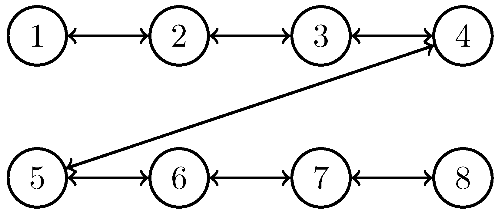
In this section, numerical studies are carried out for a multi-train system with $N=8$ trains. The communication topology is the bidirectional line graph shown in Figure 1. Each train i communicates only with its immediate predecessor $i-1$ and successor $i+1$ for $i=2,\dots ,7$, while train 1 communicates only with train 2 and train 8 communicates only with train 7. All edge weights $a_{ij}$ are set to 1. The train masses are $m_i=6\times {10}^5\mathrm{kg}$ for $i=1,3,5,7$ and $m_i=3.6\times {10}^5\mathrm{kg}$ for $i=2,4,6,8$.

The Davis resistance parameters are listed in

Table 2. Parameters of the high-speed train model.

Parameter	Value	Unit
$c_0$	$1.176\times {10}^{-2}$	N/kg
$c_{v,nom}$	$7.7616\times {10}^{-4}$	N·s/(m·kg)
$c_{a,nom}$	$1.6\times {10}^{-5}$	N·s2/(m2·kg)

. For the stress-test case, the resistance coefficients are generated as

$$\begin{array}{c}\hfill {\theta }_i\left(t\right)={\theta }_{\mathrm{nom}}\left[1+0.38sin(0.55t+0.37i)+0.18sin(1.45t+0.23i)\right],\end{array}$$

(36)

with saturation to keep the coefficients positive. In addition, train 1 experiences a $60\%$ temporary aerodynamic increase during $t\in [75,95]\mathrm{s}$, and train 4 experiences a $45\%$ increase during $t\in [125,145]\mathrm{s}$. The state constraints are $V_i=[0,85]\mathrm{m}/\mathrm{s}$ and $d_{\mathrm{safe}}=500\mathrm{m}$, and the desired adjacent spacing is $|{\overline{r}}_{ij}|=1500\mathrm{m}$. The normalized actuator interval is $U_i=[-1,1]$.

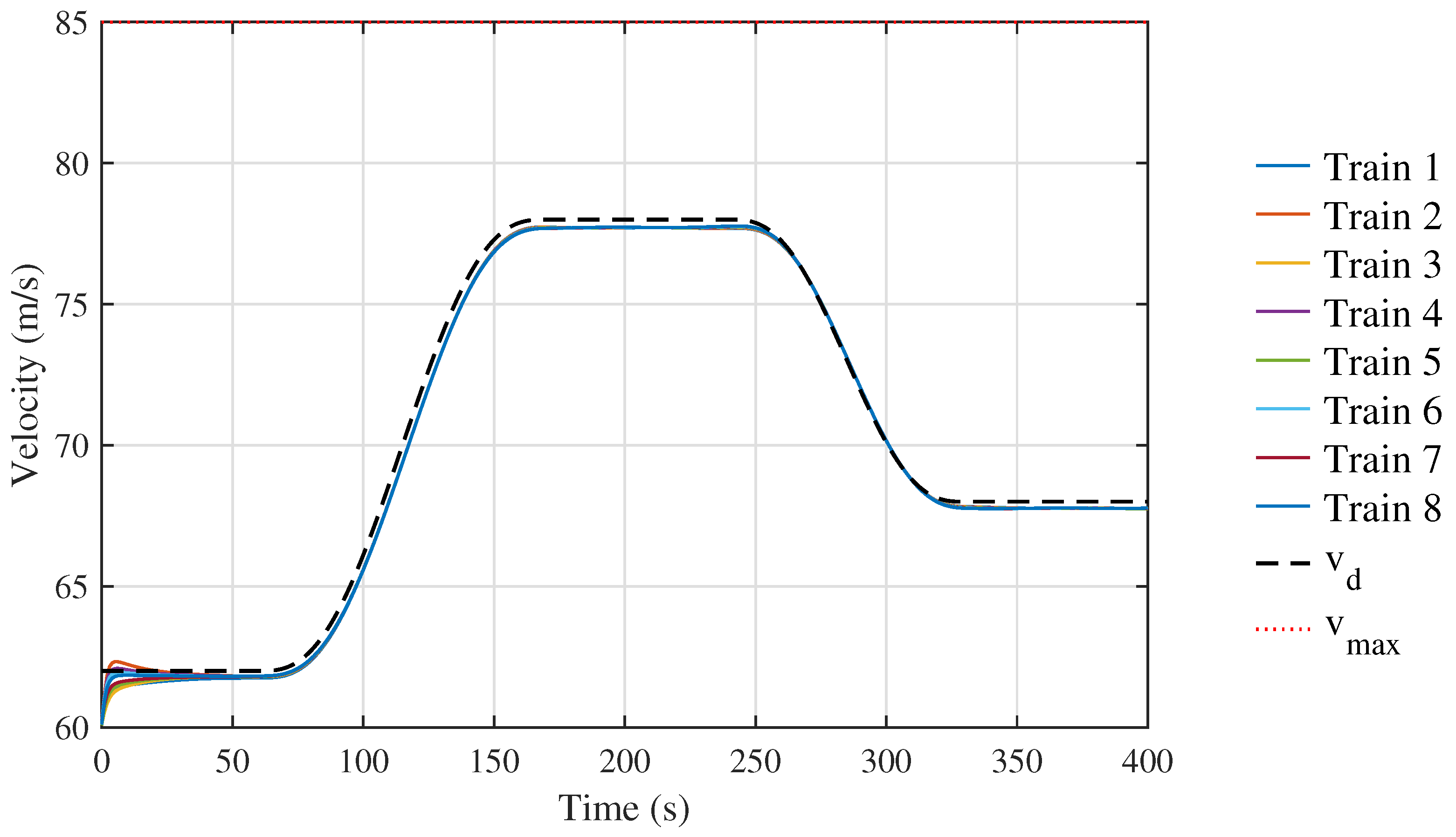
Two simulation cases are considered. Case I is a nominal multi-phase tracking task, where the desired speed starts from $62\mathrm{m}/\mathrm{s}$, increases to $78\mathrm{m}/\mathrm{s}$, and then decreases to $68\mathrm{m}/\mathrm{s}$. Case II is a stress test with faster time-varying resistance and speed operation close to the upper velocity constraint. In Case II, the initial adjacent gaps are 1110–$1530\mathrm{m}$, the initial velocities are approximately 70–$70.95\mathrm{m}/\mathrm{s}$, and the desired speed rises from $70\mathrm{m}/\mathrm{s}$ to $83.2\mathrm{m}/\mathrm{s}$ before decreasing to $72\mathrm{m}/\mathrm{s}$. For this stress case, the feasibility quantities in Assumption 5 were checked using the actual simulation parameters. The resulting margins are ${\delta }_v=0.90\mathrm{m}/{\mathrm{s}}^2$, ${min}_i{\eta }_{s,i}\left(0\right)=0.29\mathrm{m}/\mathrm{s}$, and ${\delta }_s=0.04\mathrm{m}/{\mathrm{s}}^2$, confirming that the initial condition lies in the controlled admissible set and that the saturated actuator has inward-pointing authority at the active constraint boundaries.

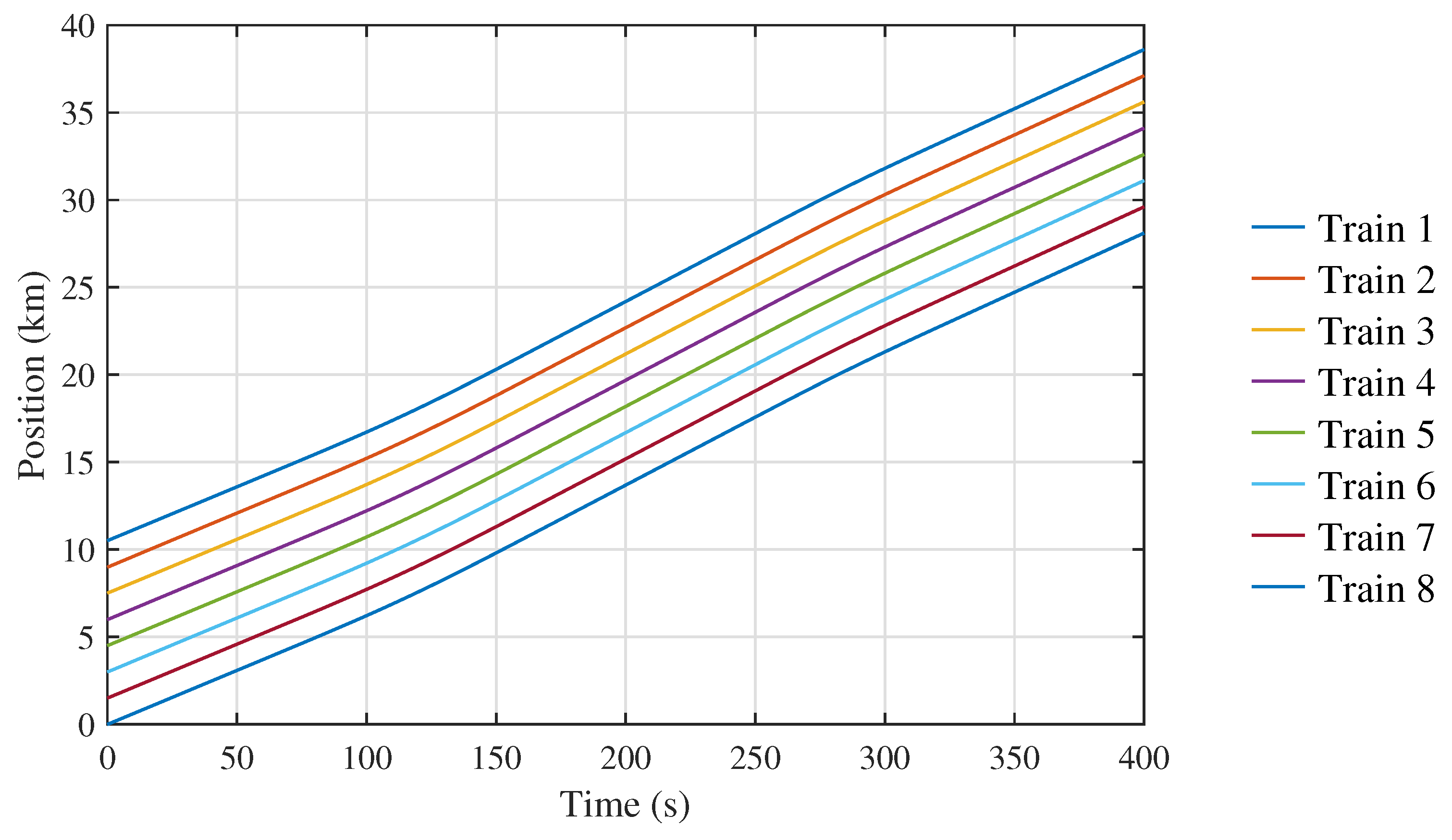
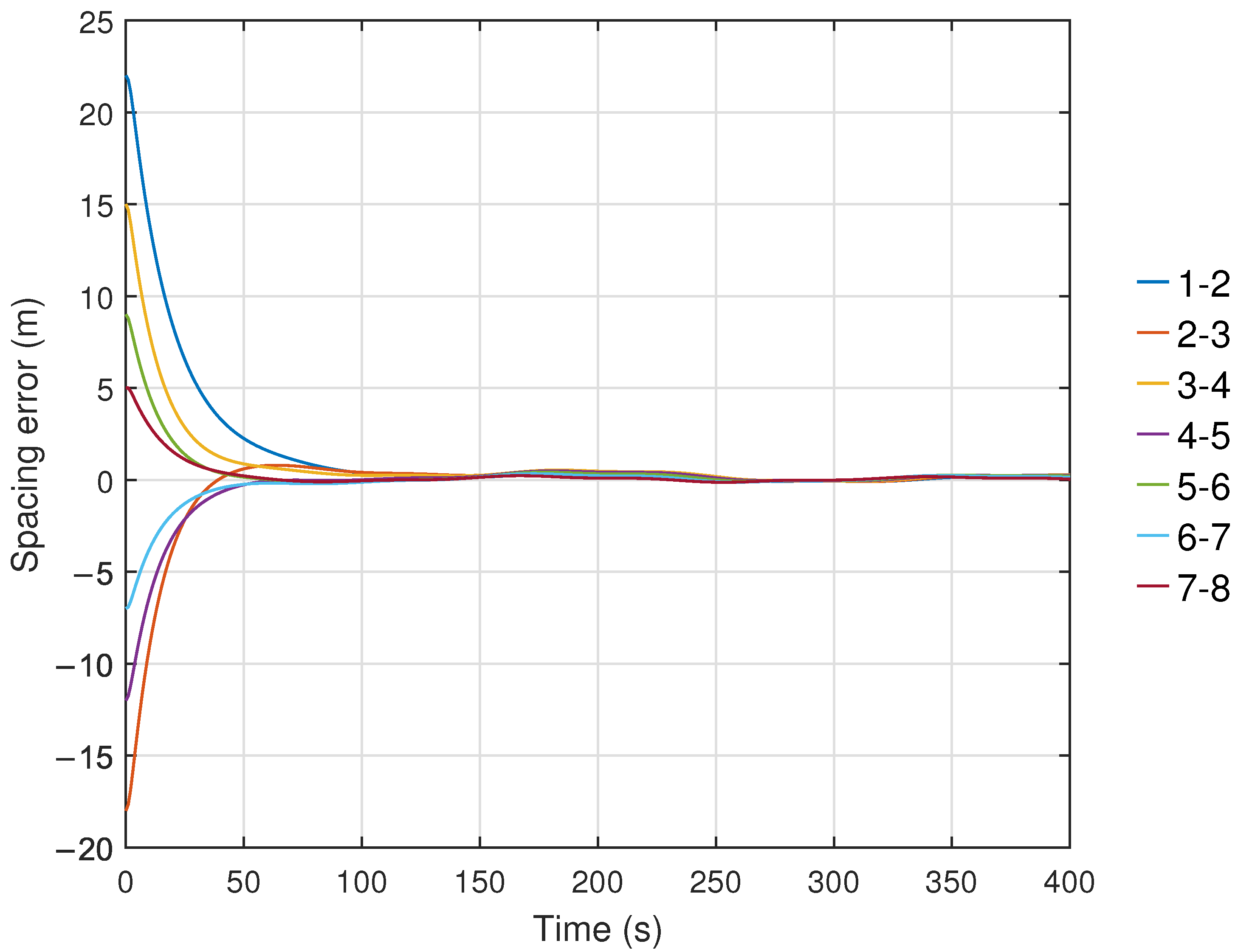
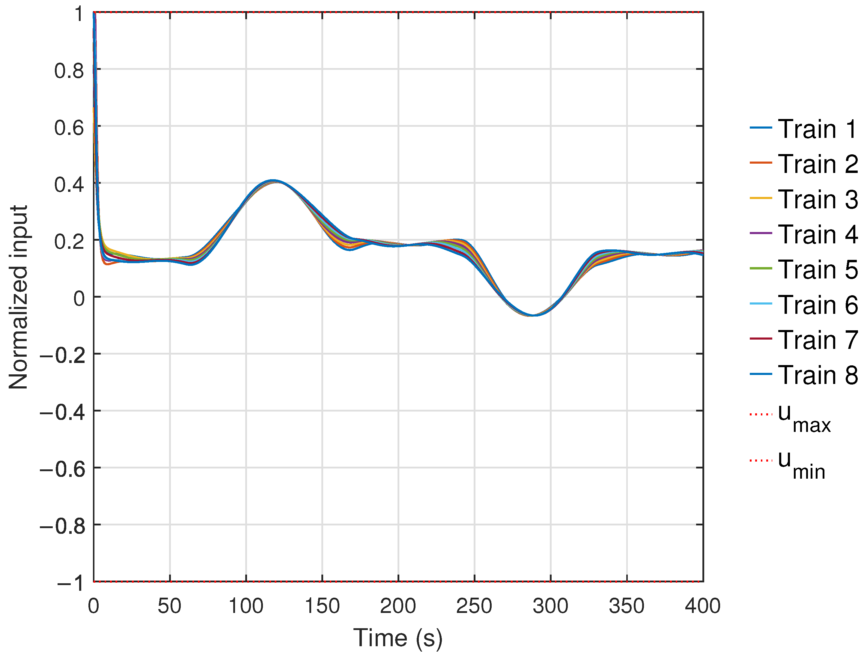
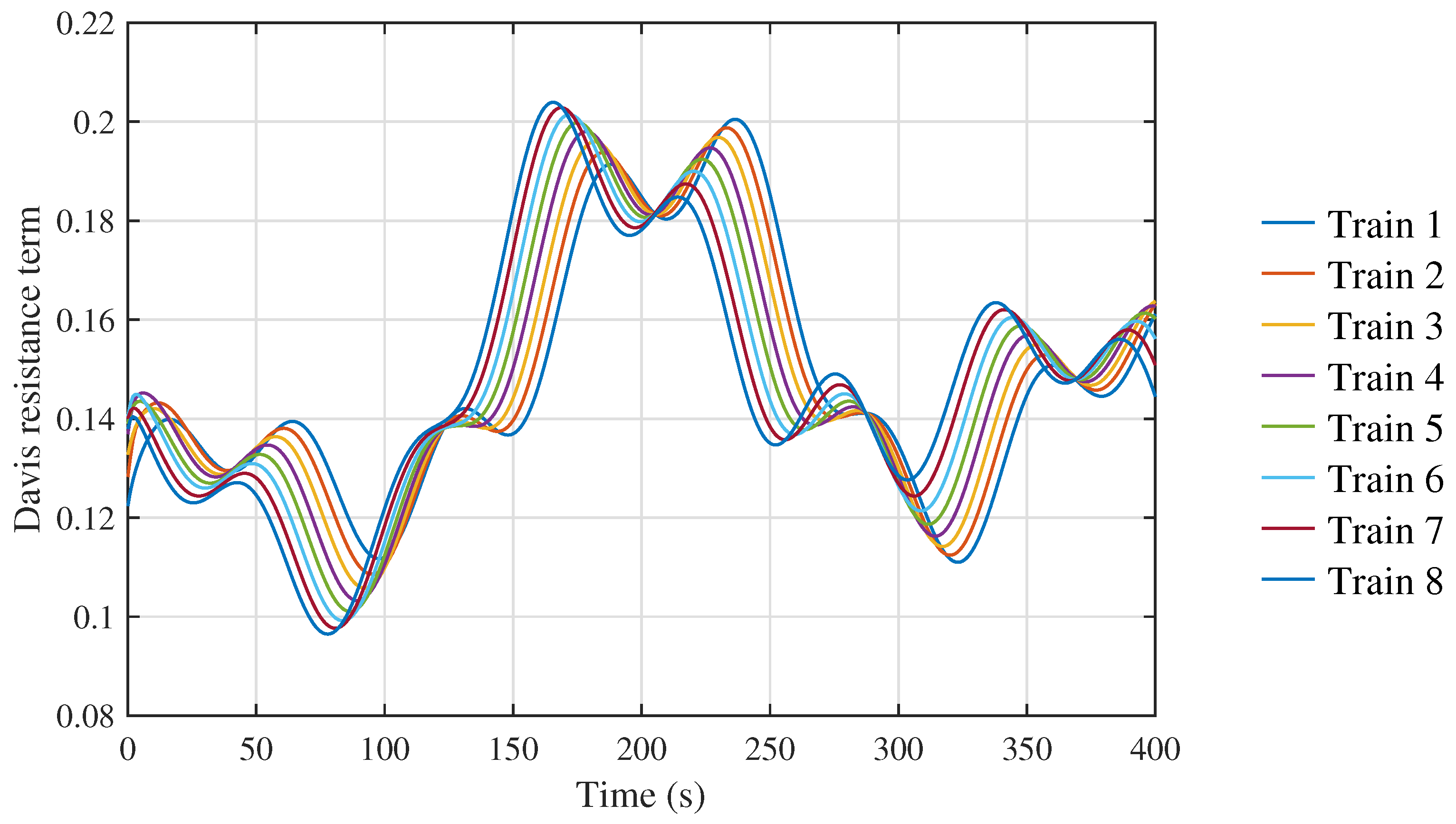
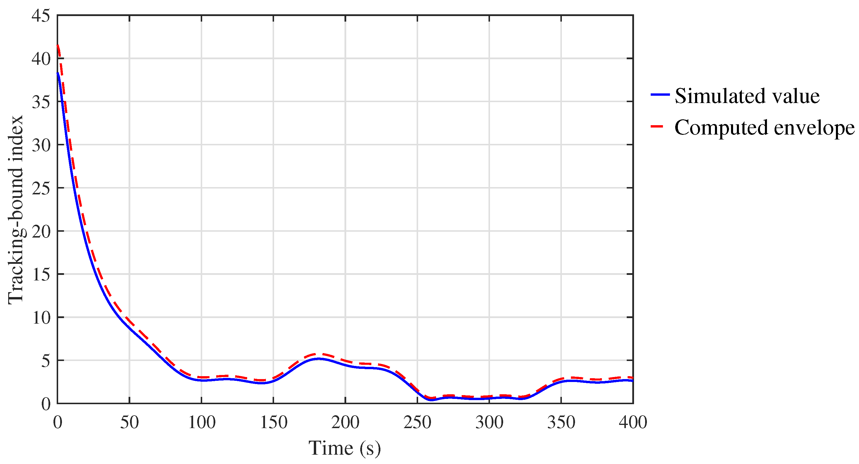
Figure 2, Figure 3, Figure 4, Figure 5 and Figure 6 show the nominal tracking performance. The position trajectories remain ordered, the velocities follow the prescribed multi-phase speed command, and the spacing errors converge from the initial mismatch to a small neighborhood of zero. Figure 5 reports the actual normalized actuator input $u_i\left(t\right)={\mathrm{Sat}}_{U_i}\left[u_{c,i}\left(t\right)\right]$ applied to the train model, rather than the unsaturated raw command $u_{c,i}\left(t\right)$. Thus the plotted signal is the bounded traction/braking command entering the longitudinal dynamics, and it remains within $[-1,1]$. The maximum velocity tracking error is $1.92\mathrm{m}/\mathrm{s}$ and the maximum adjacent-spacing error is $22.0\mathrm{m}$, both below their computed envelopes $2.12\mathrm{m}/\mathrm{s}$ and $24.3\mathrm{m}$, respectively. Figure 7 further confirms the tracking-bound calculation: the maximum simulated tracking norm is $38.34$, while the computed envelope is $41.56$. The maximum command-allocation deviation and resistance bound recorded in the simulation are $0.85$ and $0.20$, respectively.

The original stress test in

Table 3. Quantitative stress-test comparison with modern constrained control benchmarks.

Method	${\mathit{d}}_{min}$ (m)	${\mathit{v}}_{max}$ (m/s)	$max|{\mathit{u}}_{\mathit{i}}|$	Main Observation
Proposed full allocation	$1110.0$	$83.60$	$1.00$	Maintains both spacing and velocity constraints under the stress disturbance.
Distance-only constrained BLF-type benchmark [18]	$1110.0$	$85.57$	$1.00$	Preserves the spacing margin but exceeds the velocity limit, showing that distance-oriented protection alone is insufficient for the coupled stress case.
Velocity/input-constrained benchmark [16]	$1110.0$	$83.60$	$1.00$	Satisfies the speed bound and keeps a large spacing margin in this case, but does not explicitly encode closing-speed spacing safety.
Nominal tracking controller	$1110.0$	$85.57$	$1.00$	Without the full safety allocation, the maximum speed exceeds the prescribed limit.

mainly examines the combined effect of time-varying resistance, velocity protection, and normalized input saturation. Since the minimum gap in that case is still much larger than $d_{\mathrm{safe}}=500\mathrm{m}$, it does not strongly activate the spacing-safety barrier. To directly test the proposed closing-speed-aware spacing barrier, an additional near-boundary diagnostic case is introduced. In this case, the first adjacent gap is initialized as

$$d_{12}\left(0\right)=530.0\mathrm{m},$$

and the follower train is initialized with a positive closing speed of

$$v_2\left(0\right)-v_1\left(0\right)=2.0\mathrm{m}/\mathrm{s}.$$

The remaining train gaps and velocities follow the same stress-test setting, and the same normalized input saturation, time-varying Davis resistance, and controller gains are used. Therefore, the purpose of this additional case is to move the operating point close to the spacing boundary and verify whether the spacing barrier actually affects the applied control input.

The results in

Table 4. Near-boundary spacing-barrier activation diagnostic.

Diagnostic Indicator	Value
Initial adjacent gap, $d_{12}\left(0\right)$	$530.0\mathrm{m}$
Initial closing speed, $v_2\left(0\right)-v_1\left(0\right)$	$2.0\mathrm{m}/\mathrm{s}$
Minimum adjacent gap, $d_{min}$	$529.0\mathrm{m}$
Minimum spacing-safety margin, ${min}_i{\eta }_{s,i}$	$1.00\mathrm{m}/\mathrm{s}$
Spacing allocation active samples	1113
Maximum input difference from constrained baseline	$0.117$

show that the minimum distance remains above the safety distance, with

$$d_{min}=529.0\mathrm{m}>d_{\mathrm{safe}},$$

and the dynamic spacing margin remains positive, with

$$\underset{i}{min}{\eta }_{s,i}=1.00\mathrm{m}/\mathrm{s}.$$

More importantly, the spacing-safety allocation is active for 1113 sampled instants, and the maximum input difference between the full controller and the velocity/input-only constrained baseline reaches $0.117$. These two quantities indicate that the spacing barrier is not passive in this diagnostic case; it contributes directly to the applied control signal when the follower approaches the safety boundary with a nonzero closing speed.

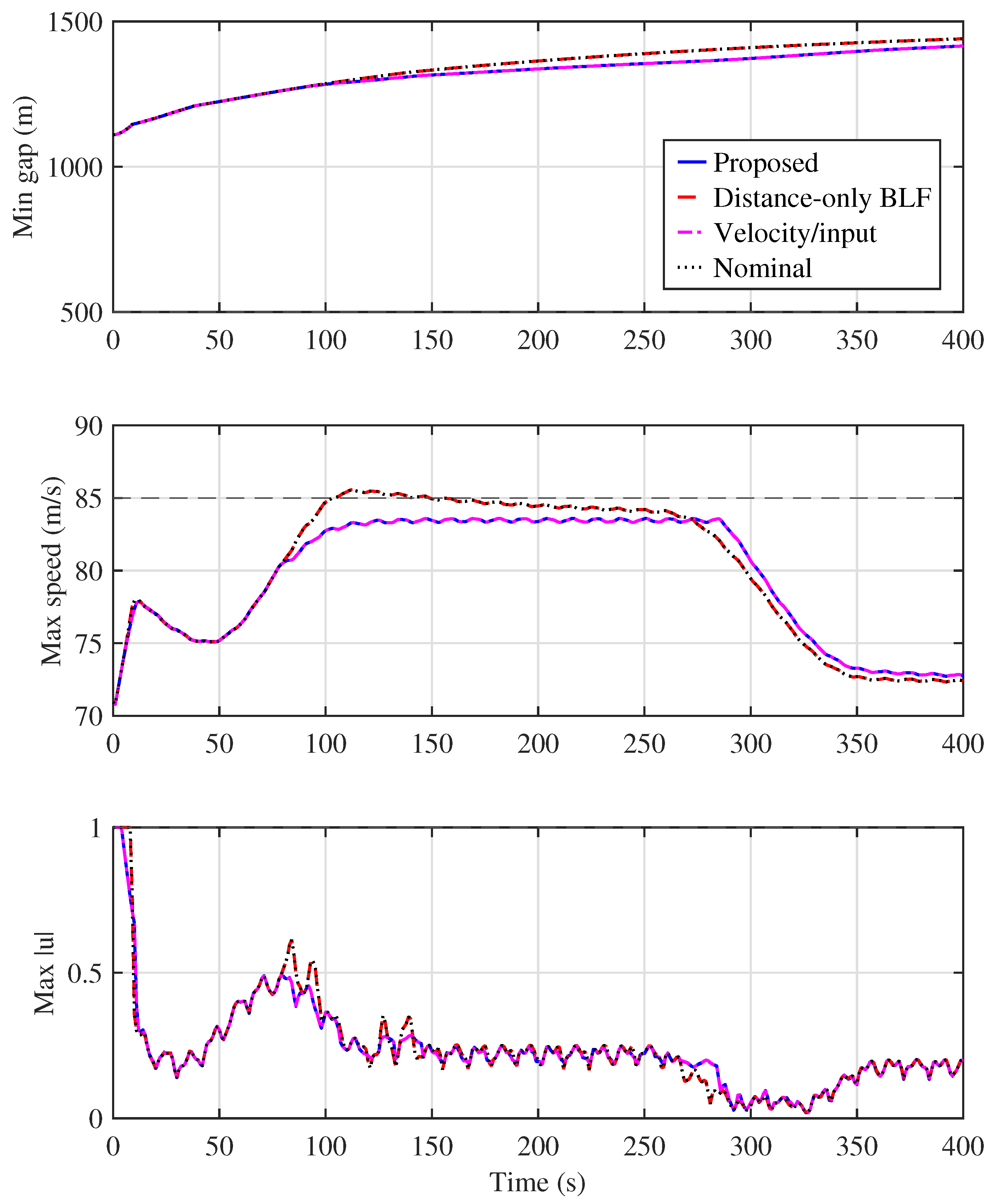
Figure 8 and Table 3 provide the requested comparison with modern constrained control approaches. The distance-only constrained BLF-type benchmark is aligned with the full-state constrained virtual-coupling category represented by [18]. It is constructed in the same simulation framework and under the same plant, time-varying resistance, initial conditions, normalized saturation bounds, and evaluation indices as the proposed controller, but it retains distance-oriented spacing protection instead of the proposed closing-speed-aware integrated safety allocation. This is a structurally matched, literature-aligned benchmark rather than a claim of exact reproduction, because implementation-specific source code and tuning data for [18] are unavailable. The velocity/input-constrained benchmark is aligned with [16] and enforces the speed and actuator bounds without explicitly encoding the closing-speed spacing margin.

All constrained variants keep the minimum spacing above $d_{\mathrm{safe}}=500\mathrm{m}$ for this initial condition, with the smallest recorded gap equal to $1110.0\mathrm{m}$ for the proposed method. The principal difference appears in the velocity constraint: the proposed full allocation limits the maximum speed to $83.60\mathrm{m}/\mathrm{s}$, whereas the distance-only constrained BLF-type benchmark reaches $85.57\mathrm{m}/\mathrm{s}$ and violates the $85\mathrm{m}/\mathrm{s}$ speed bound. The velocity/input-constrained benchmark limits the maximum speed to $83.60\mathrm{m}/\mathrm{s}$ but does not include dynamic closing-speed protection. These results demonstrate the contribution of the proposed coupled spacing–velocity–input design against constrained alternatives, while PID and SMC are retained only as additional familiar engineering references.

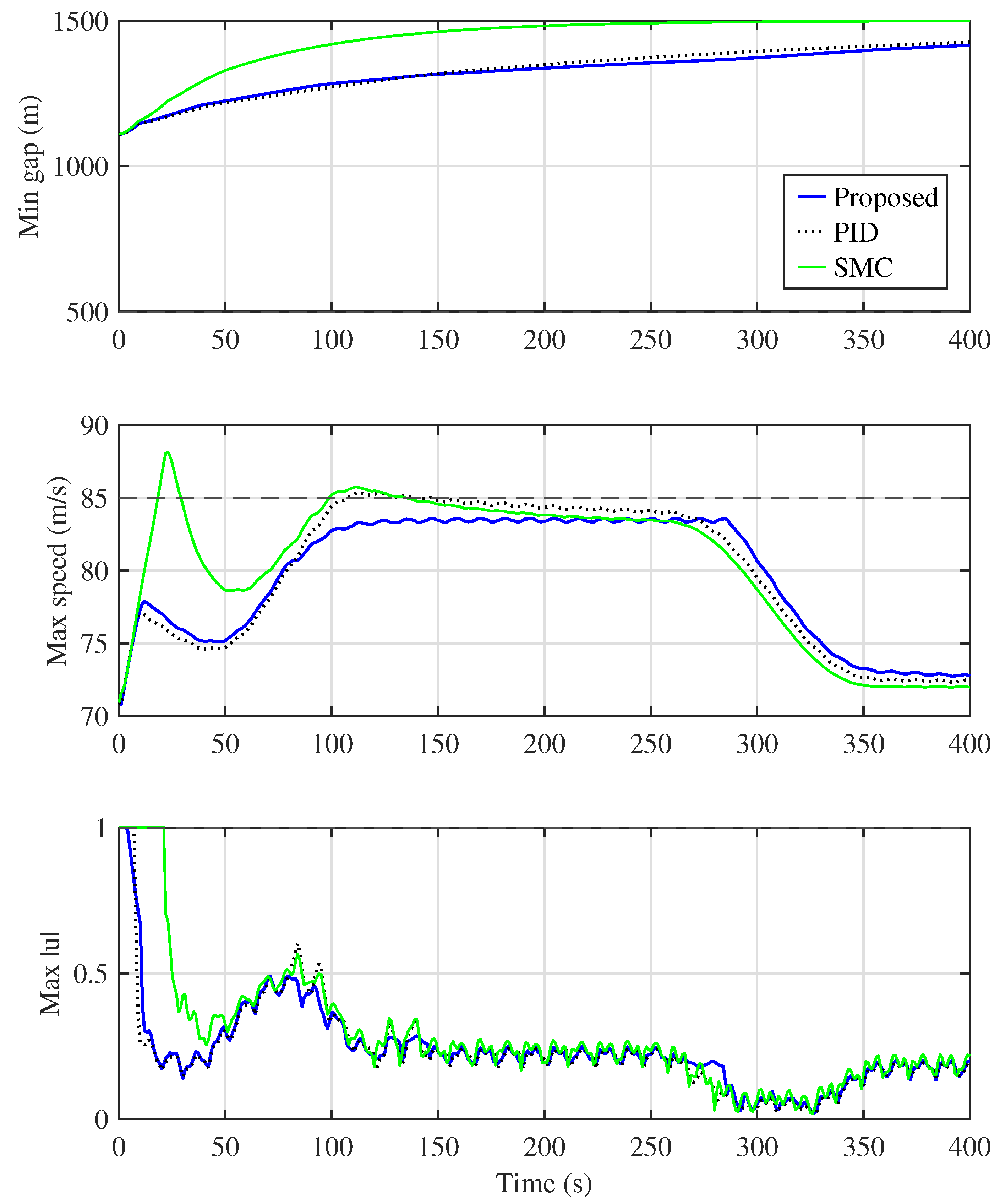
Figure 9 and

Table 5. Quantitative benchmark comparison with PID and SMC controllers under the near-boundary stress-test condition.

Method	${\mathit{E}}_{\mathit{v}}$ (m/s)	${\mathit{E}}_{\mathit{s}}$ (m)	${\mathit{d}}_{min}$ (m)	${\mathit{v}}_{max}$ (m/s)	${\mathit{J}}_{\mathit{u}}$	Main Observation
Proposed method	$1.43$	$146.0$	$1110.0$	$83.60$	$58.6$	Preserves the velocity and spacing constraints under normalized saturation.
PID benchmark	$1.37$	$140.4$	$1110.0$	$85.37$	$57.4$	Gives comparable RMS tracking indices but exceeds the prescribed velocity bound.
SMC benchmark	$2.59$	$82.1$	$1110.0$	$88.17$	$92.5$	Reduces the spacing RMS index but violates the velocity bound and produces the largest input activity.

further compare the proposed controller with PID and SMC benchmarks under the same stress-test condition. The PID benchmark has a similar RMS velocity-tracking index, but its maximum speed reaches $85.37\mathrm{m}/\mathrm{s}$ and therefore violates the velocity constraint. The SMC benchmark improves the spacing RMS index to $82.1\mathrm{m}$, but it reaches $88.17\mathrm{m}/\mathrm{s}$ and produces the largest input activity $J_u=92.5$. In contrast, the proposed method keeps the maximum speed at $83.60\mathrm{m}/\mathrm{s}$ while maintaining the spacing constraint and moderate input activity. Thus, the main advantage of the proposed method is not merely lower nominal RMS error, but simultaneous constraint satisfaction under time-varying resistance and saturated actuation.

Quantitative Parameter Sensitivity and Tuning

To quantify the influence of the main design parameters, a one-factor-at-a-time sensitivity study was performed under the same time-varying-resistance stress profile and normalized saturation interval used above. The barrier gains $(k_{b,v},k_{b,s})$, adaptation gain matrix ${\mathrm{\Gamma }}_i$, anti-windup gain $k_{\xi ,i}$, and $\sigma$-modification coefficient ${\sigma }_i$ were independently multiplied by $0.5$, $1.0$, and $2.0$, while all other parameters and initial conditions were fixed. The nominal values used in this study were

$$(k_{b,v},k_{b,s})=(1.38,0.88),{\mathrm{\Gamma }}_i=diag(2.0\times {10}^{-8},4.0\times {10}^{-12}),k_{\xi ,i}=1.20,{\sigma }_i=0.08.$$

The performance indices are the RMS velocity-tracking error $E_v$, RMS adjacent-spacing error $E_s$, minimum adjacent gap $d_{min}$, maximum velocity $v_{max}$, and total input variation

$$J_u={\displaystyle \sum _{i=1}^n}{\displaystyle \sum _{k=2}^N}|u_i\left(t_k\right)-u_i\left(t_{k-1}\right)|.$$

The maximum normalized input equals $1.0$ in every case and is therefore not repeated in

Table 6. One-factor-at-a-time sensitivity study under the time-varying-resistance stress condition.

Parameter Group	Multiplier	${\mathit{E}}_{\mathit{v}}$ (m/s)	${\mathit{E}}_{\mathit{s}}$ (m)	${\mathit{d}}_{min}$ (m)	${\mathit{v}}_{max}$ (m/s)	${\mathit{J}}_{\mathit{u}}$
Barrier gains $(k_{b,v},k_{b,s})$	$0.5$	1.171	161.32	1110.0	84.09	55.0
	$1.0$	1.305	163.21	1110.0	83.60	56.3
	$2.0$	1.609	165.27	1110.0	82.90	57.7
Adaptation gain ${\mathrm{\Gamma }}_i$	$0.5$	1.316	163.45	1110.0	83.59	56.1
	$1.0$	1.305	163.21	1110.0	83.60	56.3
	$2.0$	1.288	162.76	1110.0	83.62	56.5
Anti-windup gain $k_{\xi ,i}$	$0.5$	1.304	163.25	1110.0	83.60	56.2
	$1.0$	1.305	163.21	1110.0	83.60	56.3
	$2.0$	1.305	163.19	1110.0	83.60	56.3
$\sigma$-modification coefficient ${\sigma }_i$	$0.5$	1.305	163.21	1110.0	83.60	56.3
	$1.0$	1.305	163.21	1110.0	83.60	56.3
	$2.0$	1.305	163.21	1110.0	83.60	56.3

.

All 12 parameter combinations preserve the constraints: $d_{min}=1110.0\mathrm{m}>d_{\mathrm{safe}}=500\mathrm{m}$, $v_{max}<85\mathrm{m}/\mathrm{s}$, and $max|u_i|=1$. The barrier gains have the strongest influence on the safety–performance tradeoff. Increasing their multiplier from $0.5$ to $2.0$ reduces $v_{max}$ from $84.09$ to $82.90\mathrm{m}/\mathrm{s}$, but increases $E_v$ from $1.171$ to $1.609\mathrm{m}/\mathrm{s}$ and $J_u$ from $55.0$ to $57.7$. Thus, larger barrier gains increase the velocity-bound reserve at the cost of tracking accuracy and input activity. The unchanged minimum gap is consistent with the large initial spacing reserve in this stress case; the separate near-boundary case in Table 4 is used to verify activation of the spacing barrier when that reserve is small.

Increasing ${\mathrm{\Gamma }}_i$ from $0.5$ to $2.0$ times its nominal value slightly reduces $E_v$ from $1.316$ to $1.288\mathrm{m}/\mathrm{s}$ and $E_s$ from $163.45$ to $162.76\mathrm{m}$, while increasing $J_u$ from $56.1$ to $56.5$. The anti-windup-gain variations change the reported external indices by less than approximately $0.1\%$, because the saturation intervals are limited and the auxiliary state decays rapidly for all three positive gains. Similarly, varying ${\sigma }_i$ produces no visible change at the reported precision. This does not make the leakage term unnecessary: its main role is to suppress long-term parameter drift and preserve robustness during weakly exciting cruising, whereas its direct effect on finite-horizon tracking is small when the resistance remains bounded and the estimates stay close to the nominal values. These numerical trends apply to the tested $0.5$–$2.0$ range; excessively small or large gains can invalidate the dissipation inequalities, amplify estimate oscillations, or increase actuator activity and are not covered by this study.

The nominal gains were selected in two stages. The interior tracking and coupling gains were first chosen according to the local string-stability guideline. The barrier gains were then increased until the desired velocity reserve was obtained without excessive input variation, after which $k_{\xi ,i}$, ${\mathrm{\Gamma }}_i$, and ${\sigma }_i$ were adjusted to obtain bounded transient compensation and parameter estimates. Table 6 makes these tuning tradeoffs quantitative rather than relying only on qualitative guidance.

4. Discussion

The contribution of this study should be interpreted at the constrained virtual-coupling level rather than as a separate use of existing BLF, CBF, adaptive-control, or anti-windup tools. The first contribution is a unified safety-tracking formulation for high-density train operation, where continuously varying speed commands, velocity limits, spacing safety, normalized saturation, and time-varying Davis resistance interact in real time. The second contribution is the integration of a closing-speed-aware spacing margin into a saturated adaptive cooperative controller. Although the safety variable is related to high-relative-degree CBF ideas, it is not used as an external safety filter; it is part of the closed-loop adaptive control and Lyapunov analysis. The third contribution is the associated verification framework, which combines the proof-order clarification, feasibility-margin interpretation, near-boundary activation diagnostic, and constrained-baseline comparisons.

The revised numerical results support these contributions. The stress-test comparison now includes a literature-aligned distance-only constrained BLF-type benchmark [18] and a velocity/input-constrained benchmark [16], in addition to PID and SMC. The former preserves the distance margin but still violates the velocity constraint under strong resistance variation, whereas the latter enforces the tested speed and input bounds without explicitly protecting the dynamic closing-speed margin. The near-boundary activation case further shows that the proposed spacing term changes the applied input when the follower approaches the safety boundary with nonzero closing speed. Thus, the evidence for the proposed method is based on comparison with constrained alternatives, while the PID and SMC results serve only as familiar engineering references.

The quantitative sensitivity study further identifies the barrier gains as the dominant safety–performance tuning factors in the tested range: increasing them improves the velocity-bound reserve but increases the RMS tracking error and total input variation. The adaptation gain produces a smaller accuracy–activity tradeoff, whereas the anti-windup and $\sigma$-modification gains have limited influence on the reported finite-horizon external indices for the tested stress case. Their principal roles remain saturation-residual dissipation and prevention of long-term parameter drift, respectively.

Point-mass modeling is an established first step in longitudinal train-control research because it preserves the dominant force balance and inter-train kinematics while keeping the control mechanisms and theoretical assumptions transparent. The present evaluation therefore provides meaningful method-level evidence for cooperative tracking, safety constraints, saturation handling, and resistance adaptation. At the same time, it cannot quantify the effects of in-train forces, adhesion loss, actuator lag, suspension and carbody motion, or route-dependent excitation. Validation will consequently proceed in three further stages. First, the controller will be evaluated using a high-fidelity longitudinal train model with distributed masses, coupler/buffer forces, wheel–rail adhesion constraints, and traction/braking dynamics. Second, longitudinal control will be coupled to a multibody vehicle model to evaluate carbody response, suspension interaction, passenger comfort, and actuator-rate demand. Third, the complete virtual-coupling system will be tested in a realistic railway simulator or hardware-in-the-loop platform using measured route, actuator, resistance, and communication characteristics. The nominal, stress-test, near-boundary, and constrained-baseline scenarios used here will be repeated at each stage so that changes in safety margin, tracking error, saturation duration, and input activity can be quantified consistently.

4.1. Measurement, Communication, and Actuation Nonidealities

The theoretical analysis assumes exact position and velocity signals. In practice, odometry, speed sensing, train localization, and inter-train ranging are affected by noise, bias, quantization, and bounded estimation errors. Let the measured states be ${\widehat{x}}_i=x_i+n_{x,i}$ and ${\widehat{v}}_i=v_i+n_{v,i}$, where $|n_{x,i}|\le {\epsilon }_x$ and $|n_{v,i}|\le {\epsilon }_v$. Since the dynamic spacing variable contains both relative position and relative velocity, a robust implementation should tighten the measured safety margins according to

$$\begin{array}{cc}\hfill h_{s,i}^{\mathrm{rob}}& ={\widehat{x}}_{i-1}-{\widehat{x}}_i-d_{\mathrm{safe}}-2{\epsilon }_x,\hfill \\ \hfill {\eta }_{s,i}^{\mathrm{rob}}& ={\widehat{v}}_{i-1}-{\widehat{v}}_i-2{\epsilon }_v+{\alpha }_{s,i}{h}_{s,i}^{\mathrm{rob}}.\hfill \end{array}$$

(37)

Positivity of these tightened quantities accounts for the worst-case relative measurement error. This issue is particularly important for $B_{s,i}=k_{b,s}/{\eta }_{s,i}$, because reciprocal barrier terms can amplify high-frequency measurement noise when the safety margin is small. Consequently, raw measured signals should not be inserted directly into the barrier. A practical implementation requires a state observer or bandwidth-limited filter, together with explicit uncertainty margins. Filtering alone is not sufficient because its phase lag can also reduce the apparent closing speed and delay the safety response.

Communication delay and packet loss affect the same safety channel. Delayed predecessor data can overestimate the current gap or underestimate an increasing closing speed. If the end-to-end delay is bounded by $\overline{\tau }$, a conservative distance allowance can be introduced as

$$\begin{array}{c}\hfill d_{\mathrm{safe}}^{\mathrm{rob}}=d_{\mathrm{safe}}+2{\epsilon }_x+{\overline{v}}_{\mathrm{rel}}\overline{\tau }+{\displaystyle \frac{1}{2}}{\overline{a}}_{\mathrm{rel}}{\overline{\tau }}^2,\end{array}$$

(38)

where ${\overline{v}}_{\mathrm{rel}}$ and ${\overline{a}}_{\mathrm{rel}}$ bound the relative speed and acceleration during the communication age. Time-stamped packets and predictor-based reconstruction can reduce conservatism, but the prediction error must remain inside the tightened margin. During packet loss, zero-order-hold data should be permitted only up to a verified maximum dropout interval. If the packet age exceeds this limit, the cooperative controller should switch to a local safety mode using onboard ranging and emergency-braking logic. Proving invariance with these effects would require a delay-dependent Lyapunov–Krasovskii, sampled-data, or hybrid-system analysis; the delay-free theorem in this paper does not provide such a guarantee.

The actuator model also requires qualification. The simulations use the instantaneous static relation $u_i={\mathrm{Sat}}_{U_i}\left[u_{c,i}\right]$, whereas a traction/braking system has command lag, rate limits, switching logic, dead zones, and possibly adhesion-dependent force loss. A first implementation model is

$$\begin{array}{cccc}\hfill {\dot{u}}_{a,i}& ={sat}_{[-r_u,r_u]}\left({\displaystyle \frac{{\mathrm{Sat}}_{U_i}\left[u_{c,i}\right]-u_{a,i}}{{\tau }_u}}\right),\hfill & \hfill u_i& =u_{a,i},\hfill \end{array}$$

(39)

where ${\tau }_u>0$ and $r_u>0$ are the actuator time constant and rate bound. With this model, the anti-windup residual must be redefined as ${\mathrm{\Delta }}_i=u_{a,i}-u_{c,i}$. More importantly, actuator lag reduces the instantaneous braking authority used in Assumption 5; therefore, ${\delta }_v$ and ${\delta }_s$ must be recomputed using the worst-case actuator state, rate limit, adhesion level, and switching delay. The actuator state must also be included in an augmented barrier–Lyapunov proof.

The present theorem and simulations therefore establish method-level behavior under exact state exchange and static saturation, but they do not claim robustness guarantees for arbitrary sensor noise, measurement bias, communication delay, packet loss, or actuator lag. Future validation will combine observer-based estimation, delay-aware safety-margin tightening, packet-age supervision, and the rate-limited actuator model in high-fidelity simulation and hardware-in-the-loop experiments. The emergency-braking supervisor will remain independent of the cooperative controller so that a communication failure cannot remove the final local safety layer.

4.2. Computational Requirements and Real-Time Feasibility

The distributed structure avoids a central computational bottleneck. Let $d_i=\left|{\mathcal{N}}_i\right|$ be the local graph degree and let p be the adaptive-parameter dimension. Evaluation of the cooperative position and velocity errors requires $\mathcal{O}\left(d_i\right)$ additions and multiplications. The velocity and spacing barrier terms, saturation, and anti-windup update require a fixed number of scalar operations, while the adaptive update requires $\mathcal{O}\left(p\right)$ operations. Thus, the per-train computational cost and storage are

$$\begin{array}{cccc}\hfill {\mathcal{C}}_i& =\mathcal{O}(d_i+p),\hfill & \hfill {\mathcal{M}}_i& =\mathcal{O}(d_i+p).\hfill \end{array}$$

(40)

For the two-coefficient Davis model, $p=2$. In the nearest-neighbor chain used in the simulations, $d_i\le 2$ regardless of the formation length. The computation is therefore constant per train, and all onboard controllers can execute in parallel. No centralized optimization, matrix inversion, prediction horizon, or iterative numerical solver is required.

The communication payload is also fixed per edge. Each packet needs the neighbor position, velocity, and a time stamp; the adaptive parameters are local and need not be broadcast. The continuous adaptive and anti-windup laws can be implemented with fixed-step updates,

$$\begin{array}{cc}\hfill {\widehat{\theta }}_i[k+1]& ={\widehat{\theta }}_i\left[k\right]+T_s{\dot{\widehat{\theta }}}_i\left[k\right],\hfill \\ \hfill {\xi }_i[k+1]& ={\xi }_i\left[k\right]+T_s{\dot{\xi }}_i\left[k\right],\hfill \end{array}$$

(41)

followed by algebraic evaluation of the barrier terms and saturated command. Higher-order integration can be used if required, but it is not structurally necessary. Since no optimization solver is present, the main implementation constraints are deterministic packet age, sampling jitter, numerical precision, and completion of the local update before the next control deadline.

The present numerical simulations establish algorithmic feasibility but are not worst-case execution-time measurements on a certified railway processor. Real-time deployment therefore requires processor-in-the-loop profiling, communication-stack timing tests, finite-precision assessment, and hardware-in-the-loop validation under the selected sampling period.

4.3. Large-Formation Performance and Computational Load

For a larger formation, the distributed controller retains the same local structure because each train uses only its own state and neighboring-train information. However, increasing the number of trains may increase accumulated tracking errors and affect the convergence process and minimum spacing and velocity margins. The eight-train simulations therefore verify the proposed method only for the tested formation, and additional simulations are required to confirm its dynamic performance for substantially larger formations.

For the nearest-neighbor chain, each train communicates with at most two neighbors. With the two-parameter Davis model, the computational, storage, and communication burden remains $\mathcal{O}\left(1\right)$ per train, while the total burden grows as $\mathcal{O}\left(n\right)$. The controller therefore has a scalable computational structure for large sparse formations, whereas its large-formation control performance still requires quantitative evaluation.

5. Conclusions

This paper has contributed three field-level advances to constrained cooperative train control. First, a unified virtual-coupling safety-tracking problem was formulated for continuously varying speed commands, velocity and spacing constraints, normalized input saturation, and time-varying Davis resistance coefficients. Second, a closing-speed-aware dynamic spacing mechanism was embedded into a saturated robust adaptive controller, so that the relative-degree-two nature of collision avoidance is handled together with anti-windup compensation and resistance adaptation rather than by a distance-only barrier or an external safety filter. Third, a corresponding certification and validation framework was developed, including barrier-storage invariance, Lyapunov UUB analysis, feasibility-margin interpretation, near-boundary activation testing, and constrained-baseline comparisons. The theoretical novelty is the invariance-before-boundedness proof architecture for the coupled saturated closed-loop dynamics, rather than the isolated use of any one established control tool.

The revised simulations show why these contributions matter for virtual-coupling operation. The proposed method preserves both spacing and velocity constraints under normalized input saturation, whereas the literature-aligned distance-only constrained BLF-type benchmark [18] and the nominal variant exceed the prescribed velocity limit in the stress test. The velocity/input-constrained benchmark [16] satisfies the tested speed bound but does not encode the proposed dynamic closing-speed margin. The near-boundary diagnostic confirms that the closing-speed-aware spacing term is active when a follower approaches the safety boundary, and the PID/SMC results provide supplementary engineering references. Therefore, the main outcome is a constraint-aware cooperative control framework whose advantage is evaluated against modern constrained alternatives as well as conventional controllers.

The sensitivity sweep confirms constraint satisfaction over the tested gain range from $0.5$ to $2.0$ times nominal. The barrier gains govern the clearest tradeoff between velocity reserve, tracking accuracy, and input activity, while the adaptation, anti-windup, and $\sigma$-modification gains have smaller effects on the reported finite-horizon external indices.

The point-mass simulations constitute the first stage of the validation process. Because this model retains the essential longitudinal force balance, running resistance, actuator saturation, and inter-train kinematics, it provides an appropriate basis for demonstrating the proposed method and verifying the theoretical results. For the nearest-neighbor chain, the local computation remains constant per train and the total burden grows linearly with the formation size. However, the eight-train results do not establish unchanged dynamic performance for a substantially larger formation, which must be assessed through additional scale simulations. The next validation stages will use high-fidelity longitudinal dynamics, multibody or co-simulation models, and a realistic railway simulator or hardware-in-the-loop platform. They will explicitly include coupler/buffer forces, wheel–rail adhesion, traction/braking dynamics, suspension and carbody response, route data, sensor noise, localization uncertainty, actuator bandwidth, communication delay, and packet loss. Additional theoretical work is required to establish controlled invariance with observer errors, delayed or intermittent neighbor information, switching topology, and rate-limited actuator states.

References

1. Howlett, P.; Pudney, P.; Vu, X. Local energy minimization in optimal train control. Automatica 2009, 45, 2692–2698. [Google Scholar] [CrossRef] [Scilit]
2. Huang, Y.; Fang, W.; Chen, Z.; Li, Y.; Yang, C. Flocking of multiagent systems with nonuniform and nonconvex input constraints. IEEE Trans. Autom. Control 2023, 68, 4329–4335. [Google Scholar]
3. Liu, X.; Xun, J.; Ning, B.; Wang, C. Braking process identification of high-speed trains for automatic train stop control. ISA Trans. 2021, 111, 171–179. [Google Scholar] [CrossRef] [Scilit] [PubMed]
4. Huang, Y.; Duan, M.; Mo, L. Multiagent containment control with nonconvex states constraints, nonuniform time delays, and switching directed networks. IEEE Trans. Neural Netw. Learn. Syst. 2019, 31, 5021–5028. [Google Scholar] [CrossRef] [Scilit]
5. Zhuan, X.; Xia, X. Speed regulation with measured output feedback in the control of heavy haul trains. Automatica 2008, 44, 242–247. [Google Scholar] [CrossRef] [Scilit]
6. Yang, X.; Yang, C.; Yang, C.; Peng, T.; Chen, Z.; Wu, Z.; Gui, W. Transient fault diagnosis for traction control system based on optimal fractional-order method. ISA Trans. 2020, 102, 365–375. [Google Scholar] [CrossRef] [Scilit] [PubMed]
7. Li, S.; Yang, L.; Gao, Z. Coordinated cruise control for high-speed train movements based on a multi-agent model. Transp. Res. Part C Emerg. Technol. 2015, 56, 281–292. [Google Scholar] [CrossRef] [Scilit]
8. Zhao, Y.; Wang, T.; Karemi, H. Distributed cruise control of high-speed trains. J. Franklin Inst. 2017, 354, 6044–6061. [Google Scholar] [CrossRef] [Scilit]
9. Tang, H.; Wang, Q.; Feng, X. Robust stochastic control for high-speed trains with nonlinearity, parametric uncertainty, and multiple time-varying delays. IEEE Trans. Intell. Transp. Syst. 2018, 19, 1027–1040. [Google Scholar] [CrossRef] [Scilit]
10. Bai, W.; Lin, Z.; Dong, H.; Ning, B. Distributed cooperative cruise control of multiple high-speed trains under a state-dependent information transmission topology. IEEE Trans. Intell. Transp. Syst. 2019, 20, 2750–2763. [Google Scholar] [CrossRef]
11. Li, S.; Yang, L.; Gao, Z. Distributed optimal control for multiple high-speed train movement: An alternating direction method of multipliers. Automatica 2020, 112, 108646. [Google Scholar] [CrossRef] [Scilit]
12. Wang, X.; Zhu, L.; Wang, H.; Tang, T.; Li, K. Robust distributed cruise control of multiple high-speed trains based on disturbance observer. IEEE Trans. Intell. Transp. Syst. 2021, 22, 267–279. [Google Scholar] [CrossRef] [Scilit]
13. Li, S.; Yang, L.; Gao, Z. Adaptive coordinated control of multiple high-speed trains with input saturation. Nonlinear Dyn. 2016, 83, 2157–2169. [Google Scholar]
14. Huang, Y.; Li, Y. Distributed constrained cooperative control of discrete-time high-speed train systems. In Proceedings of the 2018 International Conference on Intelligent Rail Transportation (ICIRT), Singapore, 12–14 December 2018. [Google Scholar]
15. Huang, Y.; Su, S.; Hou, H.; Li, Y. Cooperative control of high-speed train systems with velocity constraints and parameter uncertainties. Proc. Chin. Intell. Syst. Conf. 2019, 592, 716–723. [Google Scholar] [CrossRef] [Scilit]
16. Lin, P.; Huang, Y.; Zhang, Q.; Yuan, Z. Distributed velocity and input constrained tracking control of high-speed train systems. IEEE Trans. Syst. Man. Cybern. Syst. 2021, 51, 7882–7888. [Google Scholar] [CrossRef] [Scilit]
17. Lin, P.; Tian, Y.; Gui, G.; Yang, C. Cooperative control for multiple train systems: Self-adjusting zones, collision avoidance and constraints. Automatica 2022, 144, 110470. [Google Scholar] [CrossRef] [Scilit]
18. Zhu, L.; Huang, D.; Li, X.; Wang, Q. Cooperative operation control of virtual coupling high-speed trains with input saturation and full-state constraints. IEEE Trans. Autom. Sci. Eng. 2024, 21, 3497–3510. [Google Scholar] [CrossRef] [Scilit]
19. Wang, Q.; Wang, X.; Guo, Y.; Ding, J.; Sun, P.; Feng, X. Robust adaptive iterative learning control for multitrain system with actuator saturation and state constraints. IEEE Trans. Syst. Man. Cybern. Syst. 2025, 55, 6325–6337. [Google Scholar] [CrossRef] [Scilit]
20. Su, S.; Wang, D.; Cao, Y.; Zhou, Y.; Tang, T. Adaptive fault-tolerant fixed-time cruise control for virtually coupled train set. Transp. Res. Part C Emerg. Technol. 2023, 156, 104348. [Google Scholar] [CrossRef] [Scilit]
21. Jin, L.; Qiu, N.; Tian, D.; Zhang, Q.; Huang, K.; Xiao, F. MPC-based path tracking strategy for 4WID&4WIS vehicles using B-spline approximation and state-dependent reference. Control Eng. Pract. 2025, 165, 106546. [Google Scholar] [CrossRef] [Scilit]
22. Ren, Y.; Wang, F.; Shen, T.; Zhao, M.; Zhang, Q.; Yin, G. Hierarchical robust spacing and speed control against chassis actuation perturbations and unknown disturbances. IEEE Trans. Syst. Man. Cybern. Syst. 2026, 56, 2538–2552. [Google Scholar] [CrossRef] [Scilit]
23. Hasarinda, R.; Tharuminda, T.; Palitharathna, K.; Edirisinghe, S. Traffic collision avoidance with vehicular edge computing. In Proceedings of the 2023 3rd International Conference on Advanced Research in Computing (ICARC), Belihuloya, Sri Lanka, 23–24 February 2023; pp. 316–321. [Google Scholar]
24. Ames, A.D.; Xu, X.; Grizzle, J.W.; Tabuada, P. Control barrier function based quadratic programs for safety critical systems. IEEE Trans. Autom. Control 2017, 62, 3861–3876. [Google Scholar] [CrossRef] [Scilit]
25. Nguyen, Q.; Sreenath, K. Exponential control barrier functions for enforcing high relative-degree safety-critical constraints. In Proceedings of the 2016 American Control Conference (ACC), Boston, MA, USA, 6–8 July 2016; pp. 322–328. [Google Scholar]
26. Xiao, W.; Belta, C. Control barrier functions for systems with high relative degree. In Proceedings of the 2019 IEEE 58th Conference on Decision and Control (CDC), Nice, France, 11–13 December 2019; pp. 474–479. [Google Scholar]
27. Huang, Y.; Zhu, Y.; Chen, Z.; Zhang, Z.; Huang, T. A second-order inertial edge-flow competition model for constrained resource competition: Conservation, KKT equilibria, and bounded dominant concentration. Acta Autom. Sci. 2026. [Google Scholar] [CrossRef]
28. Godsil, C.; Royle, G. Algebraic Graph Theory; Springer: New York, NY, USA, 2001. [Google Scholar]
29. Davis, W. The tractive resistance of electric locomotives and cars. Gen. Electr. Rev. 1926, 29, 685–707. [Google Scholar]
30. Khalil, H.K. Nonlinear Systems; Prentice Hall: Upper Saddle River, NJ, USA, 2002. [Google Scholar]
Figure 1. Schematic diagram of the bidirectional line communication graph for N = 8 trains.
Machines 14 00828 g001
Figure 2. Position trajectories in the nominal tracking case. All trains keep their order and move cooperatively with the prescribed formation spacing.
Machines 14 00828 g002
Figure 3. Velocity tracking in the nominal case. The train velocities are compared with the desired profile v d ( t ) and the upper velocity constraint v ¯ i = 85 m / s .
Machines 14 00828 g003
Figure 4. Adjacentspacing errors x i 1 ( t ) x i ( t ) r ¯ i 1 , i in the nominal case. The maximum initial spacing error is 22.0 m , and all spacing errors converge to a small neighborhood of zero.
Machines 14 00828 g004
Figure 5. Normalized control inputs in the nominal case. The input signals remain inside the saturation interval [ 1 , 1 ] .
Machines 14 00828 g005
Figure 6. Time-varying Davis resistance terms in the nominal case. The plot shows the bounded resistance perturbations handled by the robust adaptive design.
Machines 14 00828 g006
Figure 7. Tracking-bound verification. The simulated tracking norm remains below the computed envelope, with maximum values 38.34 and 41.56 , respectively.
Machines 14 00828 g007
Figure 8. Stress-test comparison under time-varying resistance and normalized saturation. The proposed full constraint allocation is compared with a literature-aligned distance-only constrained BLF-type benchmark [18], a velocity/input-constrained benchmark [16], and a nominal tracking variant.
Machines 14 00828 g008
Figure 9. Benchmark comparison under the same near-boundary stress-test condition. The proposed method is compared with a PID controller and a sliding-mode controller with a boundary-layer function.
Machines 14 00828 g009