Research on the Formation Mechanism of Vortices and Key Parameter Regulation in the Electro-Hydraulic Thruster

Abstract

The brake–release stability of electro-hydraulic thrusters (EHTs) significantly affects the safety of hydraulic braking systems, especially under low-temperature conditions with varying fluid viscosity. Most existing studies have focused on macroscopic braking characteristics, while the internal flow field variation and vortex evolution mechanism during the brake–release process remain insufficiently explored. In this work, transient CFD simulations are conducted to investigate vortex formation rules and flow field characteristics inside an EHT. Three typical vortex structures denoted as α, β, and γ are identified, and the independent and coupling influences of fluid dynamic viscosity and motor speed on vortex intensity and piston-bottom pressure are quantitatively analyzed. The results show that vortices α and β trigger flow disorder and additional hydraulic energy loss, while vortex γ optimizes flow uniformity and assists piston extension. Higher fluid viscosity exacerbates vortex development and pressure fluctuation, while increasing motor speed accelerates transient flow field evolution. This study clarifies the internal flow mechanism of EHT brake–release behavior and provides reliable parametric guidance for optimizing the low-temperature performance of electro-hydraulic braking systems.

1. Introduction

An electro-hydraulic brake (EHB) is a common industrial brake device, which is widely used in hoisting machinery, wind power equipment, and sluice brake systems due to its simple structure, low cost, energy efficiency, low noise, and convenient maintenance [1]. EHB realizes braking and releases the brake through its core component, the electro-hydraulic thruster (EHT), and its braking characteristics are closely related to the fluid flow state in the EHT. Under the working condition of low working temperature in cold regions in China, the EHB has such problems as insufficient release torque and long release time, which prevents the braking system from releasing normally [2], which seriously affects the safety and reliability of the brake system.

This problem has drawn considerable attention from domestic and foreign experts and scholars. For rotating hydraulic machinery equipped with impellers and guide vanes, existing numerical investigations have focused on vortex distribution, energy dissipation, and flow field evolution, and the reliability of simulated results is closely associated with mesh quality and turbulence model selection [3]. Jiang et al. [4] analyzed the mechanism of thrust generation of EHT by using fluid dynamics theory and studied its output thrust and braking characteristics. Zhao [5] established the unsteady energy equation of friction pair fluid via an integral method with the cooling hydraulic oil in the clearance of wet brake friction pair as the research object and obtained the three-dimensional temperature and heat flux explicit analytical expressions that can meet the axial and radial boundary conditions at the same time. Han et al. [6,7,8] developed an adaptive slip-mode hydraulic controller based on a hydraulic pressure estimator for the nonlinear and uncertain problems in a sensorless EHB system. Lignon et al. [9,10] analyzed the stability and sensitivity of EHB by establishing a mode coupling mechanism and a relevant dynamic model. Bai and Lv [11] simulated the velocity, pressure, viscosity, and shear stress distribution of the MR fluid flow field in the brake under different disk structures and obtained the variation law of braking torque with the structure and the magnetic field strength. Liu et al. [12] analyzed the velocity distribution of the flow field in the cylindrical MR brake at different braking speeds and magnetic field strengths and obtained the braking torque under the above conditions by using the integral method. Gu et al. [13,14] proposed an indirect method for measuring dynamic braking torque based on the deceleration method and verified the effectiveness of the method through experimental tests. Shen [15] designed a control scheme combining fuzzy control and variable frequency speed regulation technology for an electric hydraulic push rod brake and established an open loop control system of fuzzy brake controller. Wang et al. [16] derived the total transmission ratio of the entire brake system and the lever ratio of the brake mechanism for the commonly used electric hydraulic drum brake. Junior et al. [17] explored the influence of operating parameters such as brake pressure, friction coefficient, and wear on the dynamic stability of the brake system by summarizing the application of complex eigenvalue in the brake system. The above-mentioned studies mainly concentrate on the braking characteristics of the EHB during braking, while there are fewer studies on the braking characteristics of its release process.

In addition, the braking characteristics of EHB are closely related to the fluid flow state in the EHT, especially its internal vortex evolution characteristics. Rafiee and Sadeghiazad [18,19,20] established a computational fluid dynamics (CFD) model based on the experimental model by using the k-epsilon 3D steady state compressible model. Meanwhile, they studied the influence of swirl chamber radius change on the vortex tube performance under various R values and determined the optimal radius of the vortex chamber. Chereparov et al. [21] proposed a Monte Carlo method to simulate fluid flow along a real wall and established a random vortex method using reflection and perturbation techniques to realize multiple Monte Carlo simulations of wall flow. To address the scale-effect issue of tip vortex flow field and initial tip vortex cavitation number, Pu et al. [22,23] simulated the tip vortex flow field velocity of 3D hydrofoil by using the large eddy simulation (LES) turbulence model and proposed a method to calculate the initial tip vortex cavitation number by using the bubble static equilibrium equation. Berestova and Prosvuryakov [24] proposed an accurate solution of the Oberbeck–Boussinesq equation for describing the steady Benard–Rayleigh convection in an infinitely extended horizontal layer. Cao et al. [25,26] numerically studied the influence of Reynolds number (Re) on the mixing process of two-layer density laminar fluid induced by the interaction between the vortex ring and the density interface using an improved vortex-in-cell method. In practical engineering, low-temperature environments will significantly change the physical properties of hydraulic media. The viscosity of hydraulic fluid rises sharply at sub-zero temperatures, which further affects the flow resistance, pressure response, and overall working performance of hydraulic systems [27,28]. Relevant studies have also investigated the viscosity–temperature characteristics of different hydraulic oils and evaluated their performance in low-temperature applications [29]. The above research on vortex characteristics lays a foundation for the research on the fluid vortex characteristics of EHT in this paper.

Taking the EHT as the research object, the formation mechanism and characteristics of vortex in the process of releasing brake are deeply studied in this paper. Compared with existing studies, this work offers clear innovations and addresses key research gaps. Firstly, most of the available literature mainly focuses on the overall braking performance of EHT devices, ignoring microscale flow field evolution and vortex structural variations during the brake–release stage. This study innovatively identifies three typical internal vortex structures and systematically classifies their functional characteristics and working mechanisms. Secondly, traditional parametric studies seldom consider the low-temperature viscosity variation of hydraulic oil and its coupling effect with motor operating speed. This work quantitatively reveals the effects of the two key engineering parameters on vortex intensity distribution and piston pressure response. Thirdly, a quantitative evaluation system for vortex-induced energy loss and flow stability is established, which compensates for the deficiency of qualitative vortex characteristic analysis in previous studies. The research findings provide targeted theoretical support and mechanical insights for the structural optimization and parameter matching of EHTs applied in low-temperature environments.

2. EHB

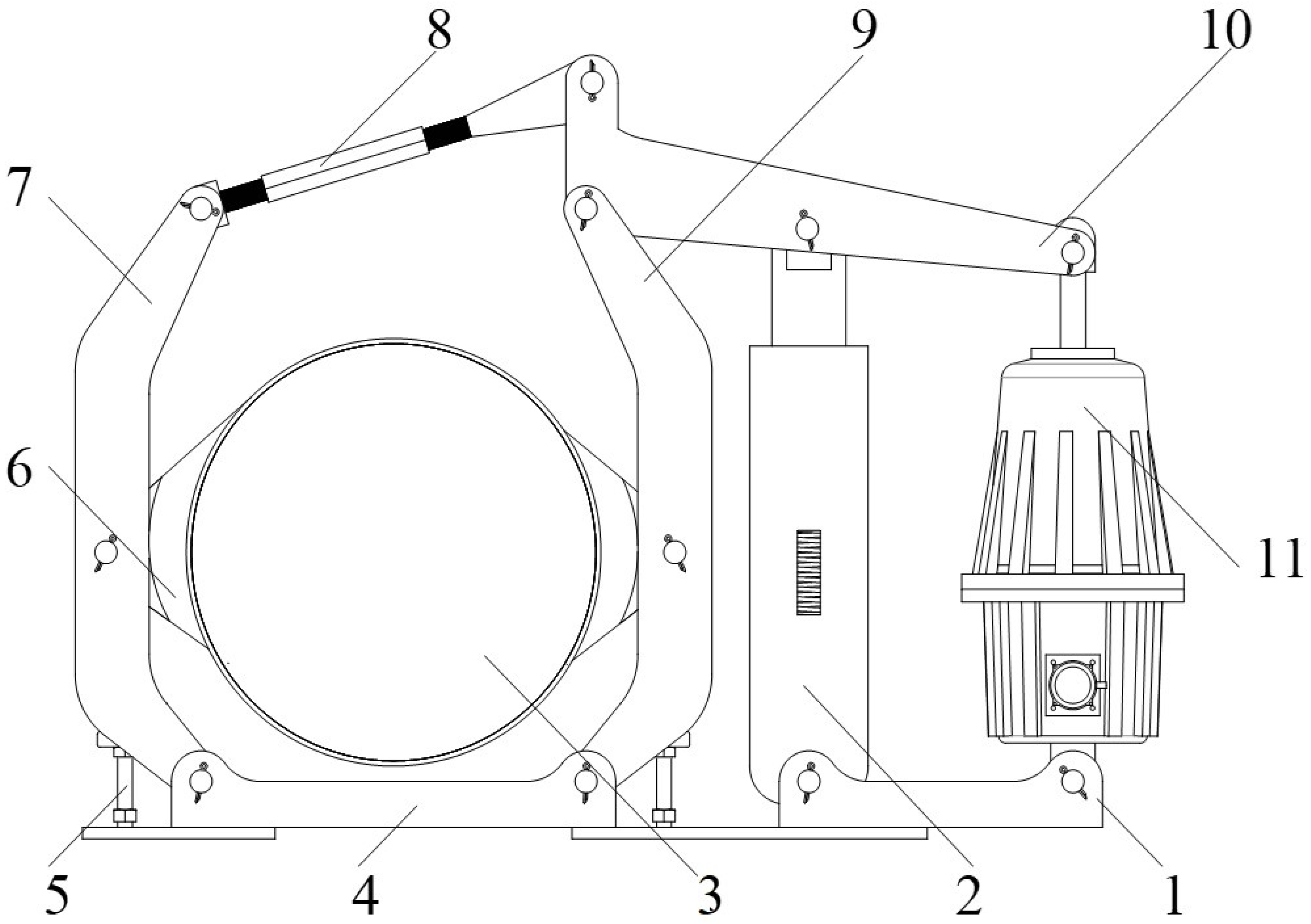
The studied EHB is applied to the brake process and release process of the gate-lifting fixed winch hoist, and its two-dimensional structural model is shown in Figure 1. It is mainly composed of the EHT, spring assembly, retractable threaded rod, transmission plate, brake drum, left and right supporting bolts, and left and right brake arms and base. The EHT mainly includes shell, motor, impeller, and piston assembly. The initial state of the EHB is the braking state, the built-in motor of the EHT keeps stationary, and the piston is retracted. At the same time, the heavy tension spring in the spring assembly is in tension state and transmits downward tension to the transmission plate by pulling the protruding rod at the top of the spring assembly. While overcoming the hydraulic pressure acting on the piston bottom of the EHT, the tension drives the transmission plate to move downward, so as to drive the left brake arm and the right brake arm to move towards the middle and drive the brake drum to grip the lifting shaft of the sluice to realize braking. When the EHB releases the brake, the motor in the EHT starts and drives the impeller to rotate and, at the same time, drives the fluid in the impeller bottom cavity to enter the piston bottom to extend the piston, so as to overcome the heavy spring tension and drive the top piston rod and the connected transmission plate to move upward, so as to make the left brake arm and the right brake arm move to both sides and drive the brake drum to loosen the sluice lift shaft to complete brake–release.

Through the above analysis on the working principle of the EHB, it can be seen that the EHT is the core driving component to realize the brake and release of the EHB. The output thrust of the piston stretching process in the EHT has a direct influence on the brake–release torque of the EHB, while the fluid flow state has a complex influence on the output thrust of the EHT. For the operating condition at low temperature in cold regions of China, the abnormal failure of brake–release frequently occurs due to insufficient release braking force and brake–release torque of the EHB. Therefore, it is necessary to conduct in-depth research on the flow state of fluid in the process of releasing the brake in the EHT under different operating conditions.

3. Analysis of Formation Mechanism and Characteristics of Vortex in EHT

3.1. Operating Principle of EHT

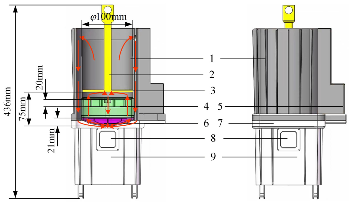
As shown in Figure 2, the 3D structural model of EHT is mainly composed of the upper shell, piston rod, piston, guide plate, impeller, lower shell, and drive motor. When the EHB releases the brake, the impeller of the EHT rotates at high speed, driven by the motor, driving the fluid at its bottom to rotate around the axial direction and diffuse along the radial direction at the same time; then, the fluid flows upward along the axial direction from the area between the blades of the guide plate to the piston bottom to provide the piston with an upward protruding hydraulic force; and finally, it flows downward along the axial direction along the central hole of the guide plate to the impeller top and enters the area between the vanes of the guide plate again to form an upward axial circulating vortex flow, which provides the piston with continuous hydraulic pressure, thus driving brake–release of the EHB.

In addition, since the fluid motion between the bottom of the piston and the top of the impeller of the EHT simultaneously includes rotational motion in the circumferential direction, and radial and axial rectilinear flow, local vortex structures inevitably emerge when the fluid flows in the area between the guide plate and the impeller and in the area between the guide plate blades, which will lead to loss of energy in the fluid of the EHT, thus weakening the output force of the EHT and degrading the braking performance of the EHB. Therefore, it is necessary to study the fluid flow characteristics and vortex characteristics of EHT.

3.2. Numerical Analysis of Flow Field of EHT

3.2.1. Governing Equations and Turbulence Models

In order to explore the fluid flow characteristics and vortex characteristics of the EHT, a simulation study was conducted using the Fluent software. The governing equations describing the fluid flow field distribution of the EHT include the continuity equation, the momentum conservation equation, the turbulent kinetic energy equation, and the turbulent dissipation rate equation.

The continuity equation and the momentum conservation equation are as follows:

$${\displaystyle \frac{\partial u}{\partial x}}+{\displaystyle \frac{\partial v}{\partial y}}+{\displaystyle \frac{\partial w}{\partial z}}=0$$

(1)

$$\left\{\begin{array}{c}{\displaystyle \frac{\partial u}{\partial t}}+u{\displaystyle \frac{\partial u}{\partial x}}+v{\displaystyle \frac{\partial u}{\partial y}}+w{\displaystyle \frac{\partial u}{\partial z}}=F_x+{\displaystyle \frac{\mu }{\rho }}\left({\displaystyle \frac{{\partial }^{2}u}{\partial x^2}}+{\displaystyle \frac{{\partial }^{2}u}{\partial y^2}}+{\displaystyle \frac{{\partial }^{2}u}{\partial z^2}}\right)\\ {\displaystyle \frac{\partial v}{\partial t}}+u{\displaystyle \frac{\partial v}{\partial x}}+v{\displaystyle \frac{\partial v}{\partial y}}+w{\displaystyle \frac{\partial v}{\partial z}}=F_y+{\displaystyle \frac{\mu }{\rho }}\left({\displaystyle \frac{{\partial }^{2}v}{\partial x^2}}+{\displaystyle \frac{{\partial }^{2}v}{\partial y^2}}+{\displaystyle \frac{{\partial }^{2}v}{\partial z^2}}\right)\\ {\displaystyle \frac{\partial w}{\partial t}}+u{\displaystyle \frac{\partial w}{\partial x}}+v{\displaystyle \frac{\partial w}{\partial y}}+w{\displaystyle \frac{\partial w}{\partial z}}=F_z+{\displaystyle \frac{\mu }{\rho }}\left({\displaystyle \frac{{\partial }^{2}w}{\partial x^2}}+{\displaystyle \frac{{\partial }^{2}w}{\partial y^2}}+{\displaystyle \frac{{\partial }^{2}w}{\partial z^2}}\right)\end{array}\right.$$

(2)

where x, y, and z are the coordinate components; t is the time (s); ρ is the density of the fluid (kg/m³); μ is the dynamic viscosity of the fluid (Pa·s); F_x, F_y, and F_z are the three volume force components in the rectangular coordinate system (N); and u, ν, and w are the three velocity components in the rectangular coordinate system (m/s).

The RNG k-ε model is adopted to describe the turbulent flow field of EHT. Although it shares a similar formulation with the standard k-ε model, the RNG version revises the turbulent viscosity formula and optimizes the dissipation rate transport equation and relevant model closure coefficients. These improvements enable it to handle complex rotational flow with large streamline curvature. Furthermore, this model shows prominent performance in simulating rotating flow, flow separation, and flow fields with high strain rates and can precisely capture vortex generation and evolution inside the rotating thruster. It is therefore well suited for the present flow simulation.

The turbulence kinetic energy k equation and the turbulence dissipation rate ε equation are as follows:

Turbulent kinetic energy k equation:

$${\rho }_1{\displaystyle \frac{\partial k}{\partial t}}+{\rho }_1{\displaystyle \frac{\partial }{\partial x_i}}\left(k{u}_i\right)={\displaystyle \frac{\partial }{\partial x_j}}\left({\alpha }_k\left({\mu }_1+{\mu }_t\right){\displaystyle \frac{\partial k}{\partial x_j}}\right)+G_k-{\rho }_1\epsilon$$

(3)

Turbulence dissipation rate ε equation:

$${\rho }_1{\displaystyle \frac{\partial \epsilon }{\partial t}}+{\rho }_1{\displaystyle \frac{\partial }{\partial x_i}}\left(\epsilon u_i\right)={\displaystyle \frac{\partial }{\partial x_j}}\left({\alpha }_{\epsilon }\left({\mu }_1+{\mu }_t\right){\displaystyle \frac{\partial \epsilon }{\partial x_j}}\right)+C_{1\epsilon }{\displaystyle \frac{\epsilon }{k}}{G}_k-C_{2\epsilon }{\rho }_1{\displaystyle \frac{{\epsilon }^2}{k}}$$

(4)

where u_i is the velocity component (m/s); x_i and x_j are the coordinate components (m); μ₁ is the hydrodynamic viscosity (Pa·s); μ_t is the turbulent viscosity coefficient (Pa·s); ρ₁ is the density of the fluid (kg/m³); C_1ε and C_2ε are empirical coefficients; G_k is the generation term of turbulence kinetic energy k caused by average velocity gradient; and α_k and α_ε are inverses of the turbulent Prandtl number related to the turbulent kinetic energy k and the dissipation rate ε, respectively.

Based on experience, the values of relevant parameters of the calculation model are as follows: C_1ε = 1.42 and C_2ε = 1.68.

3.2.2. Parameters of Numerical Analysis Model

Transient analysis is adopted for the numerical investigation of the fluid flow characteristics and vortex structures within the EHT. The density and viscosity of the fluid at different operating temperatures, which are used as boundary conditions in the simulation, are shown in

Table 1. The density and viscosity of the fluid at different operating temperatures.

Temperature	Density	Viscosity
0 °C	872 kg/m3	101.5 Pa·s
10 °C	866 kg/m3	76.5 Pa·s
20 °C	869 kg/m3	54.5 Pa·s

. All simulations are performed using ANSYS Fluent 2021 R1. Pressure-based implicit solver is employed, with the SIMPLE algorithm for pressure–velocity coupling. The convective terms of the turbulent kinetic energy and turbulent dissipation rate are discretized using the second-order upwind scheme, with a residual convergence criterion of 10⁻⁶. The density and dynamic viscosity of the fluid are set to 866 kg/m³ and 76.5 Pa·s, respectively. The impeller is defined as a rotating wall with a rotational speed of 300 rad/s about its axis, while all other fluid domain walls are treated as no-slip walls. To resolve the boundary layer accurately, the y+ value on all walls is controlled below 5, corresponding to a low-Reynolds-number near-wall treatment. The simulation adopts a time step of 1.0 × 10⁻³ s and a total simulation duration of 0.5 s. Within each time step, the solution is iterated until residuals meet the convergence criterion.

3.2.3. Mesh Independence Test

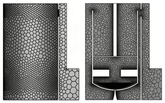
The fluid domain model of the EHT is divided using a polyhedral mesh approach, and key areas including the impeller, the bottom connection area of the impeller, and the blades of the guide plate are locally mesh-refined to ensure the calculation accuracy and reliability, as shown in Figure 3.

The quality of the mesh affects the accuracy of the numerical simulation results. Excessively dense meshes increase the computing time. In order to improve the efficiency of simulation calculation and effectively capture the flow details of fluid in the EHT, the geometric feature dimensions of mesh elements are set as 1.2 mm, 1.6 mm, and 2.0 mm, respectively. The mesh independence test results shown in

Table 2. Data of Mesh Independence Verification.

Serial Number	Element Number	Piston Bottom Pressure (MPa)	Simulation Error (%)
1	10,043,090	0.0962	0.31
2	6,212,859	0.0968	0.00
3	5,270,888	0.0965	0.21

are obtained by comparing the corresponding mesh element numbers as 10,043,090, 6,212,859, and 5,270,888, respectively. It can be seen from Table 2 that the overall influence of the number of mesh elements of the EHT fluid domain on the solution results is within 0.35% for a given number of mesh elements. On the premise of satisfying computational accuracy, in order to reduce the workload of simulation calculation, the mesh model of EHT with 5,270,888 mesh elements is selected to study the flow field characteristics.

3.2.4. Numerical Analysis Results and Analysis

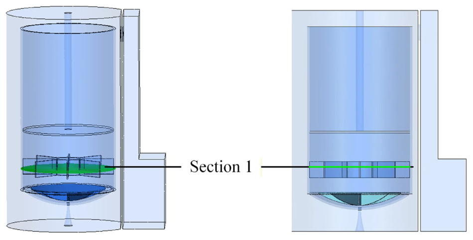
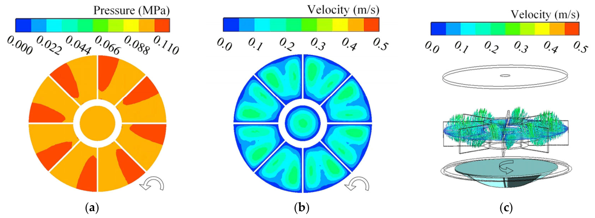
As the guide plate of the EHT is located between the impeller and the piston, local flow characteristics depend on the fluid flow state at the impeller and have a direct impact on the fluid flow state at the bottom of the piston. Thus, the radial Section 1 of the guide plate shown in Figure 4 is selected as the monitoring surface, and the fluid pressure contour, velocity contour, and velocity vector diagram at Section 1 are obtained through analysis, as shown in Figure 5, where the arrow direction indicates the rotation direction of the impeller.

Figure 5a shows that the fluid pressure between the two blades of the guide plate of the EHT increases gradually along the impeller rotation direction because the flow velocity of the fluid under the action of the impeller is the combined velocity of the radial velocity and the axial rotational velocity, and this combined velocity makes the fluid flow along the axial direction of the guide plate and deflect toward the impeller’s rotating direction when flowing into the guide plate. Figure 5b shows that the fluid flow velocity at the guide plate of the EHT changes regularly along the circumferential direction of the guide plate. The fluid flow velocity between two blades of the guide plate is higher along the circumferential direction on both sides and lower in the middle. Meanwhile, it can be seen that the fluid flow velocity at the central axis of the guide plate is higher. From Figure 5c, it can be seen that the fluid between the blades of the guide plate flows in the opposite direction along the circumferential direction at both ends, that is, fluid on one side flows axially upward and the fluid on the other side flows downward along the axial direction. The fluid at the center axis of the guide plate flows down along its axial direction.

From the above analysis, it can be seen that there is a strong vortex in the EHT that enters the piston bottom through the outer area of the guide plate and flows back to the impeller top from the central axis of the guide plate. This vortex can provide effective pressure and flow for the piston to stretch out. In addition, between the two blades of the guide plate, there is a weak vortex formed by a part of the fluid circulating back to the bottom of the guide plate and flowing upward together with the fluid discharged from the impeller. This vortex mainly occurs between the two blades of the guide plate; hence, it barely contributes to piston extension and induces extra hydraulic energy loss.

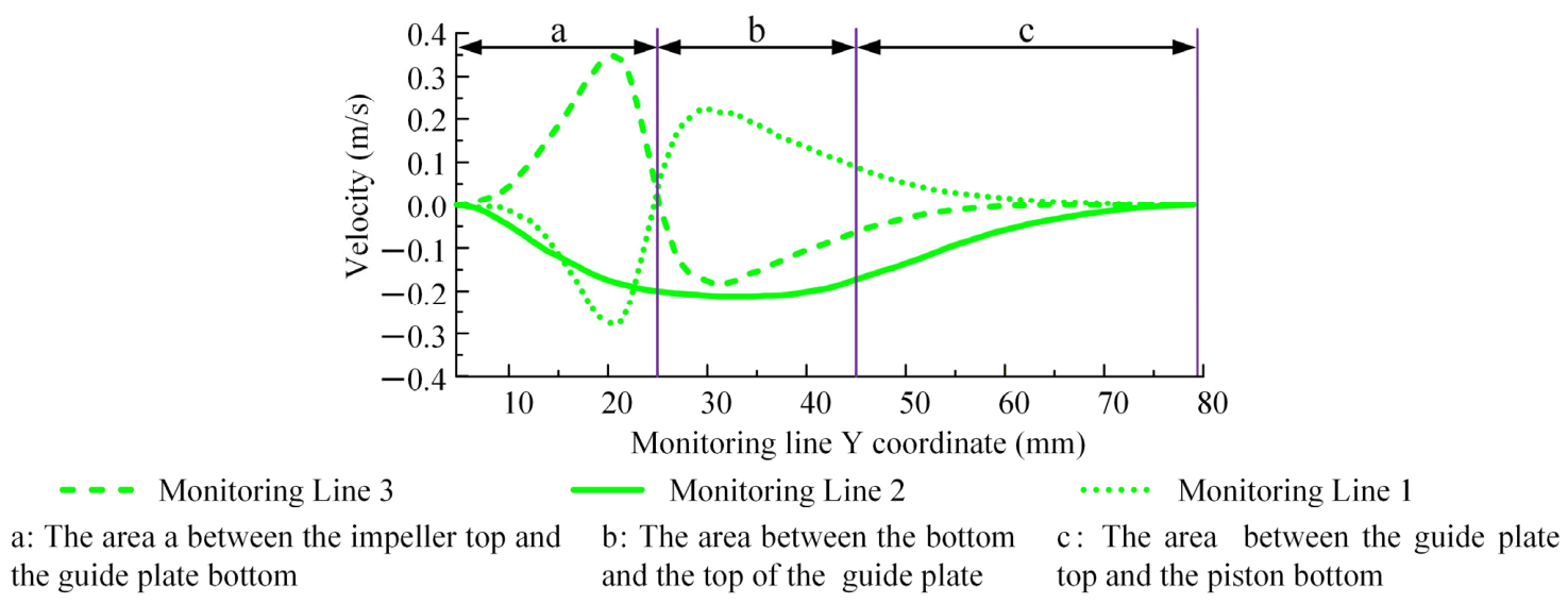
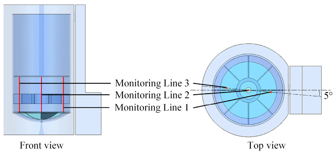
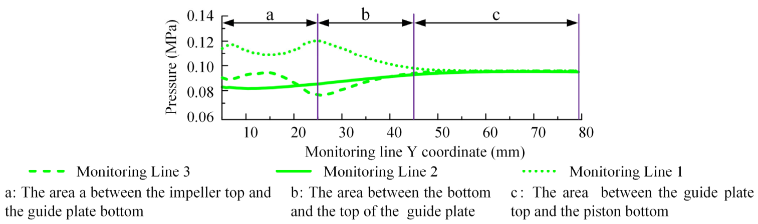
In order to quantitatively and continuously analyze the fluid pressure distribution characteristics of the three key axis directions in the EHT, three axial monitoring lines as shown in Figure 6 are established respectively and the fluid pressure distribution at each monitoring line is monitored. Monitoring line 1 is the axial line passing through the area with high fluid pressure between two blades of the guide plate shown in Figure 5a, monitoring line 2 is the central axis of the EHT, and monitoring line 3 is the axial line passing through the area with low fluid pressure between two blades of the guide plate shown in Figure 5a. The axial coordinate Y range of each monitoring line is 4~79 mm, where Y = 4~25 mm is area a between the impeller top and the guide plate bottom; Y = 25~45 mm is area b between the bottom and the top of the guide plate; and Y = 45~79 mm is area c between the guide plate top and the piston bottom. Owing to the blocking effect of guide plate blades in the horizontal direction of the top view of the EHT, when establishing the axial monitoring line, a point 5° offset from the horizontal radial line on the equal-diameter circle in Figure 6 is selected to avoid the guide plate blades.

The pressure distribution on monitoring line 1, monitoring line 2, and monitoring line 3 is obtained through analysis, as shown in Figure 7. It can be seen from the figure that in area a between the impeller top and the guide plate bottom, the fluid pressure along monitoring line 1 first increases, then decreases, and then increases, while the fluid pressure at monitoring line 3 shows a trend of decreasing first, then increasing, and then decreasing. The fluid pressure curves of monitoring line 3 and monitoring line 1 present a symmetrical distribution, and the fluid pressure at monitoring line 3 is obviously lower than that at monitoring line 1, which indicates that the fluid circulation flow from monitoring line 1 to monitoring line 3 exists at area a. In area b and area c between the bottom of the guide plate and the bottom of the piston, the fluid pressure curves at monitoring line 3 and monitoring line 1 also change symmetrically with each other, and the fluid pressure at monitoring line 3 is significantly lower than that at monitoring line 1, which indicates that there is fluid circulation flow from monitoring line 1 to monitoring line 3 in area b and area c. It can also be seen from Figure 7 that when the fluid flows to the bottom of the piston (Y = 79 mm), the pressure of the three monitoring lines is basically the same. At this time, the fluid pressure drives the piston to stretch out to realize the brake–release process. In addition, Figure 7 shows that the fluid pressure at monitoring line 1 of area a, area b, and area c is higher than the fluid pressure at monitoring line 2, which indicates that there is fluid circulation flow from monitoring line 1 to monitoring line 2 in area a, area b, and area c.

It can be seen from Bernoulli’s principle that the flow velocity of the three circulating flow patterns is directly related to the fluid pressure difference between the corresponding monitoring lines. The flow velocity distribution along the Y-axis of fluid in each area obtained through analysis is shown in Figure 8. The positive value represents the flow along the positive direction of the Y-axis, and the negative value represents the flow along the negative direction of the Y-axis.

Figure 8 shows that in area a between the impeller top and the guide plate bottom, with the increase in the Y-axis coordinate value, the fluid at monitoring line 1 flows along the negative direction of Y-axis and the velocity gradually increases from 0 m/s and subsequently decreases to 0 m/s, while the fluid at monitoring line 3 flows along the positive direction of Y-axis and the velocity gradually increases from 0 m/s and subsequently decreases to 0 m/s, indicating the presence of vortex α from monitoring line 3 to line 1. The vortex is formed because the fluid is driven by the impeller rotation, which is not conducive to the transmission of fluid to the piston bottom.

In area b and area c, the fluid at monitoring line 1 flows in the positive direction along the Y-axis and the velocity gradually increases from 0 m/s and subsequently decreases to 0 m/s, while the fluid at monitoring line 3 flows in the negative direction along the Y-axis and the velocity gradually increases from 0 m/s and subsequently decreases to 0 m/s, which indicates that there is a vortex flow β from monitoring line 1 to monitoring line 3 in this area. This vortex is formed due to the blocked fluid flow at the guide plate blades, which also forms an impediment to the fluid transmission to the piston bottom.

In addition, Figure 8 shows that when the fluid flows to the bottom of the piston (Y = 79 mm), the fluid velocity of the three monitoring lines is reduced to 0 m/s, and the fluid dynamic pressure is converted into static pressure to push the piston out. At the same time, Figure 8 shows that the fluid at monitoring line 2 at area a, area b, and area c flows in the negative direction along the Y-axis, and the velocity gradually increases from 0 m/s and subsequently decreases to 0 m/s, which indicates that there is a vortex flow γ from monitoring line 1 and monitoring line 3 to monitoring line 2 in this area. This vortex provides stable pressure for piston extension and is the core working flow field of the EHT.

It can be seen from the comprehensive analysis that among the above three types of vortices, vortex α and vortex β not only block the fluid delivery to the bottom of the piston but also consume extra energy, whereas vortex γ improves the operating performance of the EHT.

4. Analysis of Vortex Characteristics of EHT

From the above analysis, it can be seen that the three types of vortices have an important impact on the working performance of the EHT. However, different motor speeds have a direct impact on the fluid flow state inside the EHT. In addition, in cold regions of China, the working environment temperature difference of EHT is large, which directly affects the viscosity of fluid in the EHT, thus affecting the fluid flow state in the EHT. Therefore, it is necessary to conduct in-depth research and analysis on the three types of vortices characteristics at different motor speeds and fluid viscosities.

4.1. Influence of Fluid Viscosity on Vortex Characteristics of EHT

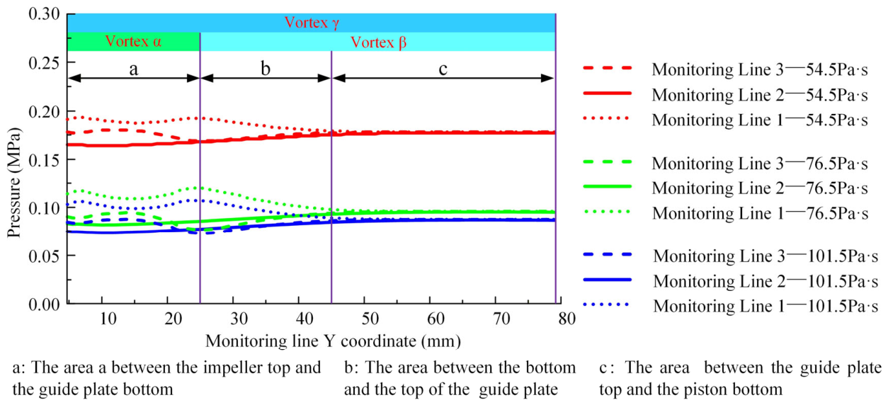
Due to the wide application areas of the EHB and the large range of temperature changes in its working environment, temperature variations directly affect the viscosity of the fluid inside the thruster, which in turn influences the internal vortex characteristics. This is critical for operational reliability and safety. The fluid pressure distribution of monitoring line 1, monitoring line 2, and monitoring line 3 at the viscosity of 54.5 Pa·s, 76.5 Pa·s, and 101.5 Pa·s is obtained through analysis, as shown in Figure 9. It can be seen from the figure that peak pressure at each monitoring line shows an inverse correlation to the fluid viscosity. As the fluid viscosity increases from 54.5 Pa·s to 101.5 Pa·s, the average pressure at the bottom of the piston decreases from 0.178 MPa to 0.096 MPa, deteriorating the overall EHT performance. Meanwhile, Figure 9 shows that the pressure fluctuation amplitude of all monitoring curves reduces synchronously with the increase in fluid viscosity, which indicates that the increase in fluid viscosity will weaken the pressure gradient of the fluid in the EHT, thus restricting fluid dynamic performance.

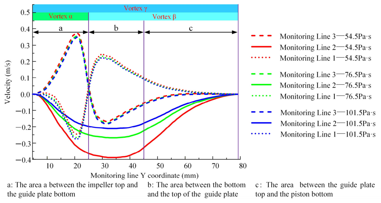
The fluid velocities at monitoring line 1, monitoring line 2, and monitoring line 3 at the viscosities of 54.5 Pa·s, 76.5 Pa·s, and 101.5 Pa·s are obtained through analysis, as shown in Figure 10. It can be seen from the figure that with the increase in viscosity, the peak velocities of vortex α, vortex β, and vortex γ all show decreasing trends. This is because the increase in fluid viscosity will lead to an increase in the flow resistance of the fluid inside the EHT.

By conducting quantitative analysis on the velocity distribution curves of monitoring line 1, monitoring line 2, and monitoring line 3 under different viscosities, as shown in Figure 10, the peak values and variations in the velocities of vortex α, vortex β, and vortex γ at viscosities of 54.5 Pa·s and 101.5 Pa·s are presented in

Table 3. Peak velocities of vortex α, vortex β, and vortex γ under different fluid viscosities.

	Vortex	α	β	γ	α/γ	β/γ
Viscosity
54.5 Pa·s		0.37 m/s	0.25 m/s	0.39 m/s	94.9%	64.1%
101.5 Pa·s		0.35 m/s	0.22 m/s	0.21 m/s	166.7%	104.8%
Decrease rate		5.4%	12.0%	46.2%

. It can be seen from the table that when the fluid viscosity is 54.5 Pa·s, the proportion of the peak velocity of vortex α to that of vortex γ is 94.9%, and the proportion of the peak velocity of vortex β to that of vortex γ is 64.1%. However, when the fluid viscosity rises to 101.5 Pa·s, the proportion of the peak velocity of vortex α to that of vortex γ sharply increases to 166.7%, and the proportion of the peak velocity of vortex β to that of vortex γ rapidly increases to 104.8%.

By analyzing the peak values of the above-mentioned vortex velocities, it can be seen that as the viscosity of the fluid increases from 54.5 Pa·s to 101.5 Pa·s, the peak velocity of vortex γ decreases by 46.2%, which is much greater than the decrease in the peak velocities of vortex α (5.4%) and vortex β (12.0%). This indicates that in the tested viscosity scope, although an increase in fluid viscosity weakens the intensity of harmful vortex α and vortex β, its effect on weakening vortex γ is more significant, further reducing the working performance of the EHT.

From the above analysis, it can be concluded that the fluid viscosity regulates the pressure gradient and velocity distribution of the internal flow field by changing the viscous resistance of the fluid, thereby influencing the intensities of the three types of vortices. Among them, the intensities of vortex α, vortex β, and vortex γ decrease overall as the viscosity increases, but the weakening trend of vortex γ is more pronounced. This law provides theoretical support to adjust fluid viscosity parameters under different temperature conditions. That is, while weakening the harmful vortices, the beneficial vortex can be ensured to support the improvement in thruster performance by adjusting the fluid viscosity.

4.2. Influence of Motor Speed on Vortex Characteristics of EHT

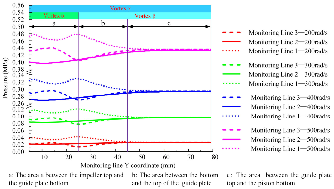
The motor speed, as the core parameter for driving the rotor to rotate, directly determines fluid kinetic energy and affects the formation and development of vortices. The conventional operating speed of the EHT motor is 300 rad/s, and the speed range under different working conditions is 200–500 rad/s, which covers regular and extreme working rotational speeds of the EHT. Through analysis, the fluid pressures at monitoring lines 1, monitoring lines 2, and monitoring lines 3 when the motor speed is 200 rad/s, 300 rad/s, 400 rad/s, and 500 rad/s are shown in Figure 11. As can be seen from the figure, as the motor speed increases from 200 rad/s to 500 rad/s, the average pressure at the bottom of the piston increases from 0.0263 MPa to 0.435 MPa, which is conducive to improving the working characteristics of the EHT. At the same time, as the motor speed increases, the pressure peaks at the three monitoring lines all show an upward trend, and the pressure difference between the monitoring lines (the difference between the maximum and minimum pressures) gradually increases with increasing rotational speed, indicating that the increase in motor speed significantly enhances radial pressure gradient of the fluid, thereby increasing the intensity of each vortex.

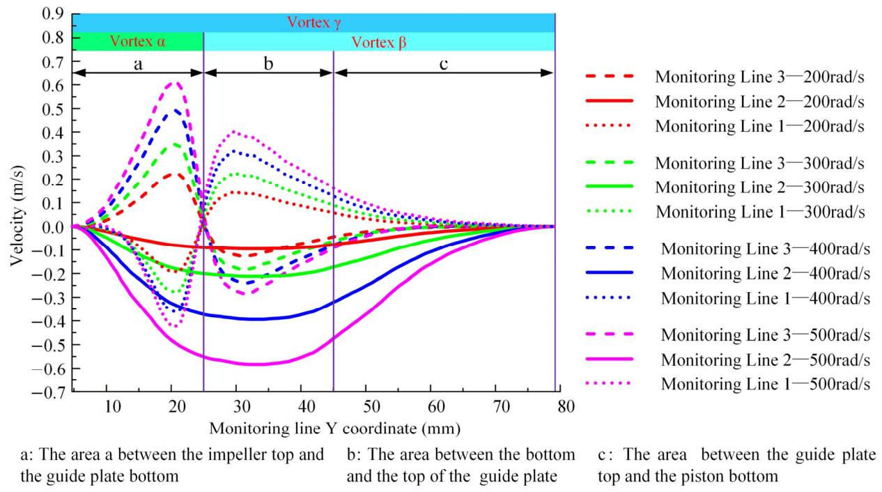
The fluid velocities at monitoring lines 1, monitoring lines 2, and monitoring lines 3 under motor speeds of 200 rad/s, 300 rad/s, 400 rad/s, and 500 rad/s are shown in Figure 12. From the figure, it can be seen that as the motor speed increases, the peak values of the velocities of the vortex α, vortex β, and vortex γ all show an increasing trend. This is because the increase in motor speed simultaneously enhances the kinetic energy of fluid flow in each area. At the same time, Figure 12 shows that the difference in peak velocities between vortex α and vortex β (the difference in peak velocities between monitoring lines 1 and monitoring lines 3) approximately increases linearly with increasing rotating speed. The axial velocity component difference of vortex γ increases slowly in the medium and low motor speed range and increases more rapidly in the high motor speed range. This indicates that the increase in motor speed has a more significant enhancing effect on the vortex γ.

Through quantitative analysis of the velocity distribution curves of monitoring line 1, monitoring line 2, and monitoring line 3 under different motor speeds, as shown in Figure 12, the peak values and variations in the velocities of vortex α, vortex β, and vortex γ at motor speeds of 200 rad/s and 500 rad/s are shown in

Table 4. Peak velocities of vortex α, vortex β, and vortex γ under different motor speeds.

	Vortex	α	β	γ	α/γ	β/γ
Motor Speed
200 rad/s		0.23 m/s	0.15 m/s	0.09 m/s	255.6%	166.7%
500 rad/s		0.62 m/s	0.41 m/s	0.58 m/s	106.9%	70.7%
Increase rate		169.6%	173.3%	544.4%

. It can be seen from the table that when the motor speed is 200 rad/s, the proportion of the peak velocity of vortex α to that of vortex γ is 255.6%, and the proportion of the peak velocity of vortex β to that of vortex γ is 166.7%. However, when the motor speed rises to 500 rad/s, the proportion of the peak velocity of vortex α to that of vortex γ rapidly decreases to 106.9%, and the proportion of the peak velocity of vortex β to that of vortex γ sharply decreases to 70.7%. By analyzing the peak values of the above-mentioned vortex velocities, it can be seen that as the motor speed increases from 200 rad/s to 500 rad/s, the peak velocity of vortex γ increases by 544.4%, which is much greater than the increase in the peak velocity of vortex α (169.6%) and vortex β (173.3%). This indicates that within the selected motor speed range, although increasing the motor speed does intensify the harmful vortex α and vortex β, its effect on enhancing the intensity of vortex γ is more significant, thereby further improving the performance of the EHT.

Furthermore, considering the characteristic that vortex α and vortex β directly cause energy loss in the fluid and are not conducive to improving the braking performance of the EHT, it can be concluded that although increasing the motor speed is more beneficial for enhancing the intensity of the beneficial vortex γ and improving the propulsion efficiency, it will also exacerbate the energy loss of the harmful vortex α and vortex β. Therefore, in practical applications, it is necessary to balance the dual effects of motor speed on the characteristics of vortices and determine the optimal motor speed range that can both ensure the release of braking torque and minimize energy loss, and avoid blindly adopting excessively high rotational speeds that reduce energy efficiency.

5. Discussion

5.1. Formation Mechanism of Vortex and Research Significance

The three vortex structures identified in this study originate from combined effects of fluid rotation, flow blockage, and pressure gradient within the EHT flow field. Vortex α occurs in the outer recirculation zone due to the shear between radial and axial flows driven by the impeller, which blocks upward flow and increases local dissipation. Vortex β appears near the guide vanes as a result of flow separation and local blockage, consistent with common energy dissipation mechanisms in rotating hydraulic machinery. Vortex γ forms a stable circulating flow between the impeller, vanes, and piston bottom, providing effective driving support for piston extension.

These vortices collectively determine the efficiency and stability of the brake–release process. Under low-temperature conditions, elevated fluid viscosity weakens the driving capacity of beneficial vortex γ while failing to suppress harmful vortices α and β, leading to insufficient piston power and delayed brake–release. Most previous studies have focused on braking performance rather than the internal flow mechanism during brake–release. The present work fills this research gap by revealing vortex-dominated flow physics, providing a mechanical basis for improving low-temperature performance.

5.2. Regulation Mechanism and Balancing Strategy of Key Parameters

5.2.1. Regulation Effect of Fluid Viscosity

Fluid viscosity influences vortex behavior mainly by modifying flow resistance and momentum diffusion. Higher viscosity increases internal friction, reduces flow uniformity, and suppresses all vortices. Notably, the beneficial vortex γ is more sensitive to viscosity changes, implying excessive viscosity directly damages the main driving flow. This trend highlights the importance of fluid selection at low temperatures: viscosity should be limited to a reasonable range to suppress harmful vortices while preserving the dominance of vortex γ.

5.2.2. Dual Effects of Motor Speed

Motor speed governs total energy input and internal pressure distribution of the entire system. Increasing speed strengthens all vortices, but the growth rate of vortex γ is more significant, which helps maintain its dominant role. However, higher speed also intensifies shear loss and recirculation intensity in vortices α and β, reducing overall hydraulic efficiency. Thus, simply boosting rotating speed is not an optimal design choice. In engineering practice, speed should be matched to temperature, load, and response time to strike a reasonable balance between driving force and energy loss.

5.3. Limitations of This Study

This study has several inherent limitations that should be objectively stated to guarantee the rationality and applicability of the conclusions. Notably, this work lacks experimental validation or comparison with published experimental data, and no turbulence model sensitivity analysis is performed. First, all results are obtained from transient CFD numerical simulations, and experimental tests and field measurements are not available in the current stage. Although grid independence verification has been conducted, the mesh resolution near the wall and vortex core regions is still limited by computational resources. The y+ value and near-wall treatment may also affect the prediction of wall shear stress and boundary layer development. Second, the simulation is carried out on a fixed EHT geometric model without considering the machining errors, assembly clearances, and component wear in practical engineering. Third, the parametric analysis only selects three typical low-temperature viscosity values and a limited speed range, which cannot fully cover all operating conditions of the equipment. In addition, some secondary factors such as cavitation effect, internal fluid temperature gradient, and unsteady boundary disturbance are not considered in this study. Future research will carry out prototype experiments and multi-turbulence model comparative analyses, adaptive mesh refinement, and wider parameter range analyses to further improve the reliability and engineering practicability of the conclusions.

6. Conclusions

During the process of releasing the brake of the investigated EHT structure, three typical vortex configurations are observed: vortex α between the impeller top and the guide plate bottom, vortex β between the guide plate bottom and the piston bottom, and vortex γ between the impeller top and the piston bottom. Under the simulated flow conditions, vortex α and vortex β cause energy loss of the fluid and weaken the overall EHB braking performance, while vortex γ provides a stable liquid pressure for the piston to extend and is the core flow field that ensures the performance of releasing the brake. The main conclusions are summarized as follows:

(1) Within the investigated viscosity range, fluid viscosity has a significant regulatory effect on vortex characteristics: as the viscosity increases from 54.5 Pa·s to 101.5 Pa·s, the intensities of all three types of vortices weaken, and the weakening effect on vortex γ is more pronounced. The average pressure at the bottom of the piston decreases from 0.178 MPa to 0.096 MPa. Therefore, in low-temperature conditions, it is necessary to select an appropriate viscosity of the fluid medium within the investigated numerical range to balance the requirements for inhibiting harmful vortices and retaining beneficial vortices.

(2) The motor speed is the core dynamic parameter that affects the characteristics of vortices within the investigated speed range. As the speed increases, the intensities of all three vortices increase, and the growth of vortex γ is more significant. The average pressure at the bottom of the piston increases from 0.0263 MPa to 0.435 MPa. Therefore, it is necessary to determine the optimal motor speed range for the studied EHT configuration to avoid the decline in energy efficiency caused by simply pursuing a high speed.

(3) Within the limitations of the present numerical study and the investigated geometric structure, this study reveals the vortex formation mechanism and key parameter regulation laws of the EHT during brake–release. The conclusions can support fluid selection and speed matching for similar EHT structures under comparable working conditions. By suppressing harmful vortices while maintaining the intensity of the beneficial vortex, the brake–release performance and energy efficiency of the EHB can be effectively improved.

References

1. Jiang, C.J.; Tian, S.T.; Kong, X.H. Simulation of Electro-hydraulic Disc Brake Based on ADAMS. Mech. Eng. Autom. 2015, 12, 80–81. [Google Scholar]
2. Fan, H.C. The application of electric hydraulic normally closed brake in crane slewing mechanism. China Sci. Technol. Inf. 2018, 1, 48–49. [Google Scholar] [CrossRef]
3. Yang, J.; Gong, Z.; Xia, S.; Luo, K.; Li, H. Numerical analysis on influence of guide vanes on performance of centrifugal pump acting as hydraulic turbine. J. Drain. Irrig. Mach. Eng. 2014, 32, 113–118. [Google Scholar] [CrossRef]
4. Jiang, X.; Gao, M.; Song, J.J. Research on brake torque regulation of electro-hydraulic brake. Coal Eng. 2017, 49, 122–124. [Google Scholar] [CrossRef]
5. Zhao, B. Integration Method of Thermal Convection Characteristics Prediction for Unsteady Laminar Flows during Initial Braking Stage of Wet Brakes. J. Mech. Eng. 2020, 56, 198–207. [Google Scholar] [CrossRef] [Scilit]
6. Han, W.; Xiong, L.; Yu, Z.P. Braking pressure control in electro-hydraulic brake system based on pressure estimation with nonlinearities and uncertainties. Mech. Syst. Signal Process. 2019, 131, 703–727. [Google Scholar] [CrossRef] [Scilit]
7. Han, W.; Xiong, L.; Yu, Z.; Zhuo, G.; Leng, B.; Xu, S. Integrated Pressure Estimation and Control for Electro-hydraulic Brake Systems of Electric Vehicles Considering Actuator Characteristics and Vehicle Longitudinal Dynamics. IEEE/ASME Trans. Mechatron. 2023, 28, 197–209. [Google Scholar] [CrossRef] [Scilit]
8. Han, W.; Xiong, L.; Yu, Z.P. Analysis and optimization of minimum hydraulic brake-by-wire system for wheeled vehicles based on queueing theory. IEEE Trans. Veh. Technol. 2021, 70, 12491–12505. [Google Scholar] [CrossRef] [Scilit]
9. Lignon, S.; Sinou, J.; Jezequel, L. Stability analysis and μ-synthesis control of brake systems. J. Sound Vib. 2006, 298, 1073–1087. [Google Scholar] [CrossRef] [Scilit]
10. Garcia-Leon, R. Thermal study in three vented brake discs, using the finite element analysis. Dyna 2017, 84, 19–27. [Google Scholar] [CrossRef] [Scilit]
11. Bai, Z.C.; Lv, X.L. Structure and performance of disc-type magnetorheological fluid brake based on CFD. J. Nanjing Univ. Sci. Technol. 2018, 42, 474–483. [Google Scholar] [CrossRef]
12. Liu, C.Y.; Jiang, K.J.; Yi, F.Y. Numerical Analysis of Inner Flow Field for Cylindrical Magnetorheological Brake. J. Syst. Simul. 2011, 23, 628–631. [Google Scholar] [CrossRef] [Scilit]
13. Gu, X.B.; Su, W.S.; Bai, J.Y. Dynamic braking moment test for hoisting machinery based on speed-reduction method. Hoisting Conveying Mach. 2014, 6, 84–87. [Google Scholar]
14. Cai, L.N.; Sun, M.X.; Bao, D.H. Normally closed electric hydraulic caliper disc brake torque static test research. Constr. Mech. 2014, 35, 58–59. [Google Scholar]
15. Shen, W. Research on Intelligent Brake Control System Based on Electric Hydraulic Push Rod Brake. Master’s Thesis, Beijing Technology and Business University, Beijing, China, 2005. [Google Scholar]
16. Wang, S.L.; Wang, X.R.; Yuan, K.J. Energy analysis and energy efficiency improvement of electro-hydraulic drum brake. Anal. Res. 2018, 2, 135–138. [Google Scholar]
17. Junior, M.; Gerges, S.; Jordan, R. Analysis of brake squeal noise using the finite element method: A parametric study. Appl. Acoust. 2008, 69, 147–162. [Google Scholar] [CrossRef] [Scilit]
18. Rafiee, S.E.; Sadeghiazad, M.M. Three-Dimensional CFD Simulation of Fluid Flow inside a Vortex Tube on Basis of an Experimental Model- The Optimization of Vortex Chamber Radius. Int. J. Heat Technol. 2016, 34, 236–244. [Google Scholar] [CrossRef] [Scilit]
19. Rafiee, S.E. Experimental and thermo-dynamical analysis of fully turbulent gas flows in vortex tube- fluid, temperature and power separations, isentropic efficiency, coefficient of performance (COP). Int. Commun. Heat Mass Transf. 2022, 138, 106296. [Google Scholar] [CrossRef] [Scilit]
20. Rafiee, S.E.; Sadeghiazad, M.M. Experimental and 3D CFD analysis on optimization of geometrical parameters of parallel vortex tube cyclone separator. Aerosp. Sci. Technol. 2016, 63, 110–122. [Google Scholar] [CrossRef] [Scilit]
21. Cherepanov, V.; Liu, J.; Qian, Z. On the dynamics of the boundary vorticity for incompressible viscous flows. J. Sci. Comput. 2024, 99, 42. [Google Scholar] [CrossRef] [Scilit]
22. Pu, J.J.; Xiong, Y. Numerical study of hydrofoil tip vortex fluid field. Chin. J. Ship Res. 2017, 12, 8–13+26. [Google Scholar] [CrossRef]
23. Pu, J.J.; Xiong, Y.; Wang, R. Scaling Effects of Hydrofoil Tip Vortex Cavitation Inception. J. Shanghai Jiao Tong Univ. 2017, 51, 374–378. [Google Scholar] [CrossRef]
24. Berestova, S.A.; Prosviryakov, E.Y. An Inhomogeneous Steady-State Convection of a Vertical Vortex Fluid. Russ. J. Nonlinear Dyn. 2023, 19, 167–186. [Google Scholar] [CrossRef] [Scilit]
25. Cao, L.; Takamure, K.; Uchiyama, T. Numerical analysis of effect of Reynolds number on interaction of density-stratified fluid with a vortex ring. Phys. Fluids 2022, 34, 053314. [Google Scholar] [CrossRef] [Scilit]
26. Degawa, T.; Uchiyama, T. Numerical Simulation of Mixing by Interaction of a Vortex Ring with a Density Interface. J. Energy Power Eng. 2018, 12, 565–577. [Google Scholar] [CrossRef] [Scilit]
27. Koralewski, J. Influence of hydraulic oil viscosity on the volumetric losses in a variable capacity piston pump. Pol. Marit. Res. 2011, 18, 55–65. [Google Scholar] [CrossRef] [Scilit]
28. Gao, Y.; Gu, L.; Jiao, L. Effects of Oil Properties on Flow Pulsation of Axial Piston Pumps by Simulation Analysis. China Mech. Eng. 2017, 11, 1333–1338. [Google Scholar] [CrossRef]
29. Liu, J.; Zhao, B.; Gao, G.-J. Consider the Influence of Viscosity-temperature Characteristics on the Cavitation Jet of Axial Piston Pump. Chin. Hydraul. Pneum. 2021, 45, 35–42. [Google Scholar] [CrossRef]
Figure 1. EHB two-dimensional model. 1—Right side base. 2—Spring assembly. 3—Transmission shaft. 4—Left side base. 5—Support bolt. 6—Brake drum. 7—Left brake arm. 8—Retractable threaded rod. 9—Right brake arm. 10—Transmission plate. 11—EHT.
Machines 14 00669 g001
Figure 2. EHT three-dimensional model. 1—Upper shell. 2—Piston rod. 3—Piston. 4—Guide plate. 5—Oil storage box. 6—Impeller. 7—Lower shell. 8—Junction box. 9—Motor.
Machines 14 00669 g002
Figure 3. Fluid domain mesh model of the EHT.
Machines 14 00669 g003
Figure 4. Radial Section 1 schematic diagram.
Machines 14 00669 g004
Figure 5. The fluid pressure contour, velocity contour, and velocity vector diagram of Section 1. (a) Contour of fluid pressure. (b) Contour of fluid velocity. (c) Contour of fluid velocity.
Machines 14 00669 g005
Figure 6. Axial monitoring line 3, monitoring line 2, and monitoring line 1 schematic diagram.
Machines 14 00669 g006
Figure 7. Pressure distribution curves of monitoring line 1, monitoring line 2, and monitoring line 3.
Machines 14 00669 g007
Figure 8. Velocity distribution curves of monitoring line 1, monitoring line 2, and monitoring line 3.
Machines 14 00669 g008
Figure 9. Pressure distribution curves of monitoring line 1, monitoring line 2, and monitoring line 3 under different fluid viscosities.
Machines 14 00669 g009
Figure 10. Velocity distribution curves of monitoring line 1, monitoring line 2, and monitoring line 3 under different fluid viscosities.
Machines 14 00669 g010
Figure 11. Pressure distribution curves of monitoring line 1, monitoring line 2, and monitoring line 3 under different motor speeds.
Machines 14 00669 g011
Figure 12. Velocity distribution curves of monitoring line 1, monitoring line 2, and monitoring line 3 under different motor speeds.
Machines 14 00669 g012