Towards Safer and More Efficient Cooperative Vehicle Platooning: Map-Based Calibration of Centralised LQR Control

Abstract

This paper proposes a calibration-oriented framework for cooperative adaptive cruise control based on a linear quadratic regulator formulation. A simulation-based architecture is developed by integrating the controller with a nonlinear longitudinal platoon model that explicitly accounts for actuator saturation and tyre–road friction limits, enabling the analysis of platoon behaviour under realistic operating conditions. A systematic offline calibration methodology is introduced based on multidimensional performance maps, relating key performance indicators associated with collision avoidance, comfort, and energy efficiency to controller and spacing-policy tuning parameters. The map-based approach enables a structured exploration of competing objectives and provides a quantitative assessment of controller sensitivity. The results show that the proposed framework can identify calibration regions that preserve collision-free operation in safety-critical manoeuvres while maintaining satisfactory tracking and comfort-related performance. In addition, the off-nominal model parameters analysis confirms that the proposed calibration approach remains effective under heterogeneous operating conditions, including vehicle parametric variation of mass, rolling resistance coefficient and drag. Overall, the results support the use of the proposed methodology as a practical tool for robust and performance-oriented controller calibration.

1. Introduction

Advanced Driver Assistance Systems (ADASs) and automated driving technologies are increasingly recognised as key enablers for improving road safety and transport sustainability [1,2]. In parallel, the rapid development of connected and automated vehicles is promoting cooperative control strategies for mixed-traffic coordination, in which vehicle-level automation is supported by shared information and infrastructure-level coordination [3,4]. Within this context, vehicle platooning has emerged as one of the most promising cooperative driving applications, especially for freight transport, where multiple vehicles travel in a coordinated manner while maintaining short inter-vehicle distances through automation and vehicle-to-vehicle communication [5,6]. The interest in platooning is motivated by its potential to reduce fuel consumption and emissions through aerodynamic drag reduction, improve traffic flow, and mitigate driver workload during long operations [7,8,9,10,11]. These expected benefits have stimulated extensive international research activity, from the early pioneering projects such as ARAMIS and PROMETHEUS to later initiatives such as CHAUFFEUR, PATH, KONVOI, Energy-ITS, SARTRE, CONCORDA, Sweden4Platooning, and ENSEMBLE, which progressively moved the field from conceptual feasibility towards real-world deployment and interoperability [12,13,14,15,16,17,18].

A substantial part of the literature has focused on quantifying the energy-saving potential of platooning, particularly for heavy-duty vehicles. Experimental campaigns and Computational Fluid Dynamics (CFD) studies have consistently shown that close-spacing operation can significantly reduce aerodynamic drag, with measurable benefits for both following and leading vehicles [7,15,19,20,21,22]. However, the achievable fuel benefit is not only determined by drag reduction; the adopted control strategy allows a smoother regulation of vehicle speed and inter-vehicle distance thus reducing unnecessary acceleration and deceleration events, thereby improving overall energy efficiency. From the control viewpoint, platooning systems are typically implemented through Adaptive Cruise Control (ACC) or Cooperative Adaptive Cruise Control (CACC) architectures [23,24]. In ACC, each vehicle reacts mainly to its predecessor using local sensing, whereas in CACC the control action also exploits exchanged information from other vehicles in the platoon using V2X technologies, allowing faster and more coordinated responses [25,26,27,28,29,30]. Many authors focus on another fundamental requirement in this context which is string stability, namely the ability of the platoon to attenuate disturbances as they propagate from the first to the last vehicle in the platoon [31,32]. This property is essential to prevent amplification of spacing or velocity errors along the vehicle string and is therefore closely related to both safety and traffic-flow quality. Previous studies have shown that conventional ACC does not generally guarantee string stability, whereas CACC can achieve significantly better disturbance attenuation thanks to the cooperative use of shared information [33,34].

Another key design choice concerns the spacing policy used to define the desired steady-state distance between consecutive vehicles [35]. Constant-spacing and constant-time-headway policies remain the most common formulations, although several variants have also been proposed, including delayed spacing, adaptive spacing, and traffic-oriented or human-inspired ones [32,36,37,38,39,40]. The spacing policy directly affects the balance among safety, comfort, road capacity, and energy efficiency. In parallel, a wide range of control techniques have been proposed for platooning, including classical PID-based approaches, robust $H_{\infty }$ formulations, Linear Quadratic Regulators (LQRs), Model-Predictive Control (MPC), and more recent machine-learning-based strategies [5,27,33,41,42,43,44,45,46]. Among these, LQR-based approaches are particularly attractive due to their compact formulation and their ability to balance tracking performance and control effort through the selection of weighting matrices [47]. Recent studies have addressed increasingly realistic platooning problems, including hierarchical cooperation architectures, safety-aware control formulations, and robustness to parametric uncertainty and model mismatch [48,49,50]. However, these advances have only rarely been translated into calibration-oriented design tools capable of explicitly identifying feasible and non-feasible parameter regions for low-complexity controllers intended for practical implementation.

Although the platooning literature has extensively addressed spacing policies, string stability, collision avoidance, and energy-efficient coordination, these topics have largely been investigated from the viewpoint of controller design or optimal planning rather than from that of controller calibration. In particular, low-complexity CACC architectures suitable for real-time implementation are still often tuned heuristically or assessed only under limited nominal conditions, while the combined effect of controller weights and spacing-policy parameters on collision avoidance, ride comfort, and energy-related performance remains insufficiently quantified when physical vehicle limits and off-nominal operating conditions are taken into account. This limitation is particularly relevant from a vehicle dynamics perspective, as actuator saturation, tyre–road friction variability, and vehicle parametric uncertainties (e.g., mass, rolling resistance, and aerodynamic drag) can significantly restrict the set of admissible calibrations.

In this context, the present work does not propose a new platooning controller, but rather a calibration-oriented framework for a centralised LQR-based CACC architecture.

Differently from standard LQR tuning or stability-region analysis, the proposed methodology combines closed-loop damping information with nonlinear time-domain simulations including actuator saturation, tyre–road friction limits, and performance indicators related to collision avoidance, comfort, and energy efficiency. In this sense, the maps are not intended as stability maps only, but as calibration maps supporting the selection of feasible controller settings under realistic vehicle operating constraints.

The main contributions of this work can be summarised as follows:

• A calibration-oriented methodology is proposed to reduce the LQR tuning problem to a limited set of physically interpretable parameters, namely $Q_0$, $R_0$, and $t_h$.
• Multidimensional performance maps are constructed to identify feasible and non-feasible tuning regions by combining collision-avoidance constraints with comfort, energy-efficiency, and tracking-performance indicators.
• The calibration procedure is evaluated on a nonlinear longitudinal platoon model including actuator saturation and tyre–road friction limits, so that the resulting controller configurations can be assessed beyond nominal linear-design conditions.
• The resulting calibration regions are further evaluated under representative off-nominal conditions, including vehicle-mass variability, rolling, and drag coefficient.
• A practical implementation is described, where the maps are used as an offline calibration database for fixed, conservative, or risk-dependent tuning selection.

The proposed framework is therefore intended as a practical design and calibration tool for a known centralised LQR/CACC architecture. It is not presented as a new control law, nor as a replacement for formal string-stability or general safety analyses, but as a structured methodology for identifying feasible and non-feasible calibration regions in a multi-objective and vehicle-dynamics-informed setting. The present study is intentionally developed and validated within a simulation-based framework, which enables a systematic and repeatable exploration of the controller calibration space under heterogeneous operating conditions. Experimental or hardware-in-the-loop validation is regarded as a natural extension of this work and is left for future research.

The paper is organised as follows. Section 2 introduces the platooning model and the adopted centralised LQR-based CACC strategy. Section 3 describes the key performance indicators used to construct the calibration maps. Section 4 presents the map-based calibration framework in terms of controller parameters and time headway. Section 5 discusses the calibration results under nominal and off-nominal vehicle conditions and introduces the practical implementation of the proposed map-based tuning approach. Finally, conclusions are drawn in Section 6.

2. CACC-Based Platooning Control Design

This section first describes the dynamic model of the vehicles forming the platoon and then introduces the platooning control strategy. The equations of motion governing the longitudinal dynamics of the vehicles are linearised and expressed in state-space form in order to simplify the subsequent closed-loop control design. More specifically, a Linear Quadratic Regulator (LQR) is adopted for the feedback control of the platoon. Before presenting the detailed mathematical formulation, the main assumptions and limitations underlying the proposed approach are reported below.

• The lead vehicle of the platoon is treated as an exogenous agent. It is not involved in the CACC control strategy and is therefore considered a source of disturbance to the controlled system. In this work, the lead vehicle is assumed to be driven either by a torque profile in open-loop or by Cruise-Control (CC) system designed to track a predefined speed reference.
• The string of follower vehicles is managed by an Electronic Centralised Control Unit (ECCU), which collects sensor measurements such as vehicle speed and inter-vehicle distance, required for full-state feedback control.
• The ECCU computes the reference speed and inter-vehicle distance to be maintained during driving and assigns these references to each follower vehicle in the platoon.
• The ECCU provides each follower vehicle with the torque command required to track the reference speed and maintain the desired inter-vehicle distance.
• Data exchange among vehicles and the ECCU is assumed to be instantaneous and free of communication delays or disturbances.
• The control law is formulated as a full-state feedback controller based on the LQR approach.

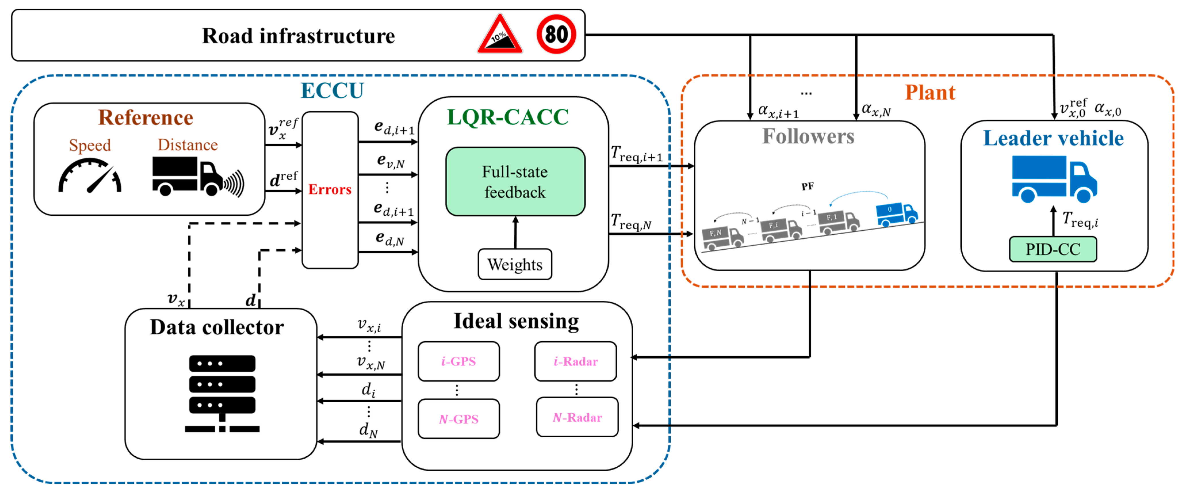
Figure 1 illustrates the high-level control architecture adopted for the cooperative driving simulations. The ECCU provides information on the reference speed, inter-vehicle distance setpoint, and road slope and collects measurements of vehicle speed and inter-vehicle distance from onboard sensors. Based on these measurements, the ECCU computes the inter-vehicle distance error and the speed error for each follower vehicle and forwards them to the CACC controller. The resulting feedback control actions are then applied to the platoon plant in the form of torque demands at the powertrain level for all the platoon vehicles. The mathematical description of the CACC algorithm is presented in the next section.

2.1. Vehicle Model

2.1.1. Nonlinear Longitudinal Dynamics

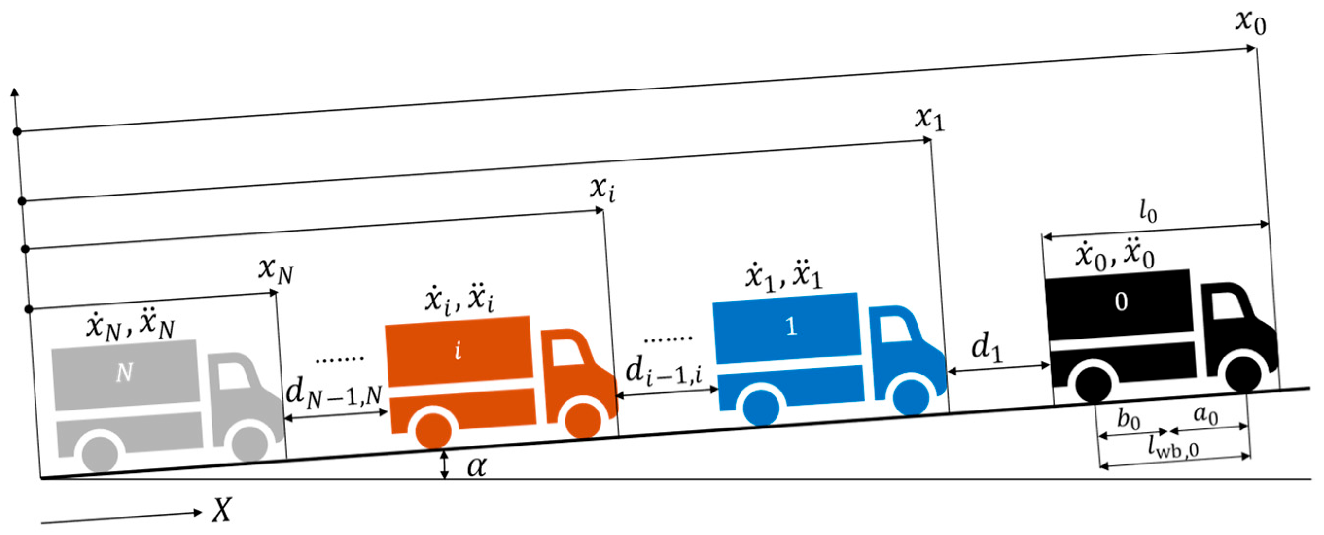
Let us consider a number of N Medium Duty Vehicles (MDVs), indexed by $i = 0, \dots , N$, represented by the mechanical scheme of Figure 2. The vehicle platoon is composed of a lead vehicle ($i=0$), while all the remaining vehicles are referred to as followers ($i=1$), where the subscript _i denotes the i-th follower vehicle. Each vehicle in the platoon is modelled as a truck belonging to the N2 category, featuring a single rear driving axle. The vehicle represents a medium-duty configuration commonly employed for regional or urban freight distribution, with a gross vehicle weight of about 12 tonnes. In this work, the truck model is characterised by its inertial and geometric properties, namely the mass $m_i$, the total length $l_i$, the wheelbase $l_{wb,i}$, and the distances from the centre of gravity to the front and rear axles, denoted by $a_i$ and $b_i$, respectively. Only longitudinal motion is considered; vertical and pitch motions are neglected. The position, velocity, and acceleration of each vehicle ($x_i,{\dot{x}}_i,{\ddot{x}}_i$) are defined with respect to a fixed inertial reference frame $X$. The inter-vehicle distance, defined as the bumper-to-bumper spacing between the rear bumper of the preceding vehicle ($i-1$) and the front bumper of the following vehicle ($i$), is denoted by $d_i$. The equation of motion of the $i$-th vehicle is expressed by Equation (1), in which the inertial term $m_{tot}$ is the equivalent translating mass of the vehicle, accounting for both translational and rotational contributions. The term $T_{w,i}$ denotes the wheel driving/braking torque, $r_l$ is the tyre loaded radius, $f_0$ and $f_2$ are the rolling resistance coefficients, $\rho$ is the air density, $A_f$ is the vehicle frontal area, $c_x\left(d_i\right)$ is the nonlinear aerodynamic drag coefficient as a function of the inter-vehicle distance, and α is the longitudinal road slope. The subscript _i is omitted in the vehicle parameters, as they are assumed identical for all vehicles, according to the homogeneous platoon assumption, except for nonlinear aerodynamic drag coefficient, which is a function of the inter-vehicle distance.

$$m_{\mathrm{t}\mathrm{o}\mathrm{t}}{\ddot{x}}_i={\displaystyle \frac{T_{w,i}}{r_l}}-\left\{mg\sin \alpha +mg{f}_0\cos \alpha +\left[mg{f}_2\cos \alpha +{\displaystyle \frac{1}{2}}\rho c_x\left(d_i\right)A_f\right]{\dot{x}}_i^2\right\},$$

(1)

Inter-vehicle distance and its derivative are defined through Equations (2) and (3):

$$d_i=x_{i-1}-x_i-l_i$$

(2)

$${\dot{d}}_i={\dot{x}}_{i-1}-{\dot{x}}_i$$

(3)

A constant time headway spacing policy is used in this work as expressed in Equation (4), where the reference inter-vehicle distance $d^{\mathrm{r}\mathrm{e}\mathrm{f}}$ is composed by a constant distance $d_0$ and by a linear variation of the distance with the vehicle speed $v_{x,i}$ through the time headway parameter $t_h$.

$$d^{\mathrm{r}\mathrm{e}\mathrm{f}}=d_0+t_h{v}_{x,i}$$

(4)

The powertrain inertia is included in the equivalent translating mass $m_{\mathrm{t}\mathrm{o}\mathrm{t}}$ in Equation (5) containing translational and rotational contributions, i.e., $J_{\mathrm{w}}$ is the wheel mass moment of inertia, $r_w$ is the wheel effective rolling radius, $J_{\mathrm{e}}$ is the engine mass moment inertia, ${\tau }_{\mathrm{G}\mathrm{B}}$ is the gearbox gear ratio, and ${\tau }_{\mathrm{D}}$ is the final drive ratio:

$$m_{\mathrm{t}\mathrm{o}\mathrm{t}}=m+4{\displaystyle \frac{J_w}{r_w^2}}+{\displaystyle \frac{J_e}{r_w^2}}{\tau }_{\mathrm{G}\mathrm{B}}^2{\tau }_{\mathrm{D}}^2,$$

(5)

Nominal vehicle data for the platoon are listed in

Table 1. Main inertial, geometrical, and powertrain parameters of the MDVs.

Quantity	Symbol	Value	Unit
Equivalent vehicle mass	$m_{\mathrm{t}\mathrm{o}\mathrm{t}}$	$\mathrm{13,175}$	[kg]
Vehicle length	$l$	$4$	[m]
Wheel radius	$r_w$	$0.5715$	[m]
Electric motor maximum power	$P_{\mathrm{E}\mathrm{M},\mathrm{m}\mathrm{a}\mathrm{x}}$	$300$	[kW]
Electric motor maximum torque	$T_{\mathrm{E}\mathrm{M},\mathrm{m}\mathrm{a}\mathrm{x}}$	$600$	[Nm]
Transmission efficiency	${\eta }_{\mathrm{t}\mathrm{o}\mathrm{t}}$	$95$	[%]
Total transmission ratio	${\tau }_{\mathrm{t}\mathrm{o}\mathrm{t}}(={\tau }_{GB}{\tau }_D)$	$19.74$	[-]
Isolated vehicle drag coefficient	$c_{x,0}$	$0.57$	[-]
Air density	$\rho$	$1.2$	[kg/m3]
Vehicle frontal area	$A_f$	$8.9$	[m2]
Rolling resistance coefficient	$f_0$	$0.0041$	[-]

.

2.1.2. Aerodynamic Drag Reduction

To accurately simulate a platoon of MDVs, the drag coefficients need to be modelled as a function of the inter-vehicle distance. Several studies have investigated drag reduction effect using numerical CFD modelling of platoon of HDVs or light-duty vehicles (LDVs), as reported in [19,20,22]. In this work, the polynomial approximation, proposed by the authors of [51], was adopted for describing the drag reduction. The expression was derived from the experimental work [21], which made several experimental tests at constant speed of 105 km/h. The undisturbed drag coefficient $c_{x,0}$ (i.e., the drag coefficient of the isolated vehicle) is scaled trough the coefficient $k_{c_x}$ as introduced by Equation (6)

$$c_x\left(d_i\right)=c_{x,0} k_{c_x}\left(d_i\right)=c_{x,0}\left[1-\Delta C_x\left(d_i\right)/100\right]$$

(6)

The drag percentage reduction $\Delta C_x$ is defined by Equation (7)

$${\Delta C}_x\left(d_i\right)=\left({\displaystyle \frac{{\displaystyle {\sum }_{k=0}^3}{a}_{k,i}{d}_i^k}{{\displaystyle {\sum }_{k=0}^3}{b}_{k,i}{d}_i^k}}\right)\cdot 100$$

(7)

where and $a_{k,i}$ and $b_{k,i}$ are empirical coefficients obtained through experimental data fitting [51], which depend on the follower position within the platoon. The coefficients of Equation (7) are listed in

Table 2. Polynomial coefficients for the leader vehicle and for different follower position within the platoon.

Parameter	Lead	Follower 1	Follower 2
$a_0$	$42.5$	$2.36$	$18.1$
$a_1$	$0.438$	$0.124$	$-1.99$
$a_2$	$-0.074$	$0.101$	$0.098$
$a_3$	$0.003$	$0.00005$	$0.0005$
$b_0$	$63.7$	3.83	$23.7$
$b_1$	$0.190$	$0.343$	$-2.56$
$b_2$	$-0.065$	$0.117$	$0.132$
$b_3$	$0.003$	$5.5\times {10}^{-7}$	$4.32\times {10}^{-4}$

.

2.1.3. Physical Limits

The wheel torque $T_{\mathrm{w},i}$ is the control input of the longitudinal vehicle dynamics. The torque demand $T_{\mathrm{r}\mathrm{e}\mathrm{q}},$ generated by the driver or by the control logic, is subject to physical constraints introduced to ensure realistic system behaviour, even when the actuators reach their saturation limits:

• The vehicle is equipped with an electric powertrain consisting of an electric machine, a single-speed gearbox, a differential, and auxiliary components. Consequently, the achievable driving torque is bounded by the maximum torque and power limits of these components.
• The maximum transmissible torque from the powertrain to the drive wheels is limited by the number of tractive wheels and the available tyre–road friction coefficient μ, which is treated as a known parameter. Similarly, the maximum braking torque is limited by the number of braking wheel and tyre–road friction. Since the focus of this work is on vehicle-level longitudinal control rather than wheel dynamics, tyre slip dynamics are not explicitly modelled; instead, their effect on dynamics performance is accounted by introducing saturation limits.
• The braking torque is allocated through a series brake-blending strategy. Regenerative braking is applied first, with the electric machine operating as a generator up to its saturation limits; any remaining braking demand is then supplied by the friction braking system.

The wheel torque is computed according to Equation (8):

$$T_{\mathrm{w},i}=\left\{\begin{array}{c}\min \left(T_{\mathrm{w},\mathrm{d}}, T_{\mu ,\mathrm{d}}\right) \mathrm{D}\mathrm{r}\mathrm{i}\mathrm{v}\mathrm{i}\mathrm{n}\mathrm{g} T_{\mathrm{r}\mathrm{e}\mathrm{q}}\ge 0\\ \max (T_{\mathrm{w},\mathrm{b}}, T_{\mu ,\mathrm{b}}) \mathrm{B}\mathrm{r}\mathrm{a}\mathrm{k}\mathrm{i}\mathrm{n}\mathrm{g} T_{\mathrm{r}\mathrm{e}\mathrm{q}}<0 \end{array}\right.$$

(8)

In driving condition ($T_{\mathrm{r}\mathrm{e}\mathrm{q}}\ge 0$):

• $T_{\mathrm{w},\mathrm{d}}$ is the wheel driving torque derived from the effective electric motor torque $T_{EM}$. The latter is bounded by the motor torque limits defined by the maximum and minimum electric motor torque maps, $T_{\mathrm{E}\mathrm{M},\mathrm{m}\mathrm{a}\mathrm{x}}$ and $T_{\mathrm{E}\mathrm{M},\mathrm{m}\mathrm{i}\mathrm{n}}$, as functions of the motor speed ${\omega }_{\mathrm{E}\mathrm{M}}$, as expressed in Equation (9). The resulting wheel torque $T_{\mathrm{w},\mathrm{d}}$ accounts for gearbox efficiency ${\eta }_{\mathrm{G}\mathrm{B}}$, differential efficiency ${\eta }_{\mathrm{D}}$ and the gearbox and final drive ratios ${\tau }_{\mathrm{G}\mathrm{B}}$ and ${\tau }_{\mathrm{D}}$, as expressed in Equation (10).

  $$T_{\mathrm{E}\mathrm{M}}({\omega }_{\mathrm{E}\mathrm{M}})=\left\{\begin{array}{c}\min \left(T_{\mathrm{E}\mathrm{M},\mathrm{m}\mathrm{a}\mathrm{x}}\left({\omega }_{\mathrm{E}\mathrm{M}}\right), T_{\mathrm{r}\mathrm{e}\mathrm{q}}\right) \mathrm{D}\mathrm{r}\mathrm{i}\mathrm{v}\mathrm{i}\mathrm{n}\mathrm{g} T_{\mathrm{r}\mathrm{e}\mathrm{q}}\ge 0\\ \max \left(T_{\mathrm{E}\mathrm{M},\mathrm{m}\mathrm{i}\mathrm{n}}\right({\omega }_{\mathrm{E}\mathrm{M}}), T_{\mathrm{r}\mathrm{e}\mathrm{q}}) \mathrm{B}\mathrm{r}\mathrm{a}\mathrm{k}\mathrm{i}\mathrm{n}\mathrm{g} T_{\mathrm{r}\mathrm{e}\mathrm{q}}<0 \end{array}\right.$$

  (9)

  $$T_{w,d}={\eta }_{\mathrm{G}\mathrm{B}}{\eta }_D{T}_{\mathrm{E}\mathrm{M}}\left({\omega }_{\mathrm{E}\mathrm{M}}\right){\tau }_{\mathrm{G}\mathrm{B}}{\tau }_{\mathrm{D}}$$

  (10)
• $T_{\mu ,d}$ denotes the maximum friction limited driving torque, derived from the maximum transmissible longitudinal tyre forces $F_{x,\mathrm{m}\mathrm{a}\mathrm{x}}$ as a function of the road friction coefficient $\mu$ and the vertical load on the rear axle $F_{z,\mathrm{r}\mathrm{e}\mathrm{a}\mathrm{r}},$ assumed constant according to the static weight distribution, according to Equations (11) and (12).

  $$F_{x,\mathrm{d}}\le F_{x, \mathrm{m}\mathrm{a}\mathrm{x}}=\mu F_{z,\mathrm{r}\mathrm{e}\mathrm{a}\mathrm{r}}$$

  (11)

  $$T_{\mu ,d}=F_{x,\mathrm{d}}{r}_l$$

  (12)
  In braking condition ($T_{\mathrm{r}\mathrm{e}\mathrm{q}}\le 0$):
• $T_{\mathrm{w},\mathrm{b}}$ denotes the wheel braking torque resulting from a series brake-blending strategy that combines regenerative and mechanical braking, as defined in Equation (13). The regenerative contribution $T_{\mathrm{r}\mathrm{e}\mathrm{g}}\left({\omega }_{\mathrm{E}\mathrm{M}}\right)$ is provided by the electric machine, operating as generator, whereas the additional braking torque $T_{bs}$ is supplied by the service braking system, as defined in Equation (14). The mechanical braking action is activated when the requested braking torque exceeds the maximum available regenerative torque, i.e., the lower torque bound $T_{\mathrm{E}\mathrm{M},\mathrm{m}\mathrm{i}\mathrm{n}}\left({\omega }_{\mathrm{E}\mathrm{M}}\right).$

  $$T_{w,\mathrm{b}}={\displaystyle \frac{{\tau }_{\mathrm{G}\mathrm{B}}{\tau }_{\mathrm{D}}}{{\eta }_{\mathrm{G}\mathrm{B}}{\eta }_{\mathrm{D}}}}(T_{\mathrm{r}\mathrm{e}\mathrm{g}}+T_{\mathrm{b}\mathrm{s}})$$

  (13)

  $$T_{\mathrm{b}\mathrm{s}}=T_{\mathrm{r}\mathrm{e}\mathrm{q}}-T_{\mathrm{E}\mathrm{M},\mathrm{m}\mathrm{i}\mathrm{n}}\left({\omega }_{\mathrm{E}\mathrm{M}}\right)$$

  (14)
• $T_{\mu ,\mathrm{b}}$ denotes the ideal maximum friction-limited braking torque, obtained when all tyres operate at the adhesion limit and fully exploit the available road friction. Under this condition, the maximum total longitudinal braking force transmissible to the ground is $F_{x,\mathrm{m}\mathrm{a}\mathrm{x},\mathrm{b}}$, as defined in Equations (15) and (16).

  $$F_{x,\mathrm{b}}\le F_{x, \mathrm{m}\mathrm{a}\mathrm{x},\mathrm{b}}=\mu mg$$

  (15)

  $$T_{\mu ,\mathrm{b}}=F_{x,\mathrm{b}}{r}_l$$

  (16)

2.1.4. Model Linearisation

The nonlinear longitudinal dynamics model (Equation (17) is linearised for the application of the linear control design through the Linear Quadratic Regulator technique. The selected states of the open-loop system represent the inter-vehicle distance $z_{i,d}$ and the vehicle velocity $z_{i,v}$, while the wheel torque $u_i$ serves as the system input and the road slope $\alpha$ is modelled as a small exogenous disturbance $w$ around a flat-road operating condition. These quantities are normalised with respect to their nominal values, denoted by $v_{\mathrm{n}},d_{\mathrm{n}},T_{\mathrm{w},\mathrm{n}},$ i.e., the nominal speed, distance, and wheel torque, respectively. The equation of motion of a single vehicle is expressed in Equation (17).

$$m_{\mathrm{t}\mathrm{o}\mathrm{t}}{v}_{\mathrm{n}} {\dot{z}}_{i,v}={\displaystyle \frac{T_{w,\mathrm{n}}}{r_l}}{u}_i-\left\{A_0\sin \left(\alpha \right)+A_1\cos \left(\alpha \right)+\left[B_0\cos \left(\alpha \right)+B_1{k}_{c_x}\left(d_n{z}_{i,d}\right)\right]v_n^2{z}_{i,v}^2\right\},$$

(17)

where the coefficients are:

$$\left\{\begin{array}{c}{A}_0=mg\\ A_1=mg{f}_0\\ B_0=mg{f}_2\\ B_1={\displaystyle \frac{1}{2}}\rho A_f{c}_{x,0}\end{array}\right.$$

(18)

The nominal wheel torque is computed at steady state (${\dot{z}}_{i,v}=0$), without any external slope disturbance ($\alpha =0$), as shown in Equation (19):

$$T_{w,\mathrm{n}}=r_l \left\{A_1+\left[B_0+B_1{k}_{c_x}\left(d_{\mathrm{n}}\right)\right]v_{\mathrm{n}}^2\right\}$$

(19)

Introducing the small perturbation, denoted with the symbol $\delta$, around the nominal values, the normalised and linearised longitudinal equation of motion of each follower in the platoon is defined in Equation (20), where the constant linearisation terms $K_i,G_i,S_i,H_i$ are defined in Equation (21). The linearisation neglects second-order variational terms.

$$\delta {\dot{z}}_{i,v}=K_i\delta u_i-G_i\delta z_{i,v}-S_i\delta z_{i,d}-E_i\delta w_i$$

(20)

$$\left\{\begin{array}{c}{K}_i={\displaystyle \frac{A_1+\left[B_0+B_1{k}_{c_x}\left(d_{\mathrm{n}}\right)v_{\mathrm{n}}^2\right]}{m_{tot}{v}_{\mathrm{n}}}}\\ G_i={\displaystyle \frac{2\left[B_0+B_1{F}_1\right]v_{\mathrm{n}}}{m_{tot}}}\\ E_i={\displaystyle \frac{A_0}{m_{tot}{v}_{\mathrm{n}}}}\\ S_i={\displaystyle \frac{B_1{F}_2{v}_{\mathrm{n}}}{m_{tot}}}\end{array}\right.$$

(21)

where the coefficients $F_1$ and $F_2$ are derived from the linearisation and expressed in Equation (22).

$$\left\{\begin{array}{c}{F}_1=k_{c_x}\left(d_{\mathrm{n}}\right)\\ F_2=d_n\left(\begin{array}{c}{\displaystyle \frac{\left(a_3{d}_{\mathrm{n}}^3+a_2{d}_{\mathrm{n}}^2+a_1{d}_{\mathrm{n}}+a_0\right)\left(3b_3{d}_{\mathrm{n}}^2+2b_2{d}_{\mathrm{n}}+b_1\right)}{\left(b_3{d}_{\mathrm{n}}^3+b_2{d}_{\mathrm{n}}^2+b_1{d}_{\mathrm{n}}+b_0\right)}}-{\displaystyle \frac{\left(3a_3{d}_{\mathrm{n}}^2+2a_2{d}_{\mathrm{n}}+a_1\right)\left(b_3{d}_{\mathrm{n}}^3+b_2{d}_{\mathrm{n}}^2+b_1{d}_{\mathrm{n}}+b_0\right)}{\left(b_3{d}_{\mathrm{n}}^3+b_2{d}_{\mathrm{n}}^2+b_1{d}_{\mathrm{n}}+b_0\right)}}\end{array}\right)\end{array}\right.$$

(22)

Moreover, the time-derivative of the inter-vehicle distance, using a constant time headway spacing policy, is expressed in Equation (23).

$$\delta {\dot{z}}_{i,d}={\displaystyle \frac{v_{\mathrm{n}}}{d_{\mathrm{n}}}}\left(\delta z_{i-1,v}-\delta z_{i,v}\right)$$

(23)

By applying the former steps for each equation of motion of the follower vehicles ($i = 0, \dots , N$), the final set of equations of motions of the vehicle platoon under open-loop control is defined in the state space form of the Equation (24), in which $\mathit{A}$ is the system state matrix, $\mathit{B}$ the input matrix, $\mathit{E}$ the observable disturbance matrix, and $\mathit{l}$ is the vector multiplying the external input of the lead vehicle state $\delta z_{0,v}$. The state vector $\delta z$, the input vector $\delta u$, the observable disturbance vector $\delta w$, and the matrices are listed in Equations (25)–(29).

$$\delta \dot{\mathit{z}}=\mathit{A}\delta \mathit{z}-\mathit{B}\delta \mathit{u}-\mathit{E}\delta \mathit{w}+\mathit{l}\delta z_{0,v}$$

(24)

$$\delta \mathit{z}={\left[\delta z_{1,d},\delta z_{1,v},\dots ,\delta z_{i,d},\delta z_{i,v}\dots ,\delta z_{N,d},\delta z_{N,v}\right]}^{\top }$$

(25)

$$\delta \mathit{u}={\left[\delta u_1,\dots ,\delta u_i,\dots ,\delta u_N\right]}^{\top }$$

(26)

$$\delta \mathit{w}={\left[\delta w_1,\dots ,\delta w_i,\dots ,\delta w_N\right]}^{\top }$$

(27)

$$\mathit{A}={\left[\begin{array}{ccccccc}0& -{\displaystyle \frac{v_{\mathrm{n}}}{d_{\mathrm{n}}}}& 0& \dots & \dots & \dots & 0\\ -S_1& -G_1& 0& \dots & \dots & \dots & 0\\ 0 & 0& \ddots & & & & ⋮ \\ ⋮ & ⋮ & & \ddots & & & ⋮ \\ 0& \dots & {\displaystyle \frac{v_{\mathrm{n}}}{d_{\mathrm{n}}}}& 0& -{\displaystyle \frac{v_{\mathrm{n}}}{d_{\mathrm{n}}}}& \dots & 0\\ ⋮& ⋮& & & & \ddots & ⋮\\ 0& \dots & 0& 0& {\displaystyle \frac{v_{\mathrm{n}}}{d_{\mathrm{n}}}}& 0& -{\displaystyle \frac{v_{\mathrm{n}}}{d_{\mathrm{n}}}}\\ 0& \dots & 0& 0& 0& -S_N& G_N\end{array} \right]}_{2N\times 2N}\mathit{B}={\left[\begin{array}{ccccc}0& 0& \dots & \dots & 0\\ K_1& 0& \dots & \dots & 0\\ ⋮& ⋮& \ddots & \ddots & ⋮\\ 0& 0& \dots & \dots & 0\\ 0& \dots & K_i& \dots & 0\\ ⋮& ⋮& & & ⋮\\ 0& \dots & \dots & 0& K_N\end{array}\right]}_{2N\times N}$$

(28)

$$\mathit{E}={\left[\begin{array}{ccccc}0& 0& \dots & \dots & 0\\ E_1& 0& \dots & \dots & 0\\ ⋮& ⋮& \ddots & \ddots & ⋮\\ 0& 0& \dots & \dots & 0\\ 0& \dots & E_i& \dots & 0\\ ⋮& ⋮& & & ⋮\\ 0& \dots & \dots & 0& E_N\end{array}\right]}_{2N\times N}\mathit{l}={{\left[{\displaystyle \frac{v_{\mathrm{n}}}{d_{\mathrm{n}}}},0,\dots , 0, 0,\dots , 0, 0\right]}_{2N}}^{\top }$$

(29)

2.2. Closed-Loop System

LQR Control

The closed-loop longitudinal dynamics of the platoon are controlled through a Linear Quadratic Regulator (LQR). The controller is formulated by minimizing the quadratic cost function in Equation (30), defined in terms of the system states and control input, thereby ensuring asymptotic stability of the controlled system. The LQR framework is particularly suitable for the cooperative control problem, which naturally exhibits a multi-input multi-output (MIMO) structure. In addition, its relatively simple formulation enables systematic and efficient tuning of the dynamic response, making it well suited for the map-based calibration approach proposed in this work. Compared with more advanced strategies such as Nonlinear Model Predictive Control (MPC) or Sliding Mode Control (SMC), the LQR also offers reduced computational complexity while maintaining adequate performance for real-time implementation. LQR computes the control input from the full-state feedback through an optimal control gain matrix L that minimises the cost function J, as indicated in Equation (30), where $\mathit{Q}$ and $\mathit{R}$ are the diagonal matrices of the state deviation and the control effort respectively. The matrix L is obtained by solving the algebraic Riccati equation [47].

$$J\left(\mathit{u}\right)={\int }_0^{\infty }({\mathit{z}}^{\top }\mathit{Q}\mathit{z}+{\mathit{u}}^{\top }\mathit{R}\mathit{u})$$

(30)

The calibration of the diagonal matrices $\mathit{Q}$ and $\mathit{R}$ is necessary to meet the performance requirements of the platoon system in terms of energy saving, comfort, and safety. Before applying the control theory of the LQR, the two following steps are applied to Equation (15):

• A change in states to obtain the error of the inter-vehicle distance $\delta e_{d,i}$ and vehicle velocity $\delta e_{v,i}$, as stated in Equation (31)

  $$\delta \mathit{e}=\delta \mathit{z}-\delta {\mathit{z}}^{\mathrm{r}}$$

  (31)
• $\delta {\mathit{z}}^{\mathrm{r}}$ is defined as the reference vector containing the desired variations of the inter-vehicle distance, $\delta z_d^r,$ and velocity, $\delta z_v^r,$ for each vehicle, expressed as variational terms and normalised with respect to their nominal values. The Equation (32) describes the reference variational distance using a constant time headway spacing policy:

  $$\delta z_{d,i}^{\mathrm{r}}={\displaystyle \frac{v_{\mathrm{n}}}{d_{\mathrm{n}}}}{t}_h\delta z_{v,i}$$

  (32)
• An integrative term for the LQR, by introducing additional states (i.e., augmented states), ${\xi }_i$, which represents the integral of the inter-vehicle distance error ($\dot{\xi }=\delta e_{d,i}$) over time. This term allows compensating for the distance steady-state error.

$$\delta {\mathit{e}}_a={\left[\delta \mathit{e}, \delta \mathit{\xi }\right]}^T$$

(33)

The variational error dynamics of the augmented state-space is defined in Equation (34), where $\delta {\mathit{e}}_a$ is the augmented state vector and $\delta {\mathit{u}}_a$ the augmented state vector input. The matrices of the augmented state-space are presented in Equation (35).

$$\delta {\dot{\mathit{e}}}_a={\mathit{A}}_a\delta {\mathit{e}}_a+{\mathit{B}}_a\delta {\mathit{u}}_a+{\mathit{A}}_a^{\mathbf{r}}\delta {\mathit{z}}_a^r-{\mathit{I}}_a\delta {\dot{\mathit{z}}}_a^{\mathrm{r}}+{\mathit{E}}_a\delta {\mathit{w}}_a+{\mathit{l}}_a\delta z_{0,v}$$

(34)

$$A_a=\left[\begin{array}{cc}\mathit{A}& {\mathbf{0}}_{N\times N}\\ {\mathit{S}}_d& {\mathbf{0}}_{N\times N}\end{array}\right], B=\left[\begin{array}{c}\mathit{B}\\ {\mathbf{0}}_{N\times N}\end{array}\right], A_a^{\mathrm{r}}=\left[\begin{array}{cc}\mathit{A}& {\mathbf{0}}_{2N\times N}\\ {\mathbf{0}}_{N\times 2N}& {\mathbf{0}}_{N\times N}\end{array}\right]$$

(35)

$$I_a=\left[\begin{array}{cc}\mathit{I}& {\mathbf{0}}_{2N\times N}\\ {\mathbf{0}}_{N\times 2N}& {\mathbf{0}}_{N\times N} \end{array}\right], E_a=\left[\begin{array}{cc}\mathit{E}& {\mathbf{0}}_{2N\times N}\\ {\mathbf{0}}_{N\times 2N}& {\mathbf{0}}_{N\times N} \end{array}\right], {\mathit{l}}_a=\left[\begin{array}{c}\mathit{l}\\ {\mathbf{0}}_N\end{array}\right],$$

The control law is then defined in Equation (36).

$$\delta {\mathit{u}}_a=-{\mathit{L}}_a\delta {\mathit{e}}_a$$

(36)

3. Performance Metrics

The calibration of the control parameters was carried out to satisfy a set of performance objectives and safety constraints relevant to platoon operation. In particular, the tuning process aims at balancing safety, comfort, and energy efficiency. Accordingly, a set of Key Performance Indicators (KPIs) was defined for each objective and evaluated over a simulation horizon. The KPIs were computed for different pairs of control parameters over a 2D parameter space $\Gamma =\left({\Gamma }_1,{\Gamma }_2\right)$, under nominal vehicle operating conditions and fixed road friction coefficient.

3.1. Safety

To assess collision avoidance in safety-critical manoeuvres, a binary safety indicator $k_{BSI}$ is introduced to verify the feasibility of collision-free driving:

$$k_{\mathrm{B}\mathrm{S}\mathrm{I}}=\left\{\begin{array}{c}0, d_{\mathrm{m}\mathrm{i}\mathrm{n}}>0\\ 1, \mathrm{o}\mathrm{t}\mathrm{h}\mathrm{e}\mathrm{r}\mathrm{w}\mathrm{i}\mathrm{s}\mathrm{e}\end{array}\right.,$$

(37)

where

$$d_{\mathrm{m}\mathrm{i}\mathrm{n}}=\underset{t\in \left[0,T\right],\mathit{i}=0,\dots ,N}{\min }{d}_i\left(t\right)$$

(38)

is the minimum inter-vehicle distance observed along the platoon. This indicator is intended as a scenario-dependent measure of collision avoidance and does not represent a complete characterisation of platoon safety.

3.2. Comfort

Passenger comfort is primarily related to the smoothness of the longitudinal motion and is therefore evaluated through acceleration and jerk profiles. Comfort performance is quantified using the Root Mean Square (RMS) values of longitudinal acceleration over the simulation horizon. For each vehicle $i$, the comfort index is defined as:

$$k_{\mathrm{R}\mathrm{M}\mathrm{S}\left(a_x\right)}=\sqrt{{\displaystyle \frac{1}{T}}{\int }_0^T{\dot{v}}_{x,i}\left(t\right) dt}$$

(39)

To avoid numerical amplification of high-frequency components, the longitudinal acceleration signal is filtered using a third-order Butterworth filter with a cut-off frequency of 1 Hz before jerk computation.

3.3. Energetic

The energetic performance of each vehicle in the platoon is assessed using the metric proposed in Equation (40), which represents the electric energy saving per unit distance and is defined as:

$$k_{\mathrm{E}\mathrm{S}}={\displaystyle \frac{E_{el,\mathrm{C}\mathrm{A}\mathrm{C}\mathrm{C},i}-E_{el,\mathrm{r}\mathrm{e}\mathrm{f},i}}{E_{el,\mathrm{r}\mathrm{e}\mathrm{f},i}}}$$

(40)

where $E_{el,\mathrm{C}\mathrm{A}\mathrm{C}\mathrm{C},i}$ denotes the average electric energy consumption per unit distance of the $i_{th}$ follower in the platoon and $E_{el,\mathrm{r}\mathrm{e}\mathrm{f},i}$ is the reference electric energy consumption of the same vehicle operating in isolation, i.e., without any drag reduction effects.

4. Map-Based Calibration Framework

This section introduces the map-based calibration framework used to evaluate the impact of the LQR controller weights and the spacing policy parameter on platoon performance. The KPIs defined in the previous section are evaluated over a range of controller parameters to generate performance maps. Offline iso-maps are constructed as functions of the weighting matrices $\mathit{Q}$ and $\mathit{R}$, as well as the time headway $t_h$, under different operating conditions in terms of vehicle speed $V$ and road friction μ. For each parameter set, the LQR gain matrix $\mathit{L}$ is computed from the linearised and normalised model around nominal conditions (e.g., nominal spacing $d_n$ and speed $v_n$). The resulting controller is then applied to the fully nonlinear platoon model, including actuator saturations, and the KPIs are evaluated in the time domain over the simulation horizon, by visualising the trade-off among safety, comfort, and energy efficiency.

4.1. Driving Scenarios

To evaluate the sensitivity of the platoon performance over a wide range of operating conditions, a set of representative driving scenarios is considered, capturing both nominal and critical dynamic behaviours.

4.1.1. WLTP Class 3 Driving Cycle

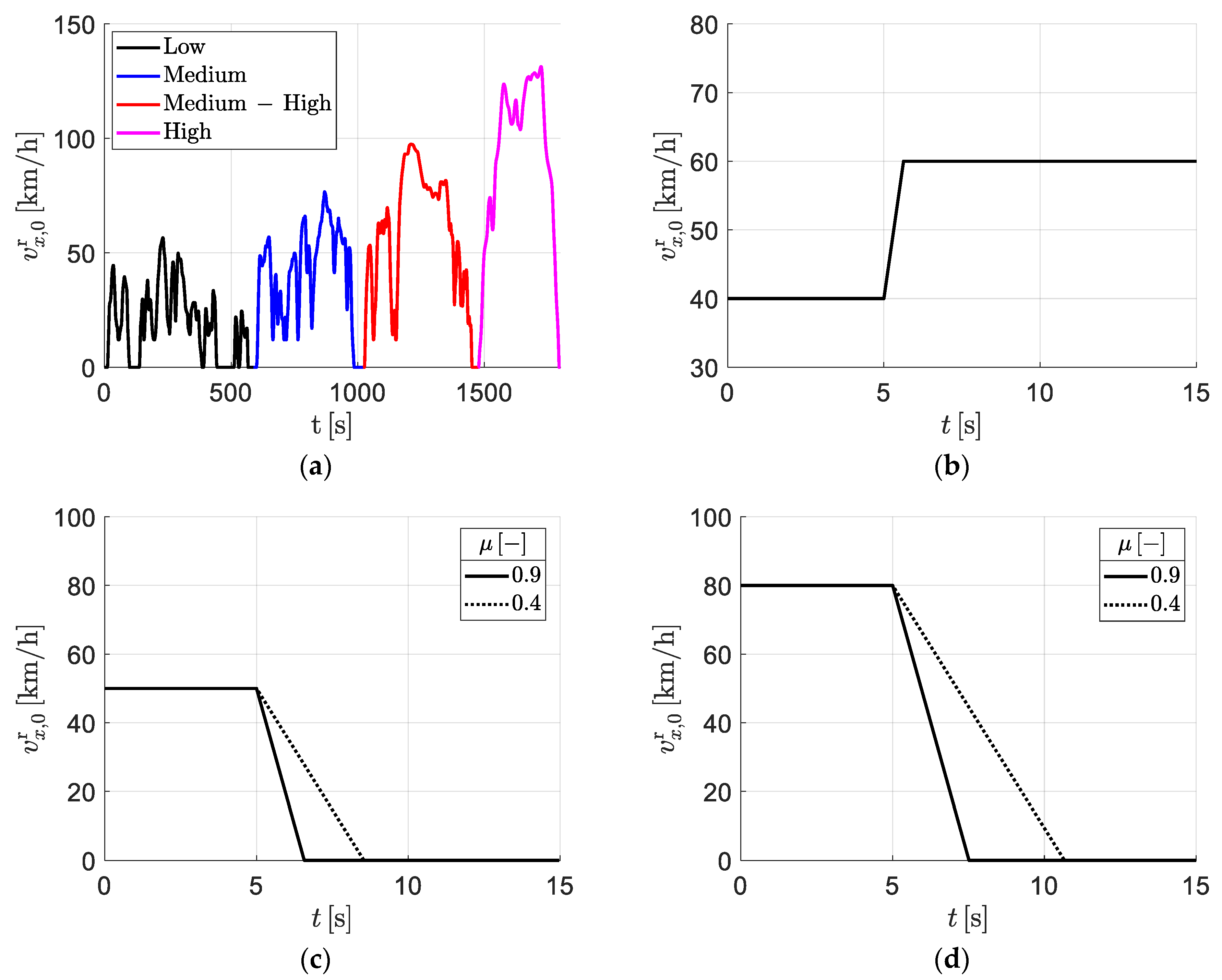
The WLTP Class 3 cycle is adopted as a reference manoeuvre to represent realistic driving conditions over a broad speed range. The cycle includes low-, medium-, medium–high, high-speed phases, reaching a maximum speed of approximately $131$ km/h and covering about $23$ km over $1800$ s. Its highly dynamic profile, characterised by frequent accelerations and decelerations, makes it suitable for assessing energy consumption and overall closed-loop performance. Simulations are carried out assuming a nominal road friction coefficient $\mu =0.9$.

4.1.2. Emergency Braking

A full-stop emergency braking manoeuvre is introduced to assess safety-critical behaviour. The leader vehicle decelerates from an initial speed v_0 to standstill using the maximum achievable deceleration $a_{x,\mathrm{m}\mathrm{a}\mathrm{x}}=\mu g$. Two initial speeds are considered, $v\_0=80$ km/h and $v_0=50$ km/h, under both high-friction ($\mu =0.9$) and low-friction ($\mu =0.4$) conditions.

4.1.3. Acceleration

A mild acceleration test is defined to evaluate transient comfort and tracking performance. The leader speed is increased from $v_0=40 \mathrm{km}/\mathrm{h}$ to $v_1=50 \mathrm{km}/\mathrm{h}$ using a ramp profile, with $\mu =0.9$. This manoeuvre is selected to excite platoon dynamics, enabling a systematic assessment of controller sensitivity across the parameter space. The use of a saturated ramp provides a more dynamic and demanding input than smoother driving profiles, making the effects of controller calibration on longitudinal dynamics and comfort clearly observable and allowing for a consistent comparison between configurations.

Figure 3 shows the time histories of the speed reference profiles during the driving scenarios used for calibration: Figure 3a shows the WLTP driving cycle, Figure 3b the acceleration manoeuvre, and Figure 3c,d the emergency braking manoeuvres.

4.2. Structure of the Weight Matrices

This section presents the rationale adopted for defining the structure of the LQR weighting matrices. The input weighting matrix $\mathit{R}$ is assumed to be diagonal, with identical diagonal entries, in accordance with the assumption of a homogeneous platoon:

$$\mathit{R}=R_0\cdot \mathrm{d}\mathrm{i}\mathrm{a}\mathrm{g}(1,\dots ,1)$$

(41)

The state weighting matrix $\mathit{Q}$ is defined on the basis of a preliminary sensitivity analysis by introducing the weights $w_{e_d,i}$, $w_{e_v,i}$, and $w_{\int e_d,i}$, associated with the distance error, speed error, and integral of the distance error, respectively:

$$\mathit{Q}=\mathrm{d}\mathrm{i}\mathrm{a}\mathrm{g}(w_{e_{d,1}},w_{v,1},w_{d,2},w_{v,2},w_{\int e_{d,1}},{\mathrm{w}}_{\int e_{d,2}})$$

(42)

In order to define the structure of the state weighting matrix adopted throughout the calibration maps, a sensitivity analysis is carried out on the minimum damping ratio $\zeta$ of the closed-loop system.

A design region $0.7\le {\zeta }_{\mathrm{m}\mathrm{i}\mathrm{n}}\le 0.8$ was selected, as it corresponds to a favourable trade-off within the LQR tuning framework, where the weighting matrices implicitly balance state regulation and control effort. In this range, overshoot is effectively reduced while maintaining a sufficiently fast response, without driving the solution toward overly conservative dynamics or excessive control action.

Three sensitivity studies are considered:

• Two-dimensional maps in the $\left(w_{e_d},w_{e_v}\right)$ plane for fixed $w_{\int e_d}$;
• Two-dimensional maps in the $\left(w_{e_d},w_{\int e_d}\right)$ plane for fixed $w_{e_v}$;
• Two-dimensional maps in the $\left(w_{e_d},w_{e_v}\right)$ plane for fixed $R_0$.

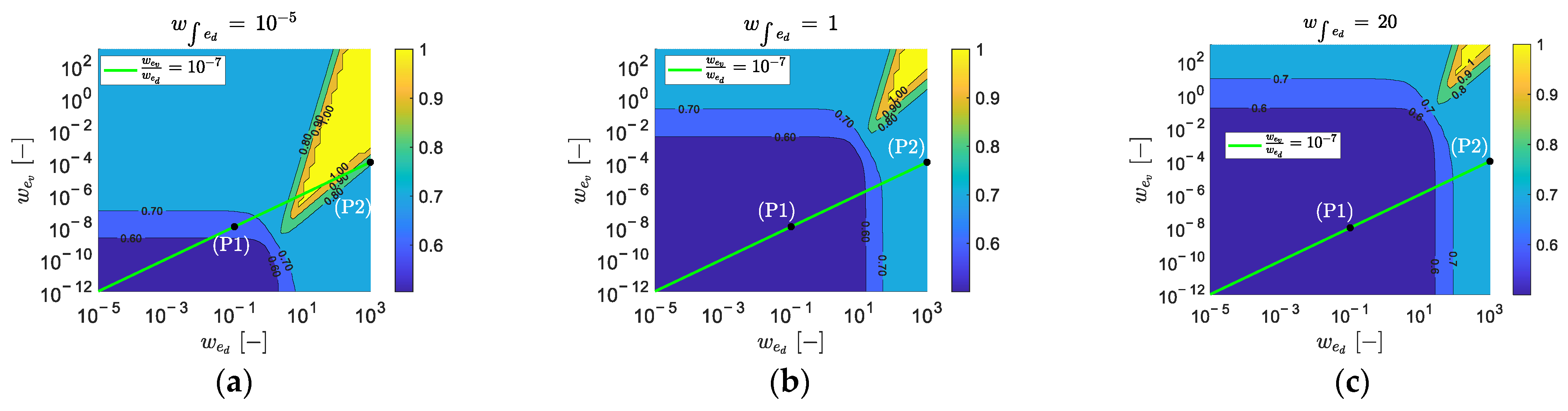
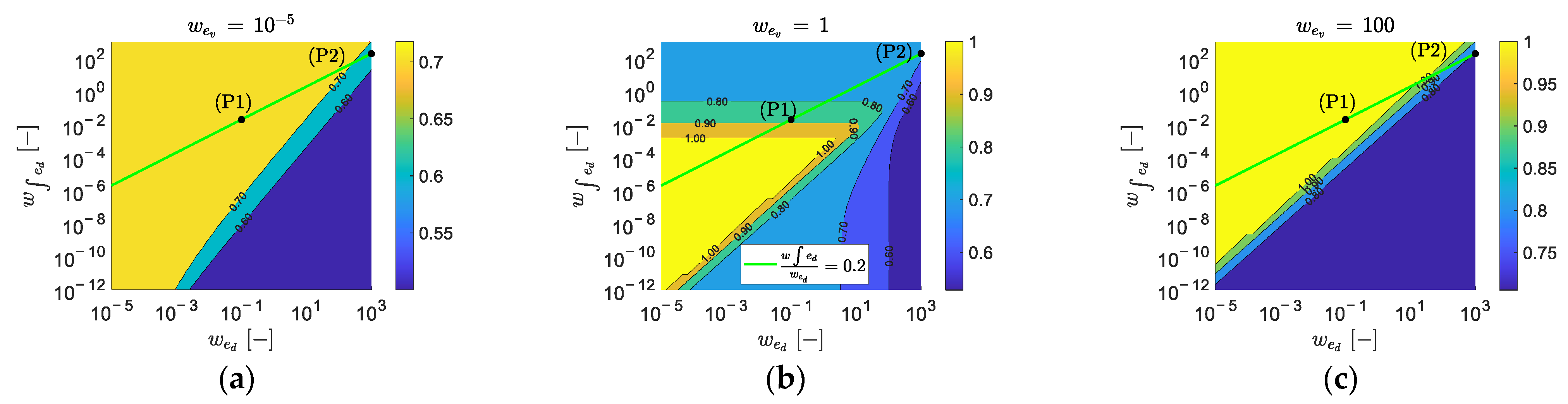
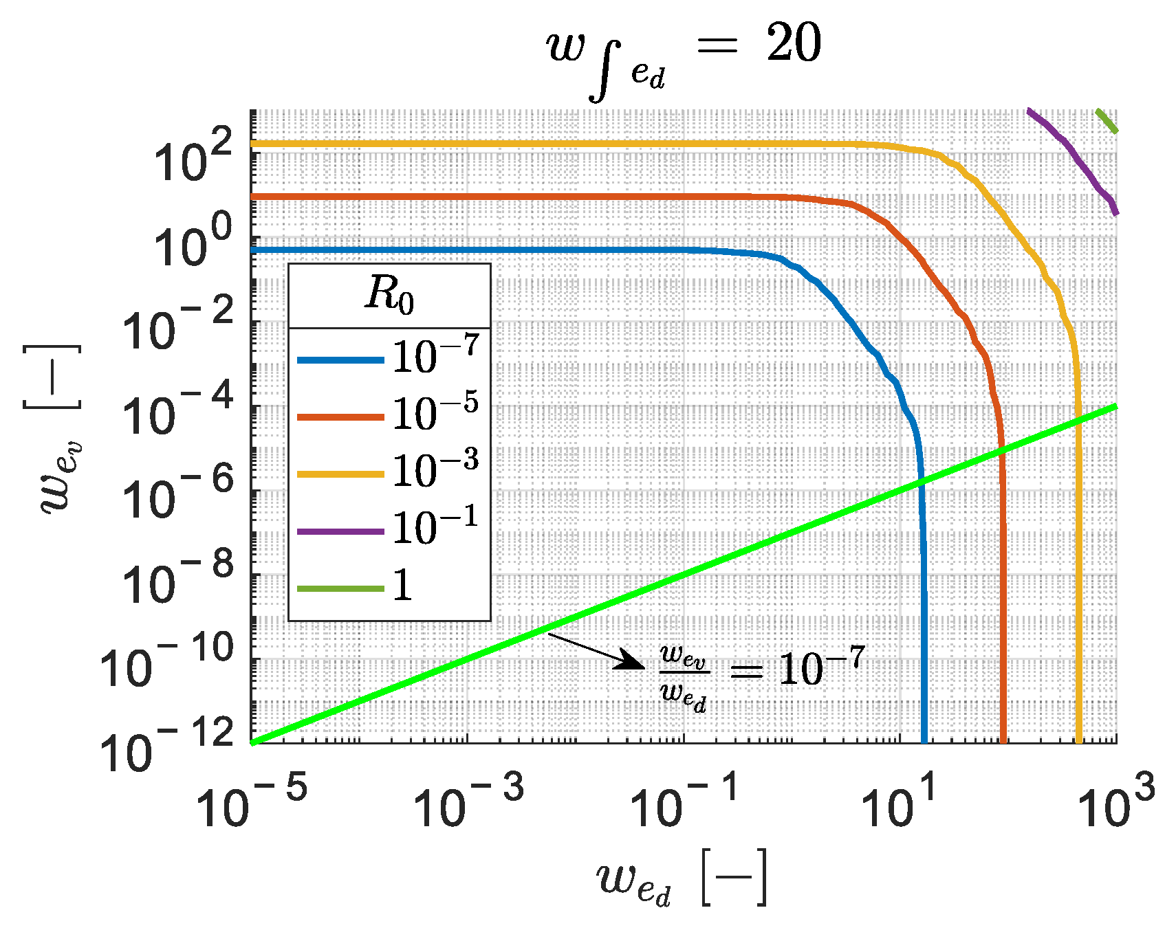
Figure 4 shows the two-dimensional maps of the minimum damping ratio evaluated over the range of $w_{e_d},w_{e_v}\in [{10}^{-3},{10}^3]$, for three values of the integral weight $w_{\int e_d}$, namely ${10}^{-5}$, $1$, and $20$, with $R_0={10}^{-5}$. The results indicate that the requirement $0.7\le {\zeta }_{min}\le 0.8$ is satisfied in two regions, top left and bottom right corners, with comparable iso-damping characteristics: one corresponding to $w_{e_d}\gg w_{e_v}$, where distance tracking is prioritised, and the other to $w_{e_v}\gg w_{e_d}$, where speed tracking becomes dominant. Since both regions satisfy the damping-ratio requirement, the final selection is based on the control objective of the proposed CACC strategy. In particular, the distance-tracking-oriented region is retained, as preserving accurate inter-vehicle spacing is considered more relevant than prioritizing speed tracking alone.

To reduce the dimensionality of the design problem while retaining sufficient flexibility to explore the design space, a constraint relating the two weights is introduced. This constraint defines a straight line in the design space (shown in green), which is further restricted to the segment between points P1 and P2 to remain within the preferred region. A subset of the design space corresponding to a constant weight ratio of $w_{e_v}/w_{e_d}={10}^{-7}$, represented by the green line in Figure 4, is therefore selected. This ratio is retained because it lies within the distance-tracking-oriented region satisfying the prescribed damping-ratio range. It therefore prioritises inter-vehicle distance regulation, which is the most relevant tracking objective for collision avoidance, while preserving a fixed balance between distance and speed tracking. Comparison of the three graphs in Figure 4 shows that a ratio of ${10}^{-7}$ provides an adequate minimum damping factor over the full range of integral-term weight $w_{\int e_d}$ considered.

The second analysis, namely the two-dimensional map in the $\left(w_{e_d},w_{\int e_d}\right)$ plane, is reported in Figure 5 and allows the effect of the integral distance-error weight on the damping ratio to be further investigated. The results support the selected structure, in which the integral contribution is constrained with respect to the proportional distance term by a factor of $0.2$. This value preserves the prescribed damping-ratio range along segment P1P2 while retaining integral action for distance-error compensation.

Finally, the third sensitivity analysis, shown in Figure 6, illustrates the effect of the control weighting factor $R_0$ in the $\left(w_{e_d},w_{e_v}\right)$ plane. Specifically, it identifies the combinations of parameters that satisfy the lower bound of the desired damping ratio range, i.e., $\zeta =0.7$. As $R_0$ increases, the control effort is more heavily penalised in the LQR cost function, causing the boundary to shift toward the top-right corner of the plot.

Accordingly, the ratios ${10}^{-7}$ for the speed-error weights and $1/5$ for the integral-state weights are imposed as constraints in the subsequent sensitivity analysis, as they provide a satisfactory trade-off between the competing requirements of distance tracking, closed-loop damping performance, and control effort. Under these assumptions, the calibration of the weighting matrix $\mathit{Q}$ reduces to the exploration of a single parameter, namely $Q_0$, within the range defined by the segment P1P2, as expressed by:

$$\mathit{Q}=Q_0\cdot \mathrm{d}\mathrm{i}\mathrm{a}\mathrm{g}({1, 10}^{-7},{1, 10}^{-7}, {\displaystyle \frac{1}{5}}, {\displaystyle \frac{1}{5}})$$

(43)

4.3. Parameter Space Definition

Once the structure of the matrix $\mathit{Q}$ and $\mathit{R}$ are defined, the performance maps are generated by exploring two sets of tuning parameters defined over two-dimensional grids:

• ${\Gamma }_{Q,R}=\left(Q_0,R_0\right)$, defined over a grid of 30 × 19, points;
• ${\Gamma }_{t_{h,R}}=\left(t_{h,0}{R}_0\right)$, defined over a grid of 17 × 21, points.

Table 3. Minimum and maximum values of the space parameter set $t_{h,0},R_0,Q_0.$

Parameter	Symbol	Value	Unit
Minimum time headway	$t_{h,0}^{min}$	$1$	[s]
Maximum time headway	$t_{h,0}^{max}$	$5$	[s]
Minimum control weight	$R_0^{min}$	${10}^{-7}$	[-]
Maximum control weight	$R_0^{max}$	${10}^{-2}$	[-]
Minimum state weight	$Q_0^{min}$	${10}^{-1}$	[-]
Maximum state weight	$Q_0^{max}$	${10}^3$	[-]

illustrates the minimum and maximum values used for the grid of ${\Gamma }_{Q,R}$ and ${\Gamma }_{t_h,R}$ sets.

The evaluation of each KPI is associated with specific driving scenarios, selected to stress the relevant aspects of platoon dynamics.

Table 4. Case studies analysed for assessing the performance of the CACC over the calibration sets. ✓ indicates that the KPI is evaluated from the specific manoeuvre, while × indicates that is not included.

KPI Maps	Driving Cycle	Braking	Acceleration
$k_{\mathrm{B}\mathrm{S}\mathrm{I}}$	✓	✓	×
$k_{\mathrm{R}\mathrm{M}\mathrm{S}\left(a_x\right)}$	×	×	✓
$k_{\mathrm{E}\mathrm{S}}$	✓	×	×

summarises the mapping between the KPIs and the considered manoeuvres, including the WLTP Class 3 cycle, emergency braking, acceleration tests. Safety metric is evaluated under critical conditions, while comfort and energy indicators are computed under representative transient and realistic driving profiles.

Table 5. Platooning nominal conditions set for the numerical simulations.

Manoeuvre	${\mathit{v}}_{\mathit{x},\mathbf{n}}$ [km/h]	${\mathit{d}}_{\mathbf{n}}$ [m]	${\mathit{d}}_0$ [m]
WLTP Class 3	$80$	$36.3$	$3$
Emergency braking	$80$	$36.3$	$3$
Acceleration	$80$	$36.3$	$3$

summarises the nominal conditions used for the numerical simulations for the sensitivity analysis.

5. Results and Discussion

5.1. Sensitivity Q-R

In this section, the parameter set ${\Gamma }_{Q,R}$ is explored to generate 2D performance maps as functions of the weighting parameters $Q_0$ and $R_0$. For all the maps presented in the following sections, the time headway is fixed at $t_h=1.5$ s.

5.1.1. $k_{\mathrm{B}\mathrm{S}\mathrm{I}}$ Map

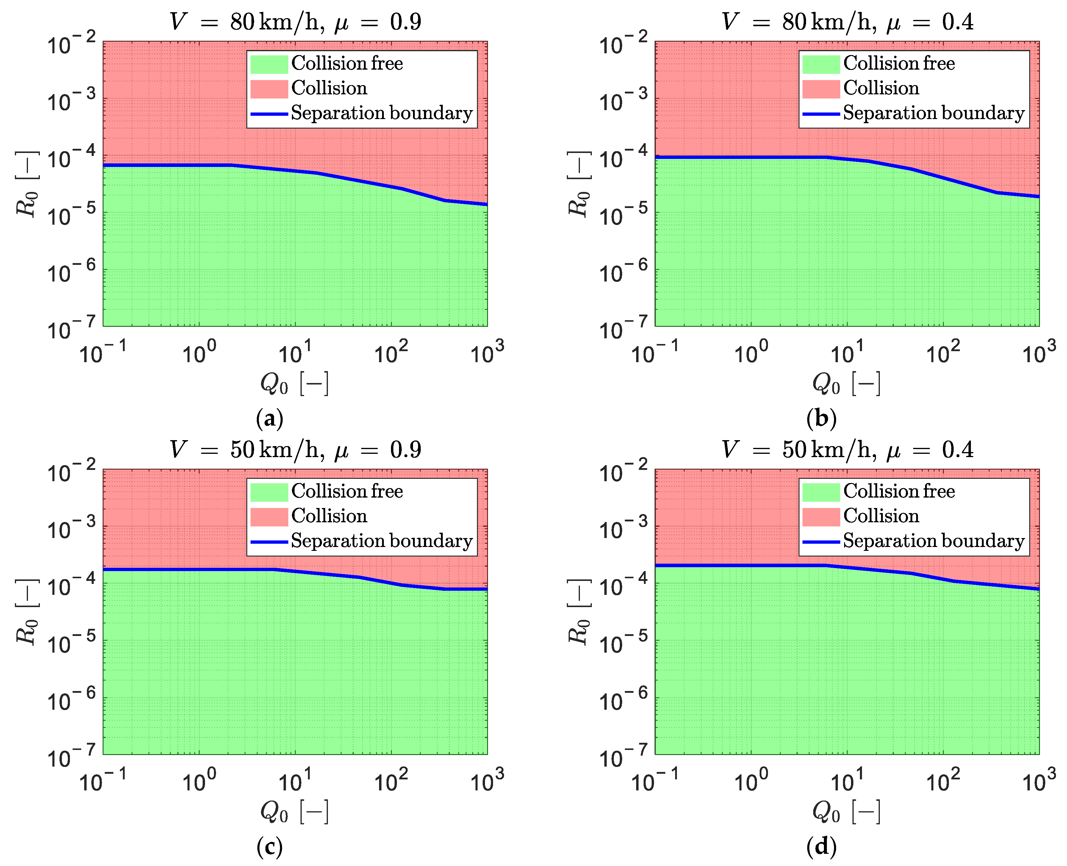
Figure 7 shows the distribution of the binary safety indicator $k_{\mathrm{B}\mathrm{S}\mathrm{I}}$ over the $(Q_0,R_0)$ grid, obtained from the emergency braking maneuver. The map distinctly separates safe and unsafe controller configurations: the green region corresponds to collision-free stopping conditions, whereas the red region identifies parameter combinations that lead to rear-end collisions during emergency braking. The blue curve marks the nominal separation boundary between the two regions. The results indicate that safety is primarily influenced by the control effort weight $R_0$, while the effect of the state weight $Q_0$ is comparatively limited. In particular, the safe region is achieved for values of $R_0$ below approximately ${10}^{-4}$, whereas $Q_0$ can be varied over a wide range without significantly affecting collision avoidance. Moreover, the extent of the safe region increases at lower initial speeds, while the influence of the friction coefficient remains relatively limited within the range considered. A slight upward shift of the boundary line is observed when moving from high to low friction conditions, more noticeably at 80 km/h.

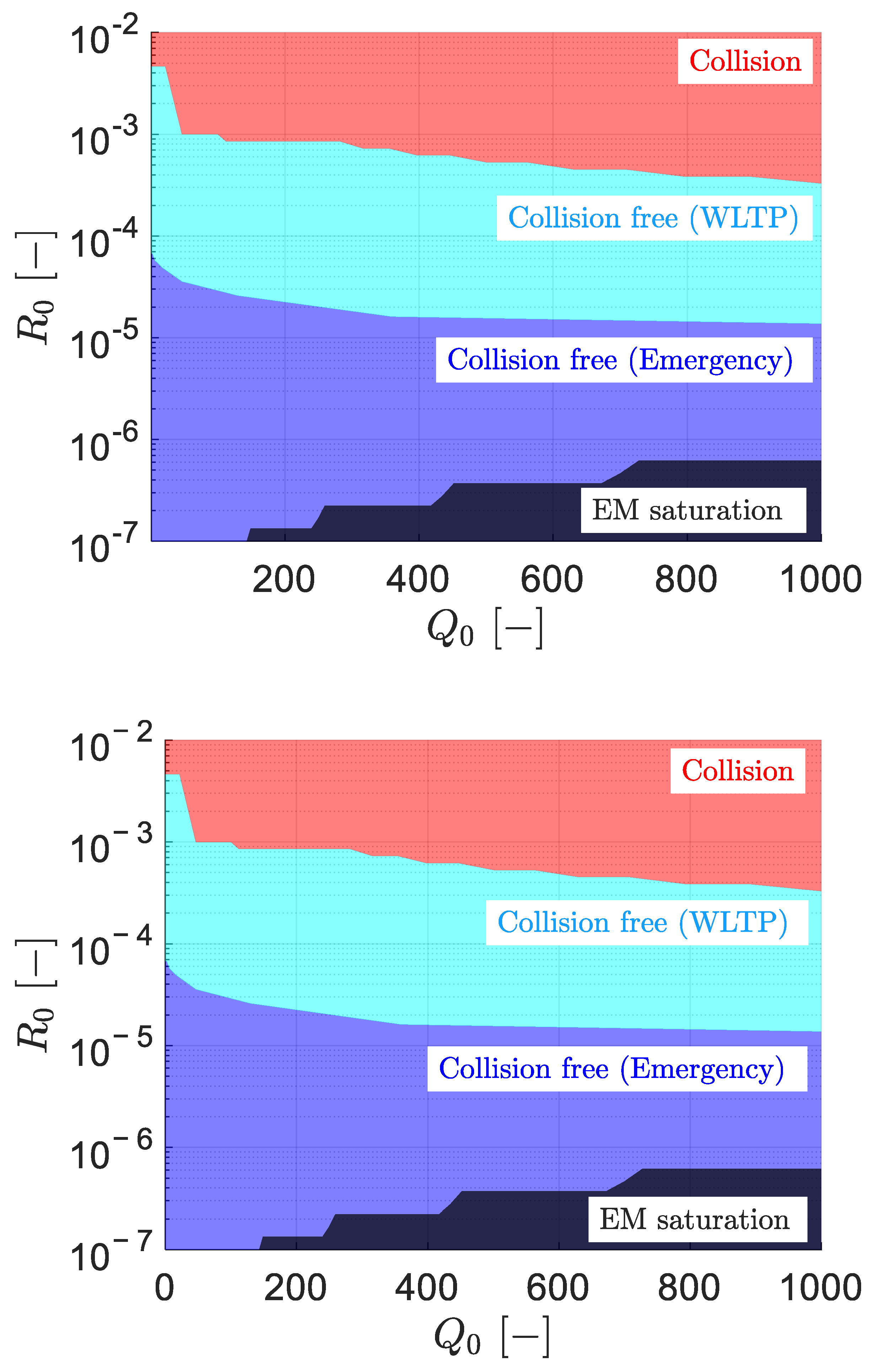
The safety KPI is also evaluated over the WLTP driving cycle, where braking demands are less severe and more representative of nominal driving conditions. The comparison between the collision-free regions obtained from the emergency braking test and the WLTP cycle is shown in Figure 8. The cyan region represents the collision-free domain under WLTP conditions, while the blue region corresponds to the more restrictive collision-free region identified from the emergency braking scenario. Results show that, under the WLTP scenario, a wider range of $R_0$ values ensure collision-free operation. This indicates that less conservative control effort penalties can be adopted while maintaining safe inter-vehicle distances, potentially improving comfort and energy performance. In contrast, the influence of $Q_0$ on safety boundaries is more pronounced at lower values, whereas at higher values it follows a monotonically decreasing, approximately linear trend with a shallow slope. These findings suggest that different tuning levels, ranging from more aggressive to more comfort-oriented configurations, can be selected according to the driving context without compromising safety. Finally, the dark shaded region in the map identifies parameter combinations that lead to saturation of the electric motor. This region should be avoided, as actuator saturation may degrade tracking performance and limit the effectiveness of the control action.

5.1.2. $k_{\mathrm{R}\mathrm{M}\mathrm{S}\left(a_x\right)}$ Map

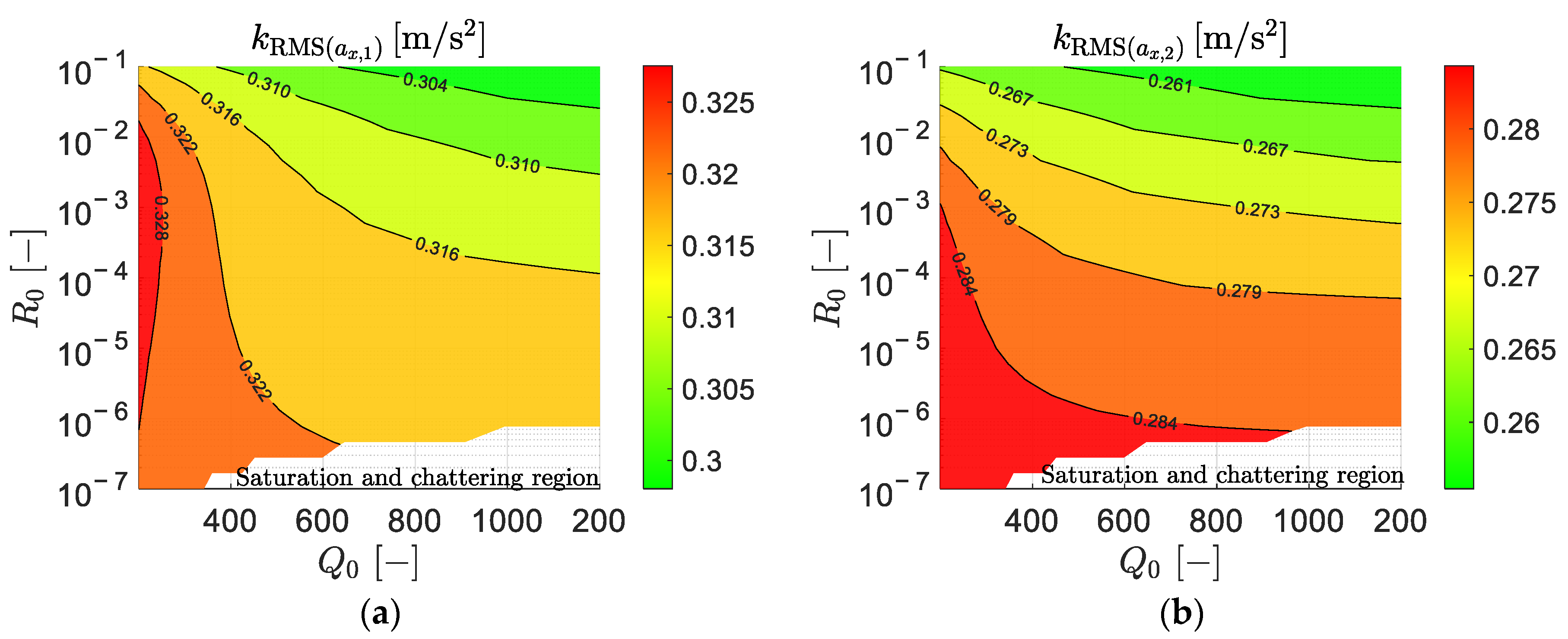
Figure 9 illustrates the comfort performance in terms of RMS longitudinal acceleration for follower 1 and follower 2 during the acceleration manoeuvre. The results show a progressive reduction in comfort as $R_0$ decreases, due to the more aggressive control action, which leads to faster actuator responses during vehicle acceleration. Comfort levels are consistently better for follower 2, because of the attenuation of longitudinal dynamics along the platoon, already observed in the safety analysis. The inclusion of physical constraints, such as tyre–road friction limits and actuator saturation, leads to the identification of specific regions in the controller parameter space that must be excluded, as they generate control chattering, as indicated in Figure 9.

5.1.3. $k_{\mathrm{E}\mathrm{S}}$ Map

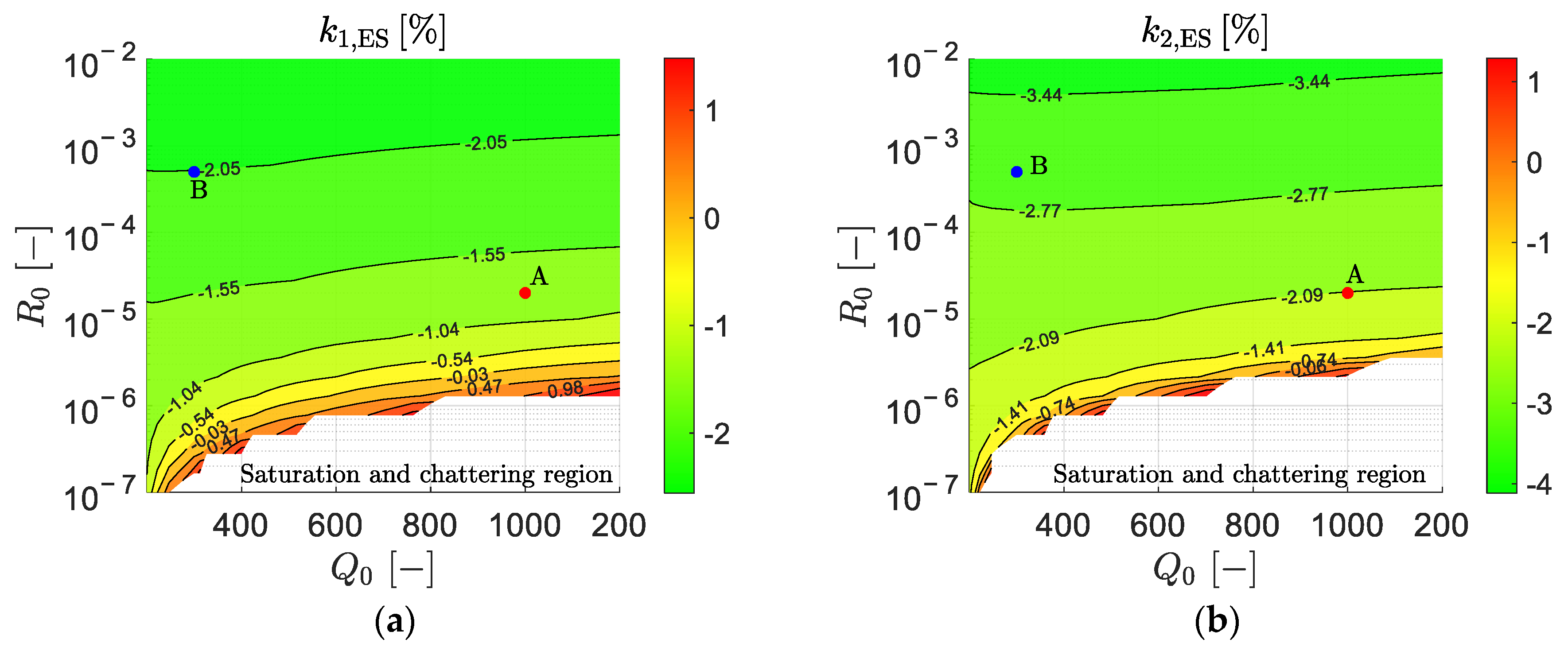
Figure 10 presents the 2D maps of the energy saving obtained from the WLTP driving cycle. To isolate the benefits of platoon driving in terms of dynamics performance, aerodynamic drag reduction maps for the following vehicles was disabled. Both followers feature a reduction in electric energy consumption compared to the isolated case, due to the speed smoothing in the velocity profile. The effect of the control weight $R_0$ slightly impact the energy saving in both followers; however, the smallest reduction occurs for small $R_0$ and large $Q_0$ values. This behaviour is associated with more responsive control actions that allow the followers to maintain shorter inter-vehicle distances, particularly at higher speeds. A further reduction in the $k_{\mathrm{E}\mathrm{S}}$ is observed for the second follower over the entire parameter range, confirming the expected energy benefit along the platoon.

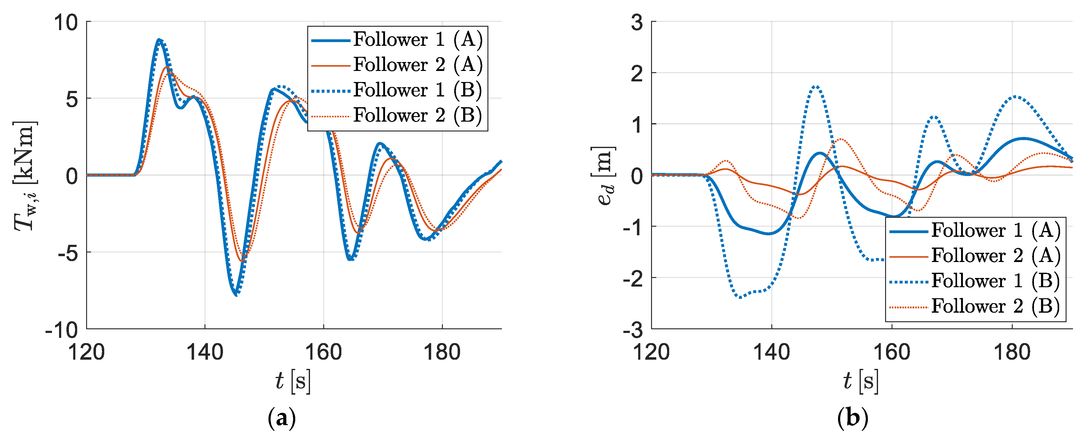
To better highlight the effect of the weights $R_0$ and $Q_0$, two cases (A and B) were considered, as indicated in Figure 10. Figure 11 shows the wheel torque (Figure 11a) and inter-vehicle distance error (Figure 11b) over a segment of the WLTP driving cycle for follower 1 (blue curves) and follower 2 (orange curves). The results show that the smoother torque profile obtained in Case B leads to reduced energy consumption; conversely, Case A provides improved tracking of the preceding vehicles, as evidenced by the inter-vehicle distance error.

5.2. $t_h-R$ Map

To further investigate the interaction between controller tuning and spacing policy design, performance maps were generated in the ${(t}_{h,0}-R_0)$ plane. The parameter $Q_0$ was fixed to 100, based on the previous $Q-R$ analysis.

5.2.1. $k_{\mathrm{B}\mathrm{S}\mathrm{I}}$ Map

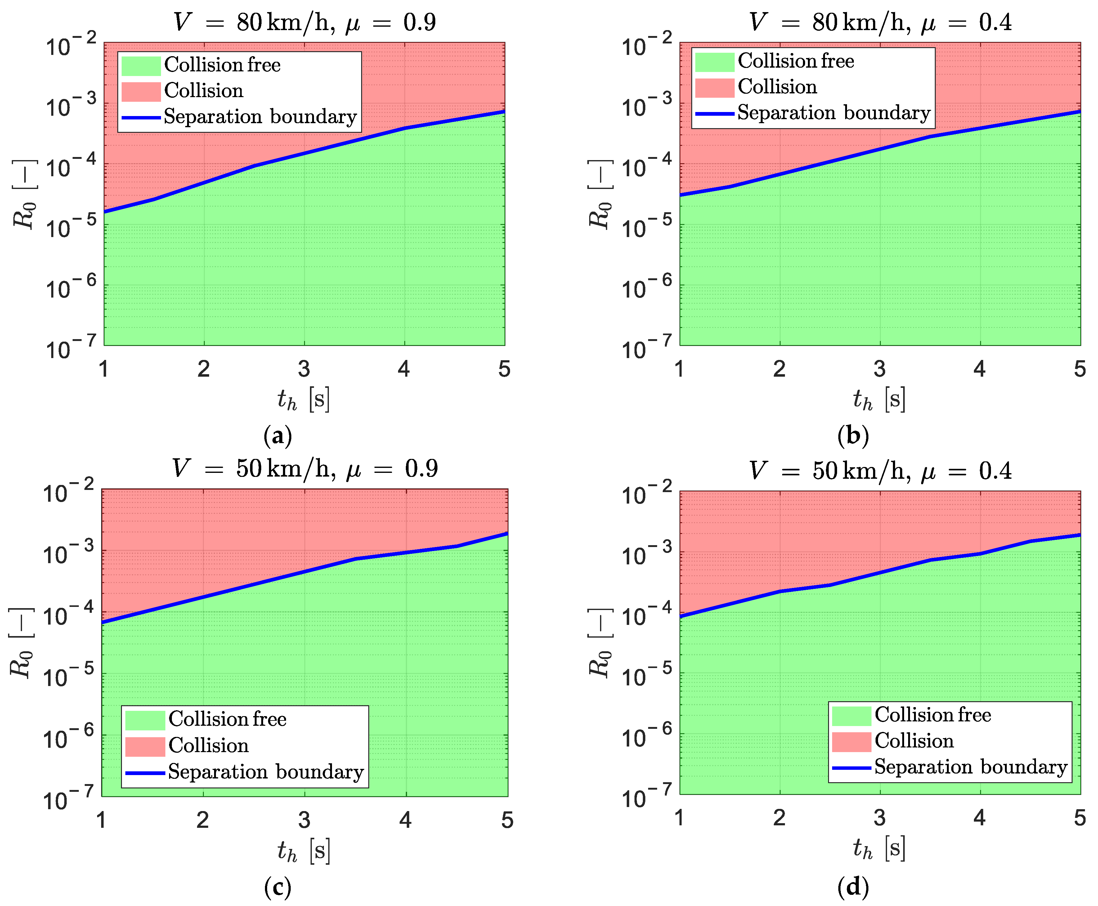
Figure 12 shows the $k_{\mathrm{B}\mathrm{S}\mathrm{I}}$ maps in the ${(t}_{h,0}-R_0)$ plane, highlighting the safe and unsafe regions over the explored parameter ranges. At fixed $R_0$, the collision-free region expands as the time headway increases, as expected, since larger $t_h$ values correspond to greater inter-vehicle distances. Conversely, for a fixed $t_h$, the collision-free region increases as $R_{0 }$ decreases, indicating that more aggressive control actions improve collision avoidance during emergency braking. The safety boundary exhibits an approximately linear trend with respect to both the time headway and the control effort weight $R_0$. Increasing the initial speed $v_{x,0}$ reduces the feasible collision-free region, requiring higher control effort to ensure collision-free braking within the platoon. In contrast, the influence of road friction is less pronounced, with noticeable differences mainly for time headway values below $2 \mathrm{s}$.

5.2.2. $k_{\mathrm{R}\mathrm{M}\mathrm{S}\left(a_x\right)}$ Map

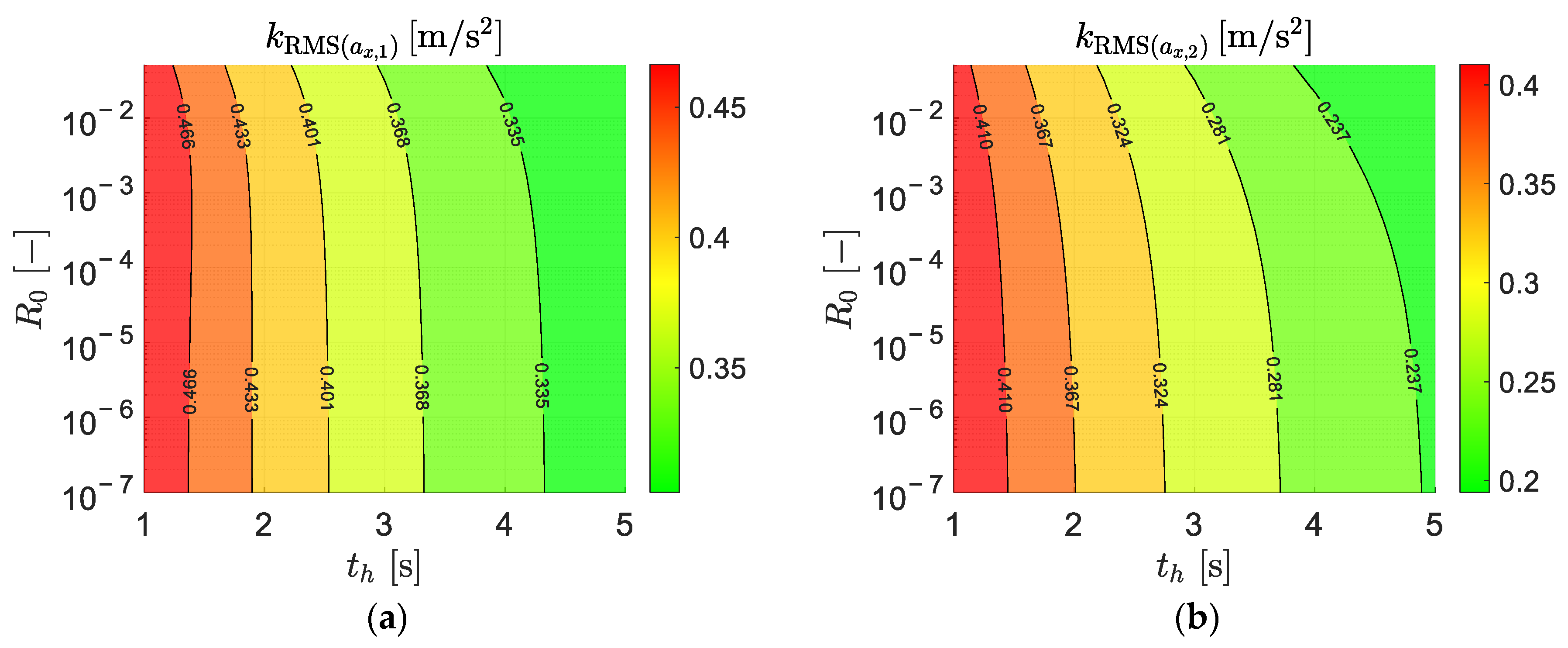
Figure 13 shows the maps of the RMS longitudinal acceleration for follower 1 and follower 2 obtained from the acceleration test. For both vehicles, the RMS values decrease as the time headway increases, while the influence of $R_0$ within the considered range appears less pronounced. Smaller time headways, corresponding to reduced inter-vehicle gaps, result in more aggressive control actions and, consequently, slightly higher acceleration levels, which may reduce ride comfort. Nevertheless, all values remain within the comfort limits.

5.2.3. $k_{\mathrm{E}\mathrm{S}}$ Map

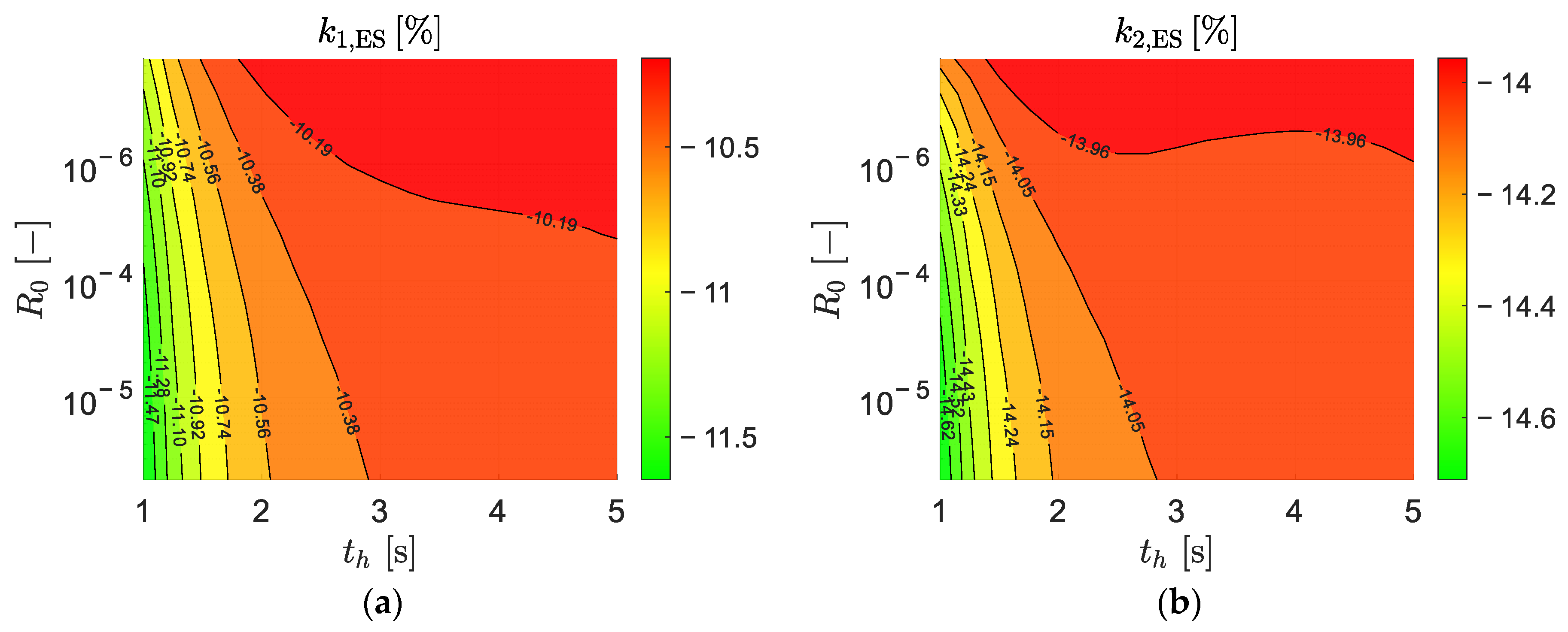
Figure 14 shows the AEC maps for follower 1 and follower 2 obtained from simulations over the WLTP Class 3 driving cycle. For both vehicles, the results indicate an increase in average energy consumption as the time headway increases. This trend is more pronounced for follower 2, which consistently exhibits lower energy consumption than follower 1 for a given time headway. The observed energy savings at smaller time headways are consistent with the reduction in aerodynamic drag associated with closer inter-vehicle spacing, as captured by the nonlinear drag coefficient scaling introduced in Equation (3).

5.3. Controller Calibration Under Off-Nominal Model Parameters

The map-based approach is extended in this section to the calibration of the LQR weighting matrices under off-nominal model parameters. In particular, collision-avoidance maps are re-evaluated considering vehicle mass variations of $\pm 20\%$ relative to the nominal mass $m_{nom}$, to identify the corresponding uncertainty band of the separation boundary during the emergency-braking test. In addition, the sensitivity of the calibration maps to rolling resistance and aerodynamic drag is investigated by considering variations of $\pm 20\%$ with respect to the nominal rolling-resistance coefficient $f_{0,nom}$ and the nominal drag coefficient, respectively.

5.3.1. Mass Uncertainty

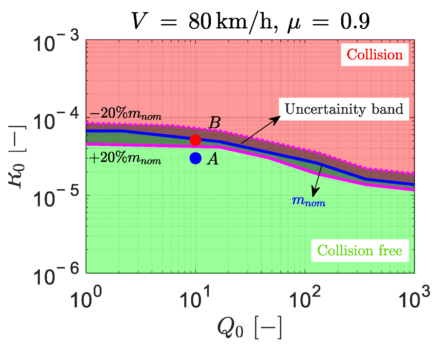
Figure 15 shows collision map obtained by considering a mass variability of ±20% with respect to the nominal value $m_{\mathrm{n}\mathrm{o}\mathrm{m}}$. It is worth highlighting the reduction in the collision-free zone, whose boundaries are indicated in solid purple for the case in which both followers have a mass of $+20$% relative to $m_{nom}$, and in dotted purple for the case with $-20$% relative to $m_{nom}$. All the intermediated cases lie between the two separation-boundary curves.

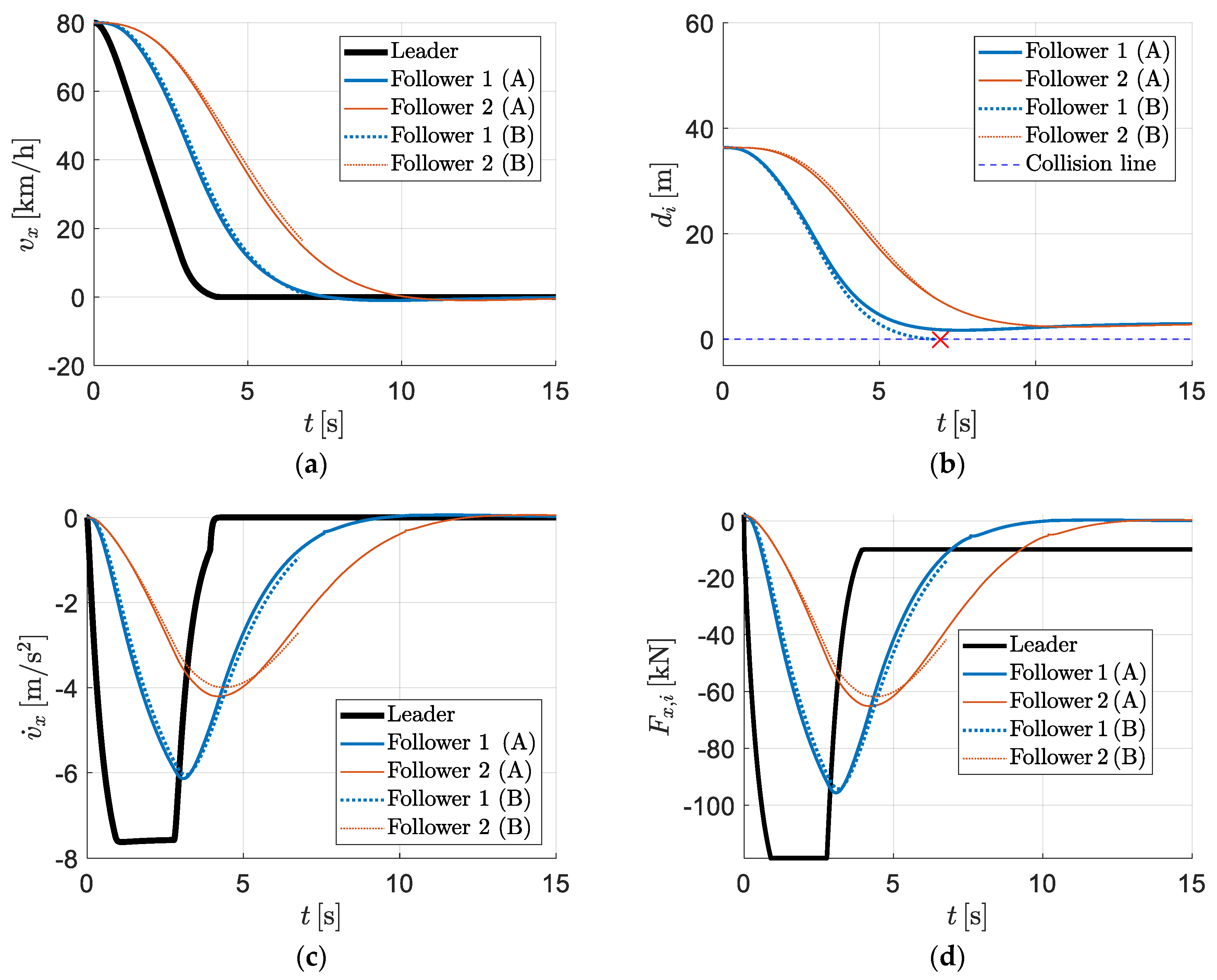
Figure 16 illustrates the time histories of the three MDVs during an emergency braking manoeuvre on a high-friction road surface, starting from 80 km/h, for cases A and B shown in Figure 15: speeds (Figure 16a), inter-vehicle distances (Figure 16b), accelerations (Figure 16c), and longitudinal forces (Figure 16d). In configuration A, Followers 1 and 2 accurately reproduce the speed profile of the leader, which decelerates by exploiting the maximum available friction, thereby avoiding collisions while maintaining the minimum admissible inter-vehicle distance. In contrast, configuration B results in a collision between Follower 1 and the lead vehicle. In conclusion, uncertainty in the mass of the vehicles within the platoon requires the adoption of a more conservative calibration than the nominal tuning to prevent collisions. This highlights the practical relevance of the grey region associated with parametric uncertainty.

5.3.2. Rolling Resistance Uncertainty

No appreciable variation is observed in the collision maps over the explored $\mathit{Q}$-$\mathit{R}$ calibration space when rolling resistance is varied. The results are not included in the paper because it is practically coincident with the ones reported in Figure 7. Therefore, within the considered range, rolling resistance does not represent a critical factor for collision avoidance.

The main effect of rolling resistance is instead reflected in the energy performance. For this reason, the $k_{ES}$ indicator is used to compare the platooning performance under different rolling-resistance levels.

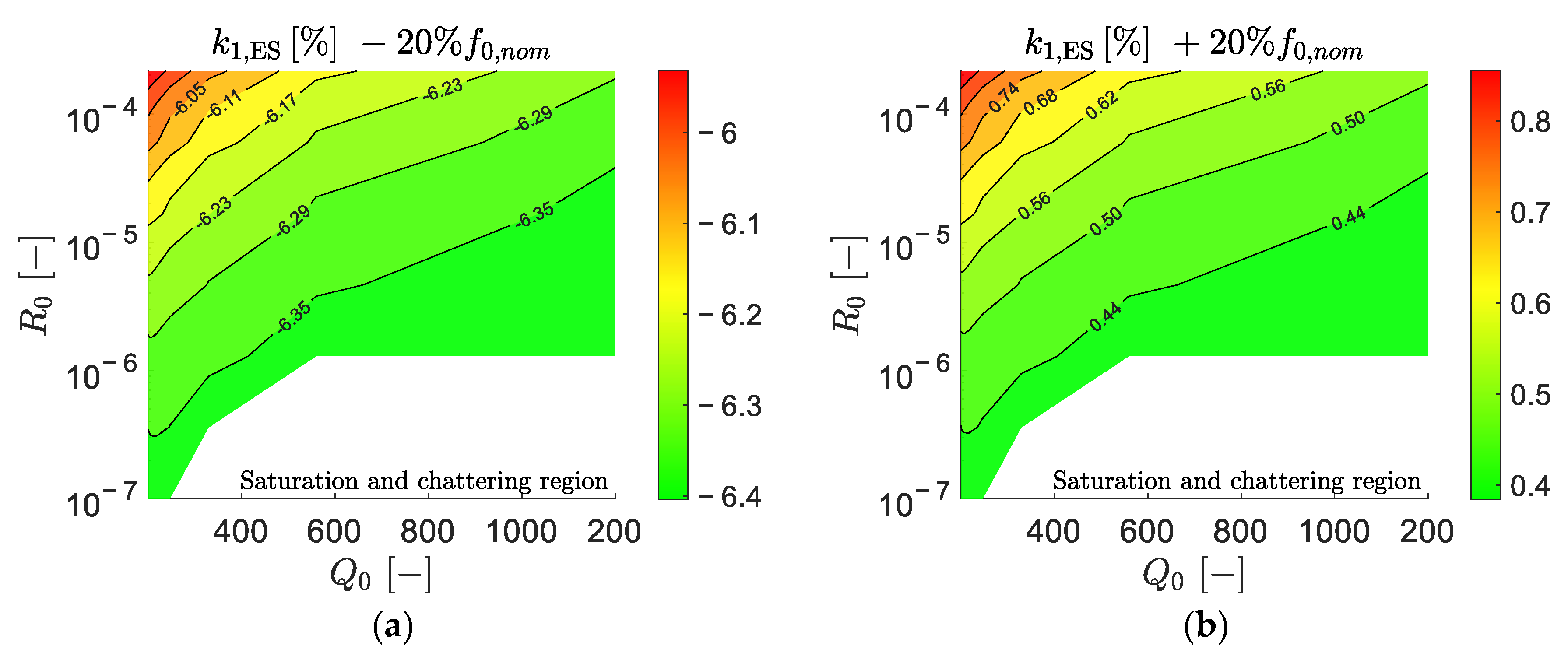
Figure 17 shows the energy-saving results for Follower 1 under a reduced rolling resistance, equal to $-20\% f_{0,\mathrm{n}\mathrm{o}\mathrm{m}}$ (Figure 17a), and an increased rolling resistance, equal to $+20\% f_{0,\mathrm{n}\mathrm{o}\mathrm{m}}$ (Figure 17b), with respect to the corresponding reference value of the isolated-vehicle case (with $f_0=f_{0,nom})$. As expected, a reduction in rolling resistance leads to increased energy savings, while a slightly increase is appreciated for the case with $+20\% f_{0,\mathrm{n}\mathrm{o}\mathrm{m}}$. Nevertheless, the maps in Figure 17 exhibit very similar qualitative trends, indicating that the relationship between energy consumption and controller parameter calibration is largely unaffected by variations in rolling resistance.

5.3.3. Drag Coefficient

Similar considerations apply to variations in the nominal drag coefficient $c_{x,0,\mathrm{n}\mathrm{o}\mathrm{m}}$. No appreciable differences are observed in the collision maps across the explored calibration space; therefore, these results are omitted as they closely match those shown in Figure 7.

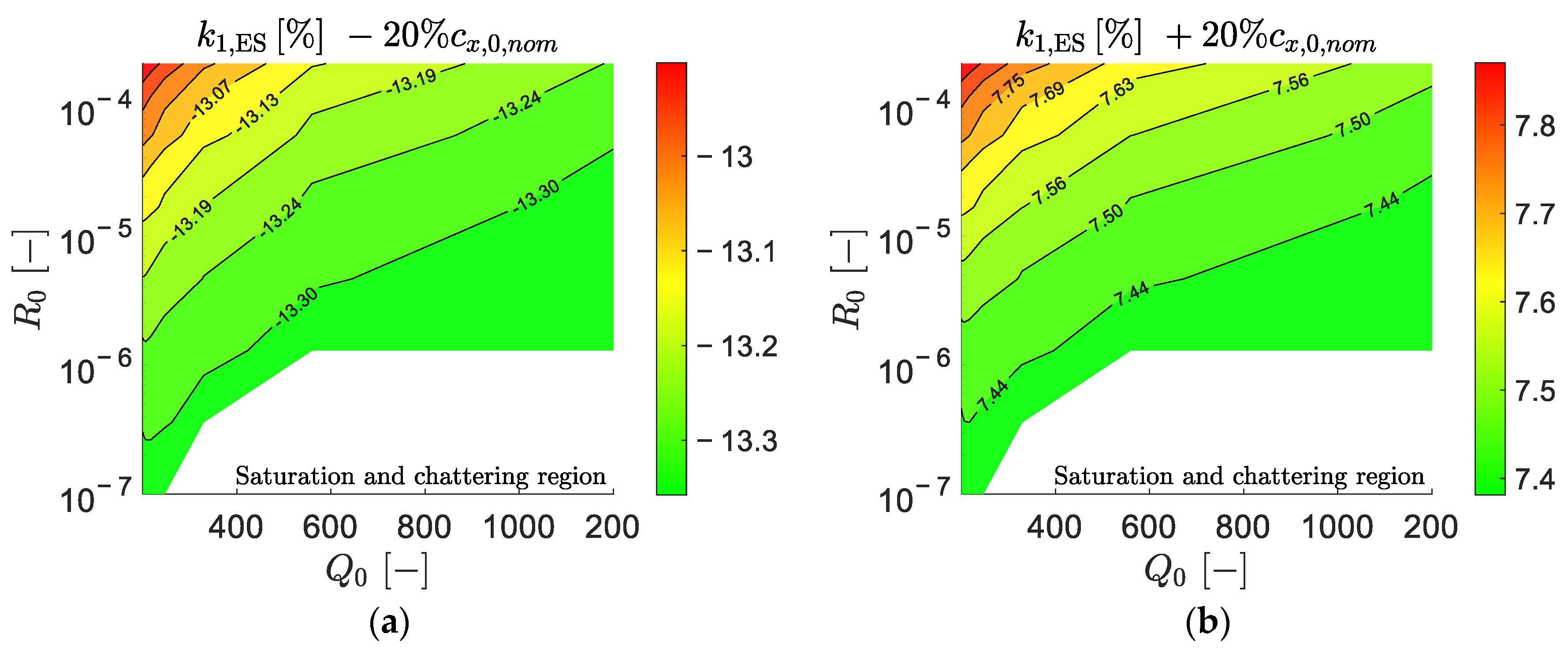
Their main influence is instead reflected in the energy performance. Figure 18 shows the energy-saving map $k_{ES }$ for Follower 1 under off-nominal values of the drag coefficient during platoon driving over the WLTP Class 3 cycle.

As expected, reducing the aerodynamic drag coefficient increases energy savings. However, the maps in Figure 18 display consistent qualitative trends, suggesting that the relationship between energy consumption and controller parameter calibration is largely insensitive to variations in the aerodynamic drag model parameters.

5.4. Practical Implementation of the Map-Based Tuning

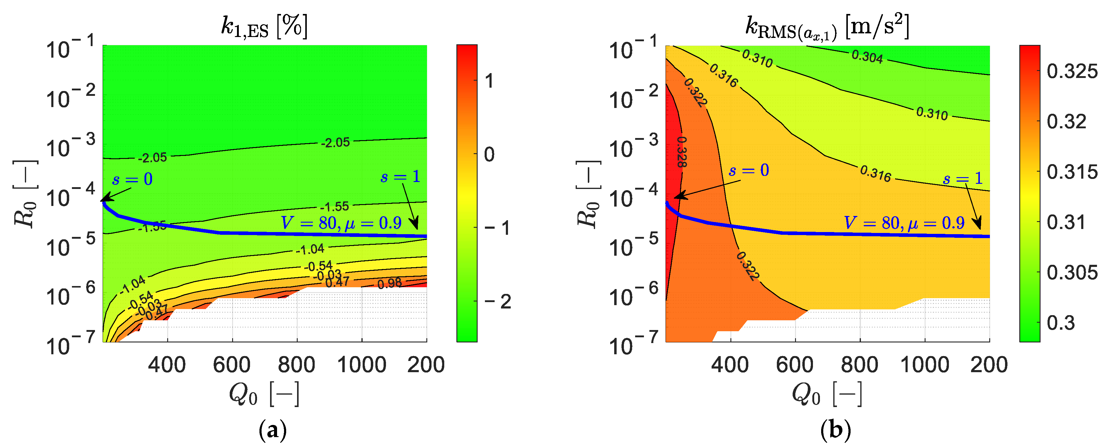
This section illustrates a practical implementation of the proposed map-based tuning approach for the offline calibration of the controller. In this framework, the calibration maps are used as an offline database for the ECCU. The database is generated for a discrete set of representative operating conditions, defined by vehicle speed $v$ and tyre–road friction coefficient $\mu$. For each $(v,\mu )$ pair, the map identifies the admissible ($Q_0,R_0$) region satisfying the collision-avoidance constraint and quantifies the corresponding comfort, energy-efficiency, and tracking-performance levels. During vehicle operation, the ECCU selects a fixed calibration from the offline database according to the current operating condition and the desired driving mode. An example is shown in Figure 19, where the energy-saving and comfort maps are reported together with the collision-avoidance boundary (blue line). Since collision avoidance in emergency braking is treated as a mandatory requirement, the calibration is selected along the collision-avoidance boundary. This boundary represents the least conservative set of tunings satisfying the emergency braking constraint; moving further inside the collision-free region would increase control aggressiveness without improving the selected performance objectives. Along this boundary, the calibration point is selected through a driving-mode factor $s\in \left[\mathrm{0,1}\right]$. In this example, $s=0$ corresponds to an eco-driving calibration, where the selected point is shifted towards the most energy-efficient part of the boundary. Conversely, $s=1$ corresponds to a comfort-oriented calibration, where the tuning is shifted towards lower longitudinal acceleration levels. Intermediate values, such as $s=0.5$, provide a balanced compromise between comfort and energy efficiency. Once the driving mode and the operating condition are defined, the selected calibration remains fixed. If the current ($v,\mu$) condition lies between calibrated grid points, the calibration is obtained by linear interpolation between the corresponding fixed admissible tunings.

With this implementation, the maps provide the ECCU with the calibration domains required to select fixed driving-mode-dependent tunings while preserving the collision-avoidance constraint.

6. Conclusions

This paper presented a calibration-oriented framework for Cooperative Adaptive Cruise Control (CACC) based on a centralised LQR formulation, supported by a simulation environment that accounts for key physical constraints such as actuator saturation and tyre–road friction limits. A systematic map-based methodology was introduced to support the offline calibration of controller and spacing parameters across representative operating scenarios, using key performance indicators related to safety, comfort, and energy efficiency. The main findings of the study can be summarised as follows:

• Rather than relying exclusively on string-stability-based assessments, the proposed framework evaluates collision avoidance through nonlinear simulations in safety-critical manoeuvre;
• An effective method is proposed to predefine the structure of the matrix $\mathit{Q}$ by enforcing mutual constraints on the state-weighting coefficients, based on the closed-loop damping ratio, thereby reducing the exploration space of admissible control parameter combinations;
• The calibration maps show that collision-free region strongly depend on the operating conditions: increasing vehicle speed markedly reduces the collision-free parameter space, while lower road friction further restricts the set of admissible calibrations;
• The spacing-policy parameters, namely $t_h$ and $R_0$, govern the trade-off among collision avoidance, comfort, and efficiency: lower $t_h$ improves traffic efficiency at the expense of safety margins, whereas lower $R_0$ leads to more aggressive tracking, with reduced comfort and efficiency;
• The offline computation of collision avoidance, comfort, and energy maps enables the identification of feasible and non-feasible regions in the controller parameter space, including collision, collision-free, and actuator-chattering regions, thereby providing a practical support for calibration;
• Uncertainty in the mass of the vehicles within the platoon requires the adoption of a more conservative calibration than the nominal tuning to prevent collisions;
• Rolling resistance and aerodynamic drag variation ($\pm$20%) do not produce appreciable changes in the collision-avoidance metric;
• The relationship between energy consumption and controller parameter calibration is largely unaffected by variations in rolling and drag resistance;
• A practical implementation is proposed, where a driving-mode factor is used to select fixed calibration points along the emergency collision-avoidance boundary, ranging from eco-oriented to comfort oriented tunings.

Overall, the proposed map-based calibration framework provides a structured and practically relevant tool for CACC tuning, enabling a systematic exploration of the parameter space under multiple and competing objectives.

At the same time, some limitations of the present study should be acknowledged. The control problem is formulated under the assumption of full-state availability and ideal communication, without explicitly considering delays, packet losses, faults, or malicious disturbances.

References

1. Stipdonk, H.; Ward, H.; Carson, J.; Jost, G.; Meinero, M. Ranking EU Progress on Road Safety—19th Road Safety Performance Index (PIN) Report; European Transport Safety Council: Brussels, Belgium, 2025. [Google Scholar]
2. IEA. Largest end Uses of Energy by Sector in Selected IEA Countries, 2019; IAE Report; IEA: Paris, France, 2021; Available online: https://www.iea.org/data-and-statistics/charts/largest-end-uses-of-energy-by-sector-in-selected-iea-countries-2019 (accessed on 21 May 2026).
3. Rios-Torres, J.; Malikopoulos, A.A. A Survey on the Coordination of Connected and Automated Vehicles at Intersections and Merging at Highway On-Ramps. IEEE Trans. Intell. Transp. Syst. 2016, 18, 1066–1077. [Google Scholar] [CrossRef]
4. Yan, L.; Liang, J.; Yang, K. Bi-Level Control of Weaving Sections in Mixed Traffic Environments With Connected and Automated Vehicles. IEEE Trans. Intell. Transp. Syst. 2025, 26, 19740–19754. [Google Scholar] [CrossRef]
5. Borneo, A.; Zerbato, L.; Miretti, F.; Tota, A.; Galvagno, E.; Misul, D.A. Platooning Cooperative Adaptive Cruise Control for Dynamic Performance and Energy Saving: A Comparative Study of Linear Quadratic and Reinforcement Learning-Based Controllers. Appl. Sci. 2023, 13, 10459. [Google Scholar] [CrossRef]
6. Galvagno, E.; Rolando, L.; Pulvirenti, L.; Zerbato, L.; Tresca, L. Hybrid electric vehicle platoon control and optimal energy management system for fuel economy, safety, and dynamic performance. In IFToMM World Congress on Mechanism and Machine Science; Springer Nature: Cham, Switzerland, 2023; pp. 980–991. [Google Scholar]
7. Bonnet, C.; Fritz, H. Fuel Consumption Reduction in a Platoon: Experimental Results with two Electronically Coupled Trucks at Close Spacing. In Proceedings of the Future Transportation Technology Conference & Exposition, Costa Mesa, CA, USA, 21 August 2000. [Google Scholar]
8. Axelsson, J. Safety in vehicle platooning: A systematic literature review. IEEE Trans. Intell. Transp. Syst. 2016, 18, 1033–1045. [Google Scholar] [CrossRef]
9. Kunze, R.; Ramakers, R.; Henning, K.; Jeschke, S. Organization and operation of electronically coupled truck platoons on German motorways. In Automation, Communication and Cybernetics in Science and Engineering 2009/2010; Springer: Berlin/Heidelberg, Germany, 2010; pp. 427–439. [Google Scholar]
10. Noruzoliaee, M.; Zou, B.; Zhou, Y. Truck platooning in the U.S. national road network: A system-level modeling approach. Transp. Res. Part E Logist. Transp. Rev. 2021, 145, 102200. [Google Scholar] [CrossRef]
11. Barhoumi, O.; Farhani, G.; Rahman, T.; Zaki, M.H.; Tahar, S.; Araji, F. Fuel Consumption in Platoons: A Literature Review. arXiv 2025, arXiv:2508.10891. [Google Scholar] [CrossRef]
12. Lesch, V.; Breitbach, M.; Segata, M.; Becker, C.; Kounev, S.; Krupitzer, C. An Overview on Approaches for Coordination of Platoons. IEEE Trans. Intell. Transp. Syst. 2021, 23, 10049–10065. [Google Scholar] [CrossRef]
13. Franke, U.; Bottiger, F.; Zomotor, Z.; Seeberger, D. Truck platooning in mixed traffic. In Proceedings of the Intelligent Vehicles ‘95. Symposium, Detroit, MI, USA, 25–26 September 1995. [Google Scholar] [CrossRef]
14. Shladover, S.E. PATH at 20—History and Major Milestones. IEEE Trans. Intell. Transp. Syst. 2007, 8, 584–592. [Google Scholar] [CrossRef]
15. Tsugawa, S.; Kato, S.; Aoki, K. An automated truck platoon for energy saving. In Proceedings of the 2011 IEEE/RSJ International Conference on Intelligent Robots and Systems, San Francisco, CA, USA, 25–30 September 2011; pp. 4109–4114. [Google Scholar] [CrossRef]
16. Bayar, G.; Bergerman, M.; Koku, A.B.; Konukseven, E.I. Localization and control of an autonomous orchard vehicle. Comput. Electron. Agric. 2015, 115, 118–128. [Google Scholar] [CrossRef]
17. Cimoli, B.; Xing, H.; Ho, V.; Passchier, I.; Kakes, G.; Rommel, S.; Nijmeijer, H.; Tafur Monroy, I. Practical challenges in hybrid communication ecosystems based on its-g5 and lte for cacc and glosa. Front. Future Transp. 2022, 3, 742731. [Google Scholar] [CrossRef]
18. Dellrud, J.; Scania, C.V. Sweden4Platooning: Public Report; Fordonsstrategisk Forskning och Innovation: Stockholm, Sweden, 2020. [Google Scholar]
19. Ellis, M.; Gargoloff, J.I.; Sengupta, R. Aerodynamic Drag and Engine Cooling Effects on Class 8 Trucks in Platooning Configurations. SAE Int. J. Commer. Veh. 2015, 8, 732–739. [Google Scholar] [CrossRef]
20. Humphreys, H.; Bevly, D. Computational Fluid Dynamic Analysis of a Generic 2 Truck Platoon. In Proceedings of the SAE 2016 Commercial Vehicle Engineering Congress, Rosemont, IL, USA, 4–6 October 2016. [Google Scholar] [CrossRef]
21. McAuliffe, B.; Lammert, M.; Lu, X.-Y.; Shladover, S.; Surcel, M.-D.; Kailas, A. Influences on Energy Savings of Heavy Trucks Using Cooperative Adaptive Cruise Control. In Proceedings of the WCX World Congress Experience, Detroit, MI, USA, 10 April 2018. [Google Scholar] [CrossRef]
22. Kaluva, S.T.; Pathak, A.; Ongel, A. Aerodynamic drag analysis of autonomous electric vehicle platoons. Energies 2020, 13, 4028. [Google Scholar] [CrossRef]
23. Braiteh, F.-E.; Bassi, F.; Khatoun, R. Platooning in Connected Vehicles: A Review of Current Solutions, Standardization Activities, Cybersecurity, and Research Opportunities. IEEE Trans. Intell. Veh. 2025, 10, 3134–3155. [Google Scholar] [CrossRef]
24. Milanés, V.; Shladover, S.E. Modeling cooperative and autonomous adaptive cruise control dynamic responses using experimental data. Transp. Res. Part C Emerg. Technol. 2014, 48, 285–300. [Google Scholar] [CrossRef]
25. Sheikholeslam, S.; Desoer, C. Longitudinal control of a platoon of vehicles with no communication of lead vehicle information: A system level study. IEEE Trans. Veh. Technol. 1993, 42, 546–554. [Google Scholar] [CrossRef]
26. Wang, Z.; Wu, G.; Barth, M.J. A Review on Cooperative Adaptive Cruise Control (CACC) Systems: Architectures, Controls, and Applications. In Proceedings of the 2018 21st International Conference on Intelligent Transportation Systems (ITSC); IEEE: Piscataway, NJ, USA, 2018. [Google Scholar]
27. Yu, K.; Yang, H.; Tan, X.; Kawabe, T.; Guo, Y.; Liang, Q.; Fu, Z.; Zheng, Z. Model Predictive Control for Hybrid Electric Vehicle Platooning Using Slope Information. IEEE Trans. Intell. Transp. Syst. 2016, 17, 1894–1909. [Google Scholar] [CrossRef]
28. Lestas, I.; Vinnicombe, G. Scalability in heterogeneous vehicle platoons. In Proceedings of the 2007 American Control Conference; IEEE: Piscataway, NJ, USA, 2007. [Google Scholar]
29. Swaroop, D.; Hedrick, J.K. Constant spacing strategies for platooning in automated highway systems. J. Dyn. Syst. Meas. Control. 1999, 121, 462–470. [Google Scholar] [CrossRef]
30. Ploeg, J.; Shukla, D.P.; van de Wouw, N.; Nijmeijer, H. Controller synthesis for string stability of vehicle platoons. IEEE Trans. Intell. Transp. Syst. 2013, 15, 854–865. [Google Scholar] [CrossRef]
31. Huppe, X.; de Lafontaine, J.; Beauregard, M.; Michaud, F. Guidance and control of a platoon of vehicles adapted to changing environment conditions. In Proceedings of the SMC’03 Conference Proceedings. 2003 IEEE International Conference on Systems, Man and Cybernetics. Conference Theme—System Security and Assurance (Cat. No.03CH37483); IEEE: Piscataway, NJ, USA, 2003. [Google Scholar] [CrossRef]
32. Besselink, B.; Johansson, K.H. String Stability and a Delay-Based Spacing Policy for Vehicle Platoons Subject to Disturbances. IEEE Trans. Autom. Control 2017, 62, 4376–4391. [Google Scholar] [CrossRef]
33. Naus, G.J.L.; Vugts, R.P.; Ploeg, J.; van de Molengraft, M.J.G.; Steinbuch, M. String-stable CACC design and experimental validation: A frequency-domain approach. IEEE Trans. Veh. Technol. 2010, 59, 4268–4279. [Google Scholar] [CrossRef]
34. Gunter, G.; Gloudemans, D.; Stern, R.E.; McQuade, S.; Bhadani, R.; Bunting, M.; Monache, M.L.D.; Lysecky, R.; Seibold, B.; Sprinkle, J.; et al. Are Commercially Implemented Adaptive Cruise Control Systems String Stable? IEEE Trans. Intell. Transp. Syst. 2020, 22, 6992–7003. [Google Scholar] [CrossRef]
35. Wu, C.; Xu, Z.; Liu, Y.; Fu, C.; Li, K.; Hu, M. Spacing policies for adaptive cruise control: A survey. IEEE Access 2020, 8, 50149–50162. [Google Scholar] [CrossRef]
36. Ward, J.W.; Stegner, E.M.; Hoffman, M.A.; Bevly, D.M. A Method of Optimal Control for Class 8 Vehicle Platoons Over Hilly Terrain. J. Dyn. Syst. Meas. Control 2022, 144, 011108. [Google Scholar] [CrossRef]
37. Darbha, S.; Rajagopal, K.; Tyagi, V. A review of mathematical models for the flow of traffic and some recent results. Nonlinear Anal. Theory Methods Appl. 2008, 69, 950–970. [Google Scholar] [CrossRef]
38. Vogel, K. A comparison of headway and time to collision as safety indicators. Accid. Anal. Prev. 2002, 35, 427–433. [Google Scholar] [CrossRef]
39. Yanakiev, D.; Kanellakopoulos, I. Variable time headway for string stability of automated heavy-duty vehicles. In Proceedings of 1995 34th IEEE Conference on Decision and Control; IEEE: Piscataway, NJ, USA, 1995. [Google Scholar] [CrossRef]
40. Fancher, P.; Bareket, Z.; Peng, H.; Ervin, R. Research on Desirable Adaptive Cruise Control Behavior in Traffic Streams. 2003. Available online: https://www.semanticscholar.org/paper/RESEARCH-ON-DESIRABLE-ADAPTIVE-CRUISE-CONTROL-IN-Fancher-Bareket/d7089ad833d6b7a87be4d2d791037f308680a730 (accessed on 2 April 2026).
41. Sugimachi, T.; Fukao, T.; Suzuki, Y.; Kawashima, H. Development of autonomous platooning system for heavy-duty trucks? IFAC Proc. Vol. 2013, 46, 52–57. [Google Scholar] [CrossRef]
42. Calafiore, G.C.; Possieri, C.; Proskurnikov, A.V. Collision-avoiding decentralized control for vehicle platoons: A mechanical perspective. IFAC-PapersOnLine 2020, 53, 15235–15240. [Google Scholar] [CrossRef]
43. Siefert, J.; Stegner, E.; Snitzer, P.; Ward, J.; Bevly, D.M.; Hoffman, M.; Kotz, A. Using Demanded Power and RDE Aggressiveness Metrics to Analyze the Impact of CACC Aggressiveness on Heavy Duty Platooning Power Consumption. In Proceedings of the SAE WCX Digital Summit, Live Online, PA, USA, 13 April 2021. [Google Scholar] [CrossRef]
44. Yi, C.; Hofmann, H.; Epureanu, B.I. Energy Efficient Platooning of Connected Electrified Vehicles Enabled by a Mixed Hybrid Electric Powertrain Architecture. IEEE Trans. Intell. Transp. Syst. 2022, 23, 20383–20397. [Google Scholar] [CrossRef]
45. Turri, V.; Besselink, B.; Johansson, K.H. Cooperative Look-Ahead Control for Fuel-Efficient and Safe Heavy-Duty Vehicle Platooning. IEEE Trans. Control Syst. Technol. 2016, 25, 12–28. [Google Scholar] [CrossRef]
46. Acquarone, M.; Borneo, A.; Misul, D.A. Acceleration control strategy for Battery Electric Vehicle based on Deep Reinforcement Learning in V2V driving. In 2022 IEEE Transportation Electrification Conference & Expo (ITEC); IEEE: Piscataway, NJ, USA, 2022. [Google Scholar]
47. Ostertag, E. Mono-and Multivariable Control and Estimation: Linear, Quadratic and LMI Methods; Springer Science & Business Media: Berlin/Heidelberg, Germany, 2011. [Google Scholar] [CrossRef]
48. Liang, J.; Li, Y.; Yin, G.; Xu, L.; Lu, Y.; Feng, J.; Shen, T.; Cai, G. A MAS-Based Hierarchical Architecture for the Cooperation Control of Connected and Automated Vehicles. IEEE Trans. Veh. Technol. 2022, 72, 1559–1573. [Google Scholar] [CrossRef]
49. Hu, J.; Wang, S.; Zhang, Y.; Wang, H.; Liu, Z.; Cao, G. Safety-aware human-lead vehicle platooning by proactively reacting to uncertain human behaving. Transp. Res. Part C Emerg. Technol. 2024, 170, 104941. [Google Scholar] [CrossRef]
50. Huisman, M.; Arnold, T.; Lefeber, E.; van de Wouw, N.; Murguia, C. Improving CACC Robustness to Parametric Uncertainty via Plant Equivalent Controller Realizations. arXiv 2026, arXiv:2602.10752. [Google Scholar] [CrossRef]
51. Hussein, A.A.; Rakha, H.A. Vehicle Platooning Impact on Drag Coefficients and Energy/Fuel Saving Implications. IEEE Trans. Veh. Technol. 2021, 71, 1199–1208. [Google Scholar] [CrossRef]
Figure 1. Schematic representation of the high-level CACC simulation architecture. The blue dashed box denotes the ECCU, while the orange dashed box denotes the platoon plant. Green blocks represent the control modules. Black arrows indicate the information and control-signal flows between the reference generator, ideal sensing units, CACC controller, and platoon plant.
Machines 14 00604 g001
Figure 2. Schematic representation of the string of MDV platoon system. The blue vehicle denotes the platoon leader, while the orange vehicles denote the follower vehicles. Vehicle 0 indicates the platoon leader, i a generic follower vehicle, and N the last vehicle in the platoon.
Machines 14 00604 g002
Figure 3. Time history of the speed reference profiles for the calibration tests. (a) WLPT Class 3 Driving Cycle. (b) Acceleration test. (c) Emergency braking with starting speed of 50 km/h. (d) Emergency braking with starting speed of 80 km/h.
Machines 14 00604 g003
Figure 4. Two-dimensional maps of the minimum damping ratio ζ   of the closed-loop system as a function of the weighting factors w e d and w e v , for three values of the integral distance-error weight: (a) w e d = 10 5 , (b) w e d = 1 , and (c) w e d = 20 . The green line identifies the constant-ratio segment associated with the distance-tracking-oriented weighting structure.
Machines 14 00604 g004
Figure 5. Two-dimensional maps of the minimum damping ratio ζ of the closed-loop system as a function of the weighting factors w e d and w e d , for three values of the speed-error weight: (a) w e v = 10 5 , (b) w e v = 1 , and (c) w e v = 100 . The green line identifies the constant-ratio segment between the distance-error integral and proportional weighting terms.
Machines 14 00604 g005
Figure 6. Sensitivity of the iso-damping contour ζ m i n = 0.7 to the control weighting factor R 0 . The highlighted contours identify the combinations of w e d and w e v that yield ζ m i n = 0.7 for different values of R 0 .
Machines 14 00604 g006
Figure 7. Collision maps K B S I ( Q 0 , R 0 ) obtained from the emergency braking manoeuvre under different initial speeds v x , 0 and friction levels μ . The green region denotes collision-free operation ( K B S I = 0 ), while the red region indicates collision occurrence ( K B S I = 1 ). The first column (a,c) refers to μ = 0.9 with v x , 0 = 50 ,   80 km/h; the second column (b,d) refers to μ = 0.4 with the same initial speeds.
Machines 14 00604 g007
Figure 8. Comparison of collision-free region in the ( Q 0 , R 0 ) plane obtained from emergency braking (light blue region) and the WLTP Class 3 driving cycle (cyan region). The plot highlights the feasible tuning domains: the blue region corresponds to more aggressive control settings, the cyan region corresponds to comfort-oriented tunings, the red region indicates unsafe configurations leading to collisions, and the black region represents parameter combinations that cause electric motor saturation.
Machines 14 00604 g008
Figure 9. Comfort maps in the Γ Q , R plane obtained from numerical simulations of a platoon tracking a leader velocity ramp. Each colormap reports the RMS values evaluated over all followers. (a) Follower 1 RMS acceleration; (b) follower 2 RMS acceleration.
Machines 14 00604 g009
Figure 10. Percentage reduction in average electrical energy consumption ( k e , s a v i n g ) in the Γ Q , R plane obtained from simulations of the platoon tracking the WLTP Class 3 driving cycle. (a) Follower 1; (b) follower 2. The red and blue markers (A and B, respectively) identify the two representative calibration cases analysed in the following discussion.
Machines 14 00604 g010
Figure 11. Results of a section of WLTP driving cycle. First follower (solid and dashed blue lines); second follower (solid and dashed orange lines). Solid and dashed lines denote Cases A and B, respectively. (a) Wheel torque. (b) Distance error.
Machines 14 00604 g011
Figure 12. Collision maps K B S I t h , 0 , R 0   obtained from the emergency braking manoeuvre under different initial speeds v x , 0 and friction levels μ . (a) V = 80 km/h, μ = 0.9 ; (b) V = 80 km/h, μ = 0.4 ; (c) V = 50 km/h, μ = 0.9 ; (d) V = 50 km/h, μ = 0.4 . The green region denotes collision-free operation ( K B S I = 0 ), while the red region indicates collision occurrence ( K B S I = 1 ). The blue curve represents the safety boundary.
Machines 14 00604 g012
Figure 13. Comfort maps in the Γ t h R plane obtained from simulations of the platoon tracking a leader velocity ramp. Each colormap represents the extreme RMS values observed across the followers. (a) Follower 1 RMS acceleration. (b) Follower 2 RMS acceleration.
Machines 14 00604 g013
Figure 14. Percentage reduction in average electrical energy consumption ( k E S ) in the Γ Q , R plane obtained from simulations of the platoon tracking the WLTP Class 3 driving cycle. (a) Follower 1. (b) Follower 2.
Machines 14 00604 g014
Figure 15. Collision map obtained from the robustness analysis under mass variation: the green region denotes collision-free conditions, the red region indicates collisions, and the grey region represents the uncertainty band. The blue line corresponds to the nominal separation boundary, while the purple solid and dotted lines are obtained for the ±20% mass variation cases. The red and blue markers (A and B, respectively) identify the two representative calibration cases analysed in the following discussion.
Machines 14 00604 g015
Figure 16. Results of the emergency braking test under high-friction conditions for a platoon consisting of a leader (solid black line), a first follower (solid and dashed blue lines), and a second follower (solid and dashed orange lines). Solid and dashed lines denote Cases A and B, respectively. The red × marker indicates the collision occurrence. (a) MDV speed. (b) MDV inter-vehicle distance. (c) Acceleration. (d) Longitudinal force.
Machines 14 00604 g016
Figure 17. Percentage reduction in average electrical energy consumption ( k E S ) in the Γ Q , R plane obtained from simulations of the platoon tracking the WLTP Class 3 driving cycle in off-nominal conditions. (a) 20 % f 0 , n o m ; (b) + 20 % f 0 , n o m .
Machines 14 00604 g017
Figure 18. Percentage reduction in average electrical energy consumption ( k E S ) in the Γ Q , R plane obtained from simulations of the platoon tracking the WLTP Class 3 driving cycle in off-nominal conditions. (a) 20 %   c x , 0 , n o m ; (b) + 20 %   c x , 0 , n o m .
Machines 14 00604 g018
Figure 19. Practical example of ECCU-oriented calibration selection along the collision-avoidance boundary. The map combines energy-saving and comfort information in the ( Q 0 , R 0 ) tuning space. The blue curve denotes the emergency braking collision-avoidance boundary, while the selected calibration points correspond to different driving-mode factors s : eco-driving ( s = 0 ) , balanced driving ( s = 0.5 ) , and comfort-oriented driving ( s = 1 ) . (a) Energy saving map; (b) Comfort index map.
Machines 14 00604 g019