1. Introduction
With the rapid development of intelligent manufacturing and condition monitoring and maintenance, fault detection of important mechanical components has become increasingly important [
1,
2,
3]. Bearings, gears, spindles, and other rotating parts typically operate under complex conditions for extended periods. Once a fault occurs, system performance can degrade rapidly. In severe cases, it can even lead to unexpected downtime or safety accidents. Therefore, accurate and intelligent fault detection has significant practical value [
4,
5,
6].
In real-world industrial systems, faults do not always occur independently. Multiple fault sources may occur simultaneously and interact, forming compound faults [
7,
8]. Detecting compound faults is more challenging than detecting single faults [
9,
10]. As shown in
Figure 1, different fault components are often coupled in vibration signals. In particular, the compound fault signal in
Figure 1 represents the coexistence of multiple fault-related impulsive components, whose responses are mixed together and partially overlapped, so that weak spiking responses may be masked by stronger components or background interference. Therefore, fault features may overlap, and weak spiking responses may be masked by strong components or background noise. This makes feature extraction and pattern recognition more challenging.
To improve fault detection performance, many deep learning methods [
11,
12,
13] have been introduced in recent years. Convolutional neural networks (CNNs) [
14,
15], recurrent neural networks (RNNs) [
16], and their variants [
17,
18,
19] have demonstrated powerful capabilities in automatic feature learning. These methods reduce reliance on manual features and improve the efficiency of fault diagnosis. However, most existing methods are still based on artificial neural networks [
20,
21], whose information processing relies on continuous-valued activation functions, which is fundamentally different from the event-driven nature of biological neurons. Traditional neural networks may have limited ability to capture sparse and spiking responses when processing complex time-series signals, especially compound fault signals.
Spiking neural networks (SNNs) [
22,
23,
24,
25,
26] offer a novel approach to addressing this problem. As a third-generation neural network, SNNs use discrete spiking to transmit information, and their computational process more closely resembles the working mechanism of biological neurons [
27,
28]. More importantly, SNNs are naturally well-suited for modeling time signals, making them promising for applications in vibration-based fault detection. Even so, current research on SNNs for compound fault detection remains limited. Existing methods [
29,
30] typically focus on signal transformation, feature enhancement, or encoding strategies, with less attention paid to how deep spiking networks select key responses and retain useful information across layers.
In fact, response selection is important for compound fault detection [
31,
32]. The original vibration signal typically contains fault spiking, structural vibrations, environmental disturbances, and other redundant components. After spiking encoding and feature extraction, many irrelevant responses may still remain in the intermediate layers. If the network cannot focus on fault-sensitive spiking patterns, its final discriminative ability will be weakened. Another problem is information decay in deep spiking networks. Shallow layers often contain local spiking details. These useful details may gradually disappear during propagation layer by layer. Therefore, high-level features may miss important clues for weak fault detection.
Besides network representation, task definition is also crucial. A compound fault sample typically contains multiple fault attributes [
33,
34]. While treating each compound fault state as a separate category is simple, it fails to adequately describe the correlations between different fault components. Furthermore, this setup can lead to an unnecessarily increased number of categories. A multi-label strategy is more suitable for this task. It allows for the simultaneous identification of multiple fault attributes and provides a more flexible description of compound fault patterns.
To address these issues, this paper proposes a spiking attention residual network (SARN) for compound fault detection. The proposed method takes raw time-domain vibration signals as input and builds an end-to-end spiking neural network framework. First, a hierarchical spiking attention module is introduced. It adaptively enhances multi-level spiking features from temporal-response and feature-channel perspectives. In this way, fault-sensitive information can be highlighted and redundant responses can be suppressed. Second, a cross-layer spiking residual gating mechanism is designed to alleviate effective information attenuation in deep spiking networks. This mechanism helps shallow impulsive information propagate to high-level semantic features more stably. Third, a multi-label detection strategy is adopted to jointly identify multiple fault attributes and improve the recognition of coupled compound fault patterns. The main contributions of this paper are summarized as follows:
- (1)
A hierarchical spiking attention module is proposed to enhance critical temporal responses and fault-sensitive channels in multi-level spiking features.
- (2)
A cross-layer spiking residual gating mechanism is designed to improve effective information propagation and strengthen the representation of weak fault features.
- (3)
A multi-label detection strategy is developed for compound fault detection, which improves the identification of coupled fault patterns.
The rest of this paper is organized as follows.
Section 2 introduces the related background, including compound fault detection, spiking neural networks, and multi-label learning.
Section 3 presents the proposed SARN in detail.
Section 4 reports and discusses the experimental results.
Section 5 concludes this paper.
2. Preliminaries
2.1. Compound Fault Detection and Multi-Label Learning
Compound faults are common in rotating machinery and other industrial systems [
35,
36,
37]. In such cases, two or more fault sources may occur simultaneously, and their responses are mixed in the vibration signal. Therefore, the fault modes are more complex than those of single faults. Weaker spiking components may be masked by stronger responses, and the boundaries between different fault states may become blurred.
Another key characteristic of compound faults is that a single sample may contain multiple fault attributes. Therefore, treating each compound fault state as a separate category is not always appropriate. This approach ignores the correlation between fault components and may unnecessarily increase the number of categories. Therefore, modeling compound fault detection as a multi-label learning task is more suitable.
Assume that a sample is associated with
C fault labels. Its label vector can be written as
where
denotes the multi-label vector,
C is the number of fault labels, and
indicates that the
c-th fault attribute exists, while
otherwise.
where
is the predicted label vector and
denotes the predicted probability of the
c-th fault label.
For training, the binary cross-entropy loss is commonly used:
where
is the binary cross-entropy loss used for multi-label learning.
This formulation allows the model to identify multiple fault attributes at the same time. It is more suitable for compound fault detection than ordinary single-label classification.
2.2. Spiking Neural Networks
A spiking neural network transmits information through binary spikes over time [
38,
39,
40]. Compared with conventional neural networks, its computation is event-driven. This property makes it more suitable for time-dependent signal modeling.
For an input vibration sequence
, spiking encoding first converts it into a temporal spike sequence:
where
denotes the encoded spiking input sequence,
T is the number of time steps, and
is the input spike vector at time step
t. Here
d is the input dimension after encoding.
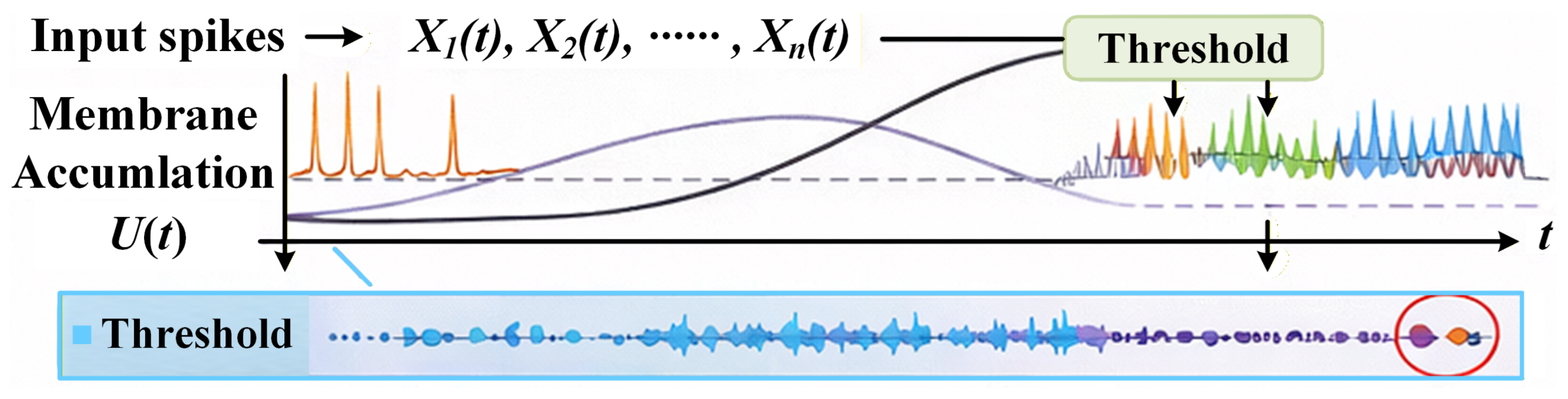
A commonly used neuron model is the leaky integrate-and-fire neuron, as shown in
Figure 2. In discrete time, the membrane potential update can be written as
where
is the membrane potential at time step
t,
is the leakage coefficient,
is the synaptic weight matrix,
is the bias term,
is the firing threshold, and
is the spike output at the previous time step.
The spike output is generated by a threshold function:
where
is the spike output at time step
t and
is the Heaviside step function.
where
a is the input variable of the threshold function.
After firing, the membrane potential is reset. A soft-reset form can be expressed as
where the membrane potential is reset after spike firing.
For a deep spiking layer
l, the dynamics can be further written as
where
denotes the membrane potential of the
l-th spiking layer,
is the leakage factor,
is the synaptic weight matrix, and
is the firing threshold of the
l-th layer.
where
is the spike output of the
l-th spiking layer and
is the total number of spiking layers.
For convolutional spiking networks, the matrix multiplication can be replaced by convolution:
where ∗ denotes the convolution operation and
is the convolution kernel of the
l-th layer.
Since the spike generation function is non-differentiable, direct backpropagation is difficult. Therefore, surrogate gradients are often used during training. Let
where
is a surrogate gradient function used to approximate the derivative of the non-differentiable spike function. A common choice is the rectangular surrogate function:
where
controls the width of the surrogate interval.
To obtain a static output from temporal spikes, the firing rate over all time steps can be used:
where
denotes the firing-rate representation obtained by averaging the spike outputs over all time steps. This formulation enables the network to model temporal dynamics while producing stable decision variables for compound fault detection.
2.3. Attention and Residual Learning in Deep Spiking Networks
Although spiking neural networks are suitable for temporal modeling, deep spiking architectures still face two problems. The first is response redundancy. Intermediate spiking features often contain both useful fault-related spikes and irrelevant responses. The second is information attenuation. As the network becomes deeper, weak impulsive information from shallow layers may gradually disappear.
To improve response selection, an attention mechanism can be introduced. Suppose that the spiking feature of a certain layer is denoted by
where
denotes the intermediate spiking feature tensor,
C is the number of channels,
T is the number of time steps, and
N is the spatial or feature dimension. Then a temporal attention descriptor can be obtained by channel aggregation:
where
is the temporal descriptor obtained by aggregating the feature tensor along the channel and spatial dimensions.
After linear transformation and normalization, the temporal attention weights are written as
where
denotes the temporal attention weights, and
and
are learnable parameters.
Similarly, the channel descriptor can be obtained by temporal–spatial aggregation:
where
is the channel descriptor obtained by aggregating the feature tensor along the temporal and spatial dimensions. The channel attention weights are
where
denotes the channel attention weights, and
and
are learnable parameters.
Then the refined feature can be written as
where
is the refined feature after temporal and channel reweighting.
This process allows the network to emphasize fault-sensitive channels and critical temporal responses at the same time.
However, attention alone cannot solve the problem of deep information attenuation. To preserve useful shallow features, residual learning is commonly adopted. For a standard residual block, the output can be written as
where
and
are the input and output features of the
l-th block, and
denotes the nonlinear transformation parameterized by
.
In a spiking framework, the residual transmission [
41] can be further controlled by a gating function. Let the gate coefficient be
where
is the gating coefficient and
is a learnable mapping function. Then the gated residual propagation can be written as
where ⊙ denotes element-wise multiplication. This equation means that the residual information is selectively transmitted under the control of the gate coefficient.
This method has two advantages. First, the residual path preserves shallow spiking information. Second, the gating mechanism can adaptively control the degree of information transmission. This is particularly useful for compound fault detection because weaker fault-related spiking responses can be more effectively preserved in deeper networks.
Based on the above analysis, combining attention mechanisms and residual learning within the spiking framework is a reasonable solution. The attention mechanism can improve the selection of key responses, while the residual gating mechanism can enhance information preservation. These two ideas provide the theoretical foundation for the method proposed in this paper.
3. Proposed Method
3.1. Overall Framework
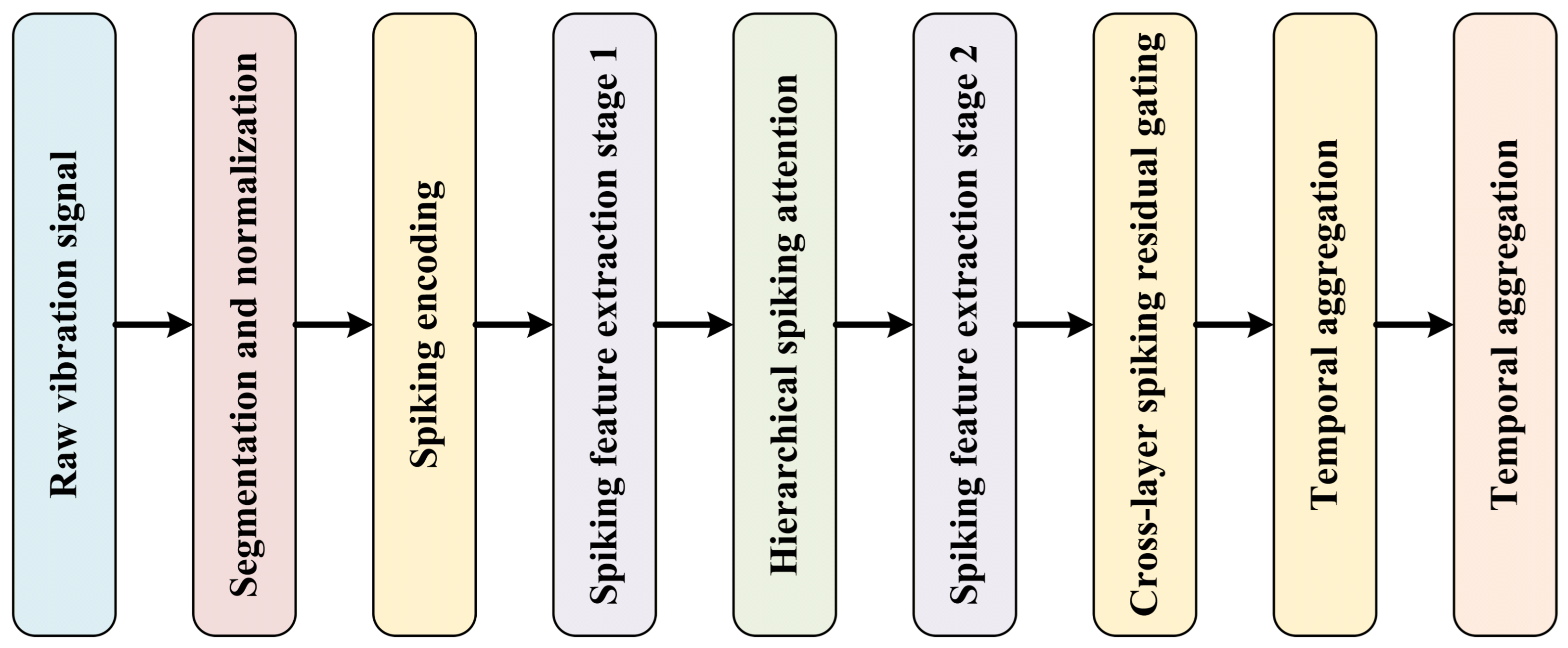
The overall structure of the proposed spiking attention residual network (SARN) is shown in
Figure 3. The network takes the raw time-domain vibration signal as input and performs compound fault detection in an end-to-end manner. The whole framework consists of four parts: signal segmentation and spiking encoding, hierarchical spiking feature extraction, spiking attention residual learning, and multi-label prediction.
Given an input vibration sample
, the signal is first divided into fixed-length segments and then converted into a spiking sequence. The encoded spiking input is written as
where
T is the number of spiking time steps, and
denotes the input spike tensor at time step
t.
The encoded sequence is then fed into several stacked spiking convolution blocks. These blocks extract hierarchical spiking features from shallow impulsive details to deep semantic representations. To improve the selection of fault-sensitive responses, a hierarchical spiking attention module is embedded into the feature learning process. At the same time, a cross-layer spiking residual gating mechanism is introduced to preserve useful shallow information during deep propagation.
After feature extraction, the final spiking representation is aggregated over time and passed to the multi-label output layer. The prediction vector is given by
where
C is the number of fault labels, and
denotes the predicted probability of the
c-th label.
The goal of the proposed method is to improve compound fault detection from two aspects. The first is response selection. The second is information preservation. The attention module helps the network focus on important spiking responses, while the residual gating mechanism stabilizes the propagation of weak fault information across layers.
3.2. Signal Segmentation and Spiking Encoding
The raw vibration signal is first normalized before it is fed into the network. For an input segment
, min-max normalization is used:
where
is the normalized signal value,
and
are the minimum and maximum values in the input segment, and
is a small constant used to avoid numerical instability.
After normalization, the signal is converted into a spiking sequence. In this work, temporal rate coding is adopted because of its simple form and stable implementation. The probability of spike generation at time step
t is defined as
where
denotes the spike generation probability of the
i-th signal point at time step
t. The input spike is generated by Bernoulli sampling:
where
is the generated spike at time step
t, and
is a random number uniformly sampled from
.
Thus, each signal segment is mapped to a spiking sequence over
T time steps:
where
denotes the spiking input matrix, whose rows correspond to different time steps and whose columns correspond to different signal positions.
This representation preserves the temporal structure of the original signal and transforms continuous vibration amplitudes into discrete spiking events. It also allows the following spiking network to process the signal in a temporal manner.
3.3. Hierarchical Spiking Feature Extraction
After spiking encoding, the input sequence is sent into a deep spiking feature extractor. The extractor is composed of several spiking convolution blocks. Each block contains a convolutional transformation, a spiking neuron layer, and a feature propagation path.
For the
l-th spiking convolution block, the membrane potential update is written as
where
is the membrane potential of the
l-th spiking layer at time step
t,
is the leakage factor,
is the convolution kernel,
is the input spike feature from the previous layer,
is the bias term, and
is the firing threshold.
The spike output of this layer is generated as
where
denotes the spike output of the
l-th layer at time step
t, and
is the Heaviside step function.
To better describe the temporal dynamics of compound fault signals, the hierarchical feature extraction process is performed across both space and time. Let the spiking feature of the
l-th layer be denoted as
where
denotes the temporal spiking feature sequence produced by the
l-th layer.
Then the deep extractor learns a mapping
where
denotes the spiking transformation of the
l-th block, and
is the parameter set of that block.
Through multiple spiking convolution blocks, the network gradually transforms low-level impulsive responses into high-level discriminative representations. However, in deep spiking networks, weak fault-related information may fade during this process. To address this issue, the proposed method introduces a hierarchical spiking attention module and a cross-layer spiking residual gating mechanism.
3.4. Hierarchical Spiking Attention Module
In compound fault signals, not all spiking responses are equally useful. Some responses are closely related to fault spikings, while others come from noise, background vibration, or irrelevant interference. Therefore, the network should assign larger weights to informative responses and smaller weights to redundant ones.
To achieve this, a hierarchical spiking attention module is designed. It consists of temporal attention and channel attention. The module is inserted after a spiking convolution block and acts on multi-level spiking features.
Let the input feature tensor of the attention module be
where
C is the number of channels,
T is the number of time steps, and
N is the feature length.
3.4.1. Temporal Attention
Temporal attention is used to identify important spiking responses over time. A temporal descriptor is first obtained by averaging the feature tensor over the channel and feature dimensions:
where
denotes the temporal descriptor at the
t-th time step.
The temporal descriptor vector is written as
where
is the temporal descriptor vector composed of all time-step descriptors.
Then the temporal attention weights are generated by
where
denotes the temporal attention weight vector, and
and
are learnable parameters.
The temporally refined feature is given by
where
denotes the feature refined by temporal attention, and
is the temporal attention weight at time step
t.
This operation helps the network focus on key time steps that contain fault-sensitive impulsive responses.
3.4.2. Channel Attention
Different channels usually capture different aspects of the fault pattern. Some channels are more sensitive to compound fault characteristics than others. Therefore, channel attention is used to adaptively recalibrate channel importance.
The channel descriptor is obtained by averaging along the temporal and feature dimensions:
where
denotes the descriptor of the
c-th channel.
The channel descriptor vector is
where
is the channel descriptor vector formed by all channel descriptors.
Then the channel attention weights are computed as
where
denotes the channel attention weight vector, and
and
are trainable parameters.
The channel-refined feature is written as
where
denotes the feature refined by channel attention, and
is the weight assigned to the
c-th channel.
3.4.3. Joint Spiking Attention Refinement
To combine temporal attention and channel attention, the two weight maps are jointly applied to the input feature:
where
denotes the jointly refined feature after temporal and channel reweighting. For stable training, a residual refinement form is used:
where
is the final output feature of the hierarchical spiking attention module. This formulation allows the original feature and the refined feature to be preserved together. It also reduces the risk of over-suppressing useful spiking responses.
The hierarchical spiking attention module is applied to several stages of the network. In this way, the model can emphasize important responses at different feature levels, from shallow impulsive details to deep semantic patterns.
3.5. Cross-Layer Spiking Residual Gating Mechanism
Although the attention module improves response selection, deep spiking networks still suffer from information attenuation. In particular, shallow layers often contain local impulsive details, but these details may gradually vanish in deep layers. This is harmful for compound fault detection, especially when weak fault features are present.
To solve this problem, a cross-layer spiking residual gating mechanism is introduced. The basic idea is to preserve shallow information and adaptively transmit it to deeper layers.
Let
be the input feature of the
l-th block. Its transformed feature is
where
denotes the transformed feature of the
l-th block,
is the nonlinear mapping function, and
is the parameter set of the current block.
A gate coefficient is then generated from the current feature:
where
is the gate coefficient, and
denotes a learnable gating function.
The output of the gated residual block is written as
where
is the output feature of the next block, and ⊙ denotes element-wise multiplication.
This equation means that the residual information is not directly added in a fixed way. Instead, it is controlled by the gate coefficient. If a shallow response is useful, the gate tends to assign a larger value and preserve it. If the response is less useful, the gate suppresses its propagation.
To further improve cross-layer fusion, an inter-layer residual aggregation form can also be written as
where
denotes the learnable transmission coefficient from the
k-th layer to the
l-th layer.
The proposed residual gating mechanism has two advantages. First, it improves the stability of deep feature propagation. Second, it preserves weak impulsive information from shallow layers. Both are important for recognizing compound fault patterns.
3.6. Multi-Label Optimization Objective
After the last spiking feature extraction stage, the output spikes are aggregated over time by average firing rate:
where
is the aggregated firing-rate feature, and
denotes the index of the last spiking layer.
The aggregated feature
is then fed into the output layer:
where
denotes the output logits, and
and
are the weight matrix and bias vector of the output layer.
The prediction of each fault label is obtained through the sigmoid function:
where
is the predicted multi-label probability vector.
For multi-label compound fault detection, the binary cross-entropy loss is used as the main optimization objective:
where
denotes the classification loss for multi-label learning.
To stabilize attention learning, an
regularization term can be added:
where
is the regularization loss,
p denotes a trainable parameter, and
is the set of all trainable parameters.
Thus, the final loss function is
where
is the regularization coefficient used to balance the classification loss and the regularization term.
During inference, the binary decision of each label is determined by
where
is the final binary prediction of the
c-th label, and
is the decision threshold.
This strategy allows the model to identify multiple fault attributes in one sample. It is therefore more suitable for compound fault detection than ordinary single-label classification.
3.7. Discussion of the Proposed Method
The SARN model proposed in this paper addresses two key issues in compound fault detection. The first is how to highlight fault-sensitive spiking responses. The second is how to preserve weak but useful information in deep spiking architectures.
A hierarchical spiking attention module solves the first problem. It emphasizes important temporal responses and information-rich channels. A cross-layer spiking residual gating mechanism solves the second problem. It improves the propagation of shallow spiking details and reduces information loss in deeper layers. Finally, a multi-label output layer makes the framework more consistent with the nature of compound fault detection.
Therefore, the proposed method integrates spiking feature learning, attention-based response selection, residual-based information preservation, and multi-label modeling into a unified framework. This lays the foundation for the experiments and analyses in subsequent chapters.
4. Experimental Verification
4.1. Experimental Dataset
The experimental data is organized around a compound fault detection task with multi-label output. As shown in
Table 1, each sample of this dataset is associated with three sub-labels to simultaneously describe different fault attributes. This setup matches the output format of the proposed method, avoiding representing each compound fault state as a completely independent category. A total of 11 bearing states were considered in the experiments. These states include a normal state, several single fault states, and several compound fault states composed of combinations of different single faults.
Detailed definitions of these states are summarized in
Table 2.
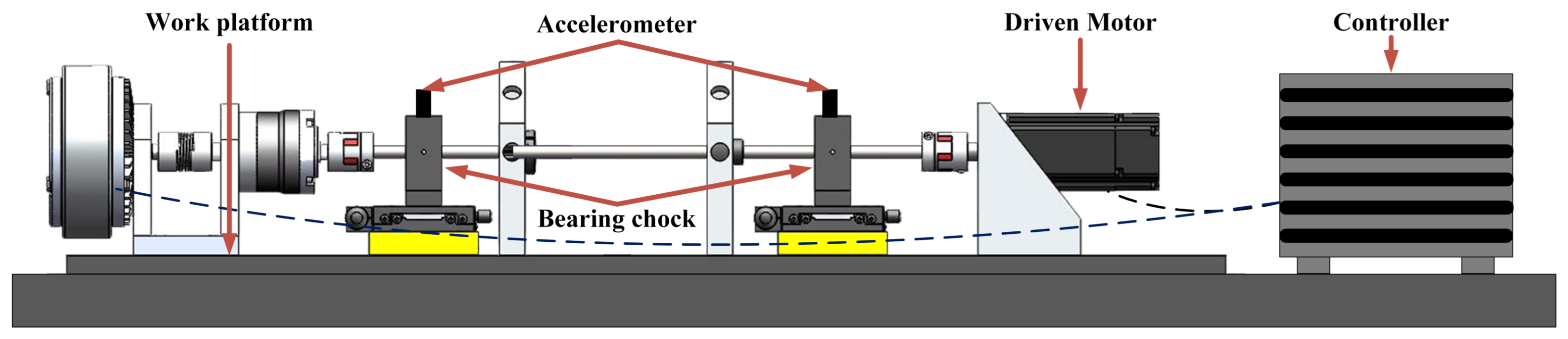
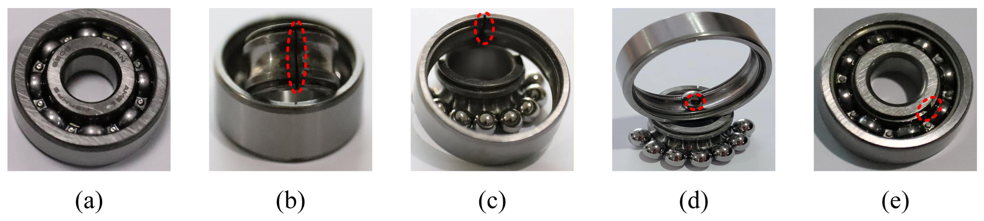
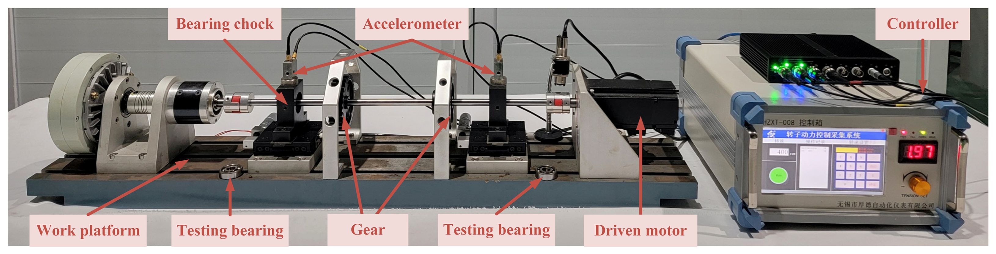
Figure 4 shows some representative bearings. From a task perspective, this dataset is challenging because it contains both simple and coupled fault modes, and the boundaries between some states are not obvious. The data was collected on a laboratory bearing test bench. The overall structure of the platform is shown in
Figure 5, and a simplified layout is shown in
Figure 6. The main components include a drive motor, bearing housing, a faulty bearing mounted on the drive end, and an accelerometer mounted near the bearing. During data acquisition, the sampling frequency was set to 49,152 Hz, and the rotational speed was fixed at 1500 rpm. Specifically, the bearing parameters are: manufacturer NSK (Tokyo, Japan), bearing specification 6200, pitch diameter 20 mm, roller number 8, roller diameter 5 mm, and contact angle 0°.
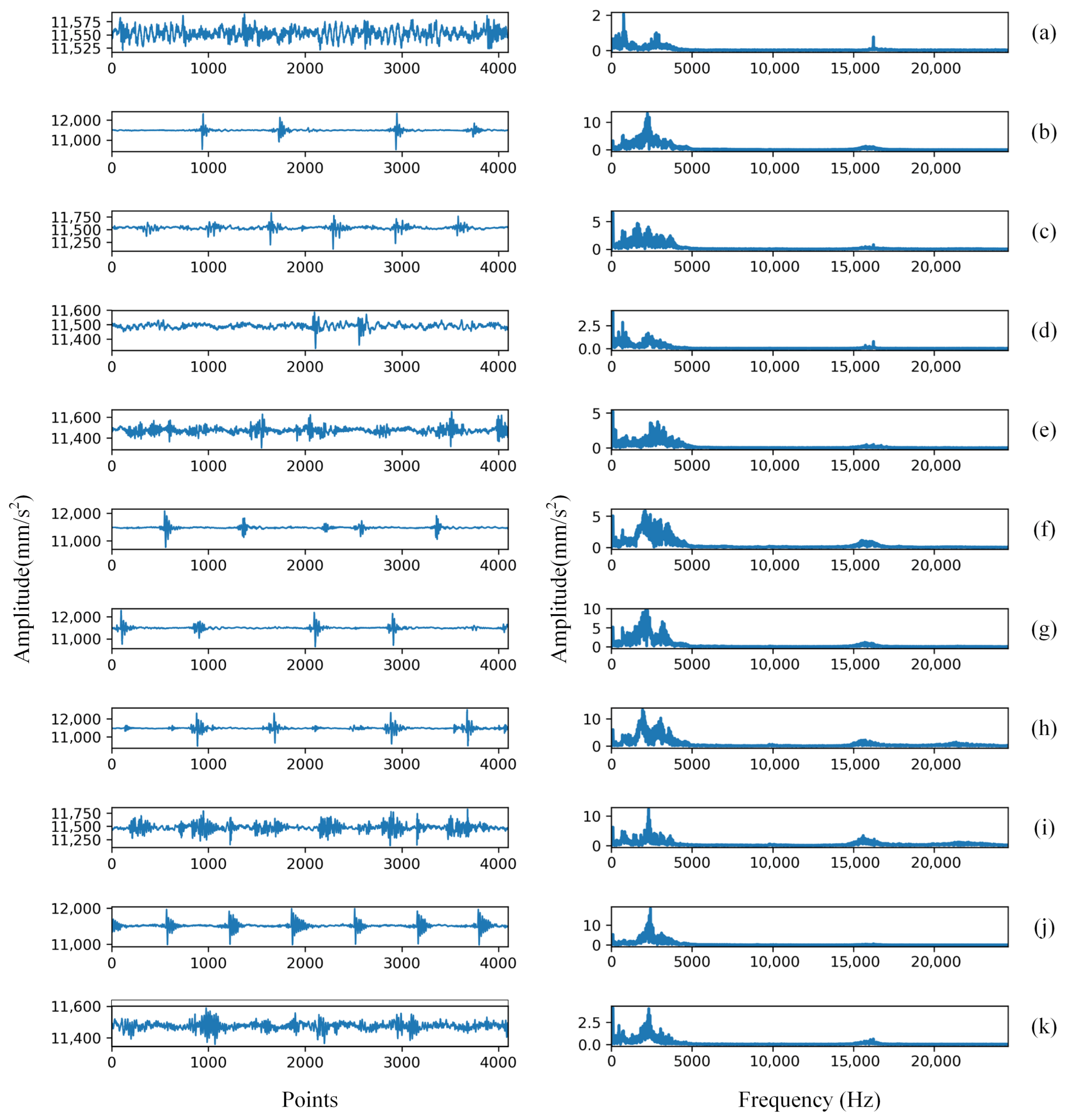
Figure 7 shows the time-domain signals under 11 states. Some states exhibit significant pulse differences, but some single-fault and compound-fault cases still show significant overlap in the waveform domain. This indicates that it is difficult to separate the dataset based solely on the raw signals. This also explains why compound fault detection requires models with stronger representational capabilities. Regarding sample construction, the raw vibration signal was segmented into fixed-length samples. Each sample contains 4096 data points. To improve the diversity of the training set, data augmentation was performed after segmentation. Therefore, the number of normal samples and fault samples for each state was set to 200 and 50, respectively. This sample construction strategy ensures consistent data format across all states and provides a unified basis for model comparison.
4.2. Experimental Settings
This experiment aims to answer a key question: does the proposed SARN method provide more efficient feature learning and more suitable output modeling for compound fault detection than existing methods. To answer this question, we selected several comparative models from two categories. The first category includes traditional multi-label classifiers, including BR, CC, LP, ML-KNN, and Rank-SVM. These methods are used to demonstrate the ability of shallow multi-label learning on compound fault data. The second category includes deep learning baseline models to compare the hierarchical representation capabilities of different methods on raw vibration signals, including ML-CNN (Multi-label CNN), ATT-ML-CNN (ML-CNN with attention mechanism), and the proposed SARN. Specifically, ML-CNN is a conventional convolutional neural network adapted for multi-label fault classification on raw vibration data. ATT-ML-CNN further introduces an attention mechanism to enhance the extraction of informative local patterns and improve label-related feature aggregation. SARN is the proposed method of this study, which integrates pulse-based hierarchical representation learning and residual attention modeling to better characterize the coupling relationships and structural dependencies in compound fault signals. The comparative methods are listed in
Table 3.
The encoded sequence is processed by a pulse backbone network, a hierarchical pulse attention module, and a cross-layer pulse residual gating mechanism, and finally mapped to the multi-label output. To ensure fair comparison, all methods are evaluated on the same dataset split. The same sample construction strategy and label settings are used throughout the experiment. For the proposed SARN model, the optimization objective follows the multi-label loss defined in
Section 3.6. Thus, the comparison focuses on differences in feature extraction and model design, rather than inconsistencies in output settings.
All models were implemented in the same development environment. The deep models were built on the PyTorch platform, while the spiking part of the proposed method was implemented using a dedicated spiking neural network package. The main hyperparameters of SARN include the number of spiking timesteps, trigger threshold, leakage coefficient, learning rate, batch size, and regularization coefficient. These parameters were determined through initial tuning and remained constant in all formal experiments.
4.3. Results and Discussion
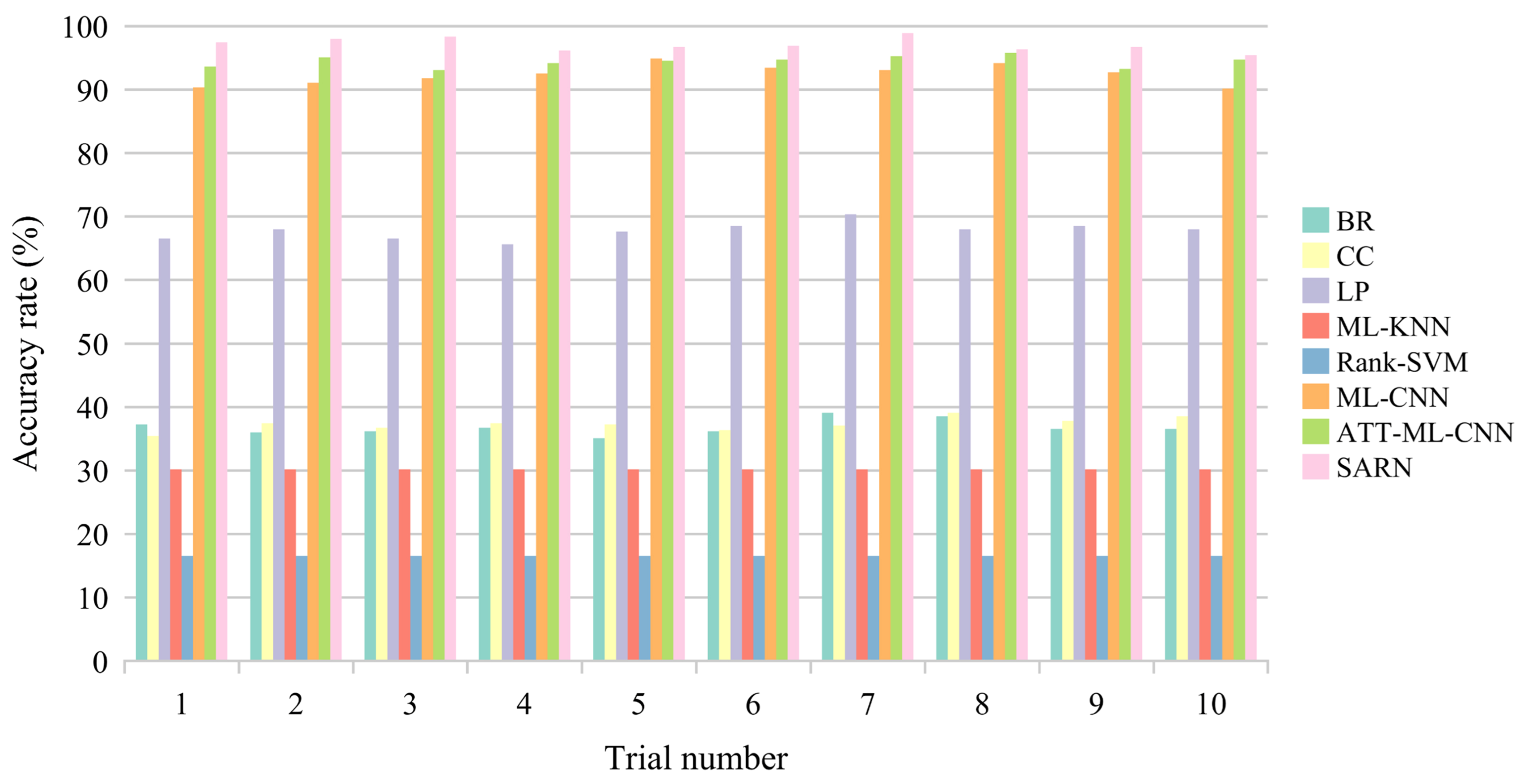
Experimental results are shown in
Figure 8, and statistical comparison results are summarized in
Table 4. The proposed SARN achieves the best overall performance among all compared methods. Its average accuracy and F1 score are both higher than traditional multi-label methods and deep learning baseline methods. This result verifies the effectiveness of the proposed framework in compound fault detection.
The five traditional multi-label methods have relatively low performance. This indicates that shallow models are insufficient for compound fault identification. Although they can model multiple labels, they cannot effectively learn discriminative features from strongly coupled vibration signals.
The deep learning baseline methods outperform traditional methods, confirming the value of hierarchical feature learning. However, their results are still inferior to SARN. This difference is consistent with the design in
Section 3. The hierarchical spiking attention module improves the selection of fault-sensitive responses by emphasizing important temporal responses and information-rich channels. Therefore, redundant responses are suppressed, and useful compound fault features are enhanced.
The cross-layer spiking residual gating mechanism also contributes to performance improvement. In compound fault signals, weaker spiking components are easily masked by stronger responses. If shallow fault details are not preserved during deep propagation, the final representation’s discriminative power will decrease. Residual gating paths mitigate this problem by selectively preserving useful shallow information. This explains why SARN not only has higher accuracy but also better stability in repeated runs.
The multi-label output strategy further improves the consistency between the model output and the task itself. Since a compound fault sample may contain multiple fault attributes, multi-label formulations are more suitable than ordinary single-label classification. Therefore, SARN’s performance improvement comes not only from better feature extraction but also from a more suitable output formulation.
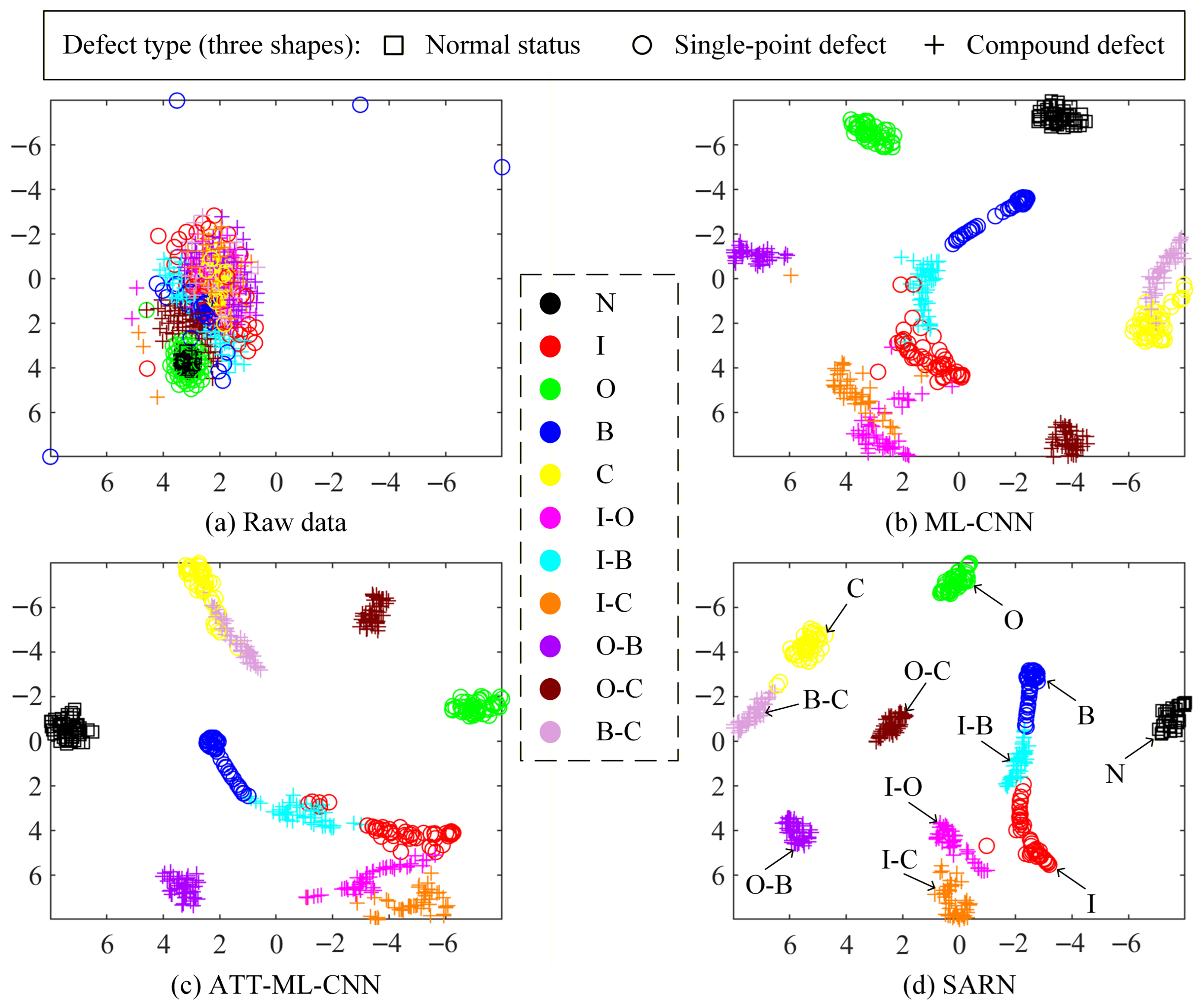
To further compare feature extraction capabilities, we visualize the learned features using t-SNE, as shown in
Figure 9.
Figure 9a shows the original data distribution. Samples from different states overlap significantly, indicating poor separability in the original space.
Figure 9b,c show the features learned by the baseline deep model. Their clustering performance is improved, but overlap still exists between several compound fault states.
Figure 9d shows the features learned by SARN. The clustering is more compact, and the boundaries between different states are clearer.
This visualization result is consistent with the quantitative results in
Table 4. The clearer distribution of SARN features indicates that the proposed network extracts more discriminative representations. Specifically, the attention module improves the selection of key responses, and the residual gating mechanism improves the preservation of depth information. Combined with a multi-label output strategy, the proposed method constructs a coherent framework for compound fault detection. Overall, the results show that SARN has better recognition performance, stronger feature separability, and more stable detection behavior compared to the contrasting methods.
5. Conclusions
In this paper, a spiking attention residual network (SARN) was proposed for compound fault detection. The proposed method directly uses raw time-domain vibration signals as input and builds an end-to-end spiking neural network framework. To improve the representation of coupled fault patterns, a hierarchical spiking attention module was introduced to enhance critical temporal responses and fault-sensitive channels. Meanwhile, a cross-layer spiking residual gating mechanism was designed to preserve useful shallow impulsive information during deep propagation. In addition, a multi-label detection strategy was adopted to jointly identify multiple fault attributes, which is more consistent with the nature of compound faults. Experimental results show that the proposed method achieves better accuracy, F1-score, feature separability, and detection stability than the compared methods. These results demonstrate that improving response selection and information preservation in deep spiking networks is effective for compound fault detection.
Although the proposed method obtained promising results, several issues still deserve further study. First, the current verification was conducted on a laboratory dataset, and broader validation on more complex industrial datasets is still needed. Second, the present model mainly focuses on supervised compound fault detection, while transferability under varying machines, working conditions, and limited labeled samples remains to be explored. Third, the spiking encoding strategy and attention-residual interaction can be further optimized to improve efficiency and interpretability. In future work, we will extend the proposed framework to more practical industrial scenarios, investigate lightweight and transferable spiking architectures, and study more adaptive multi-label learning mechanisms for complex compound fault diagnosis tasks.




 and
and