Figure 1.
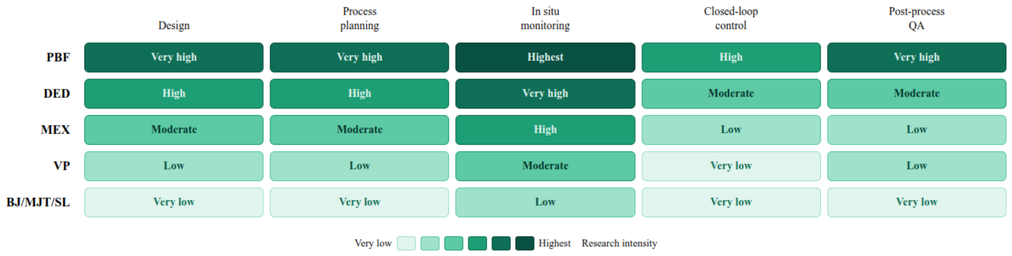
AI/ML integration across the AM life cycle. Heatmap of relative research maturity by process family and life cycle stage.
Figure 1.
AI/ML integration across the AM life cycle. Heatmap of relative research maturity by process family and life cycle stage.
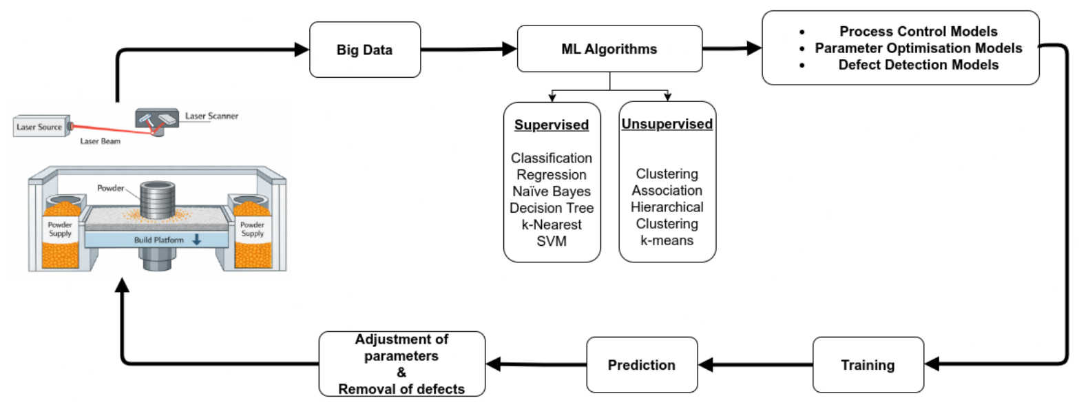
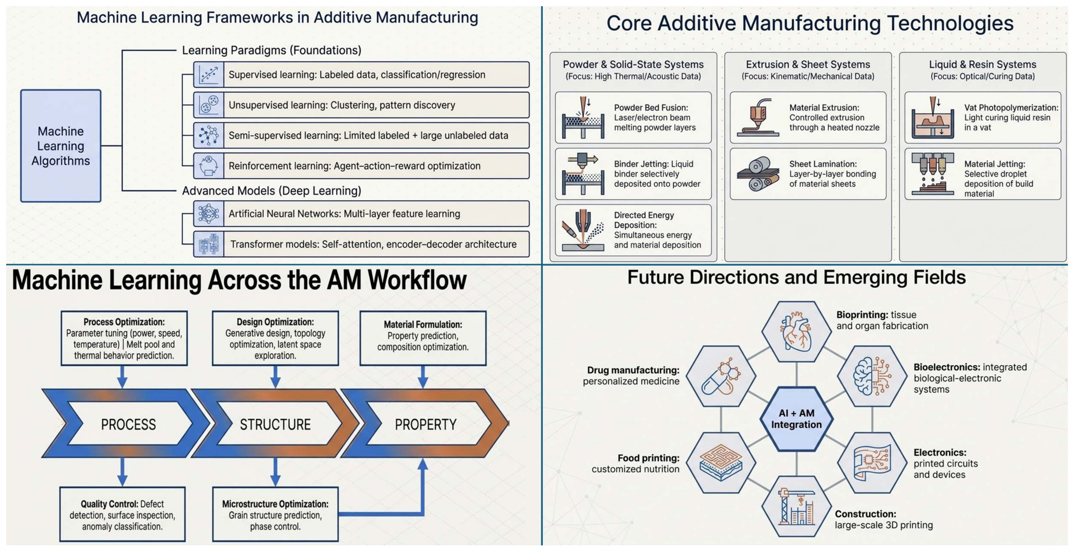
Figure 2.
Generalized framework for the integration of machine learning in additive manufacturing applications, showing the workflow from data acquisition through model deployment.
Figure 2.
Generalized framework for the integration of machine learning in additive manufacturing applications, showing the workflow from data acquisition through model deployment.
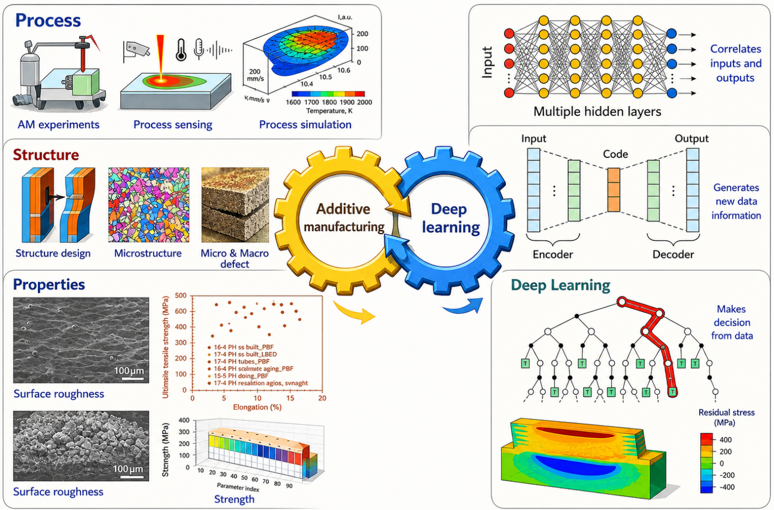
Figure 3.
Application areas of deep learning in additive manufacturing, spanning design optimization, process control, monitoring, and quality assurance.
Figure 3.
Application areas of deep learning in additive manufacturing, spanning design optimization, process control, monitoring, and quality assurance.
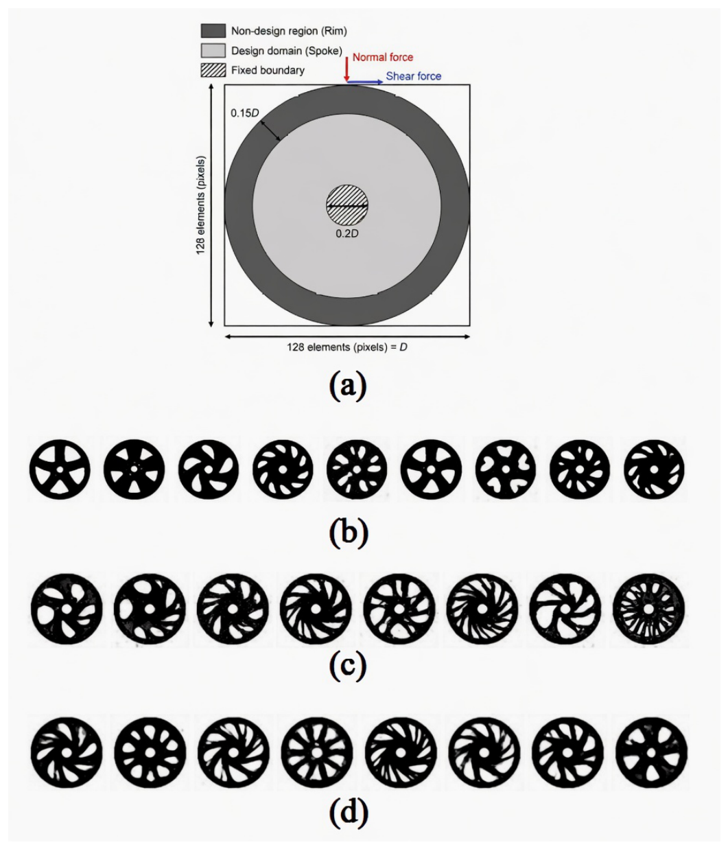
Figure 4.
(
a) Domain and boundary conditions of a 2D wheel design; (
b) generative adversarial network (GAN); (
c) deep convolutional GANs (DCGANs); (
d) variational autoencoder (VAE) architectures [
45].
Figure 4.
(
a) Domain and boundary conditions of a 2D wheel design; (
b) generative adversarial network (GAN); (
c) deep convolutional GANs (DCGANs); (
d) variational autoencoder (VAE) architectures [
45].
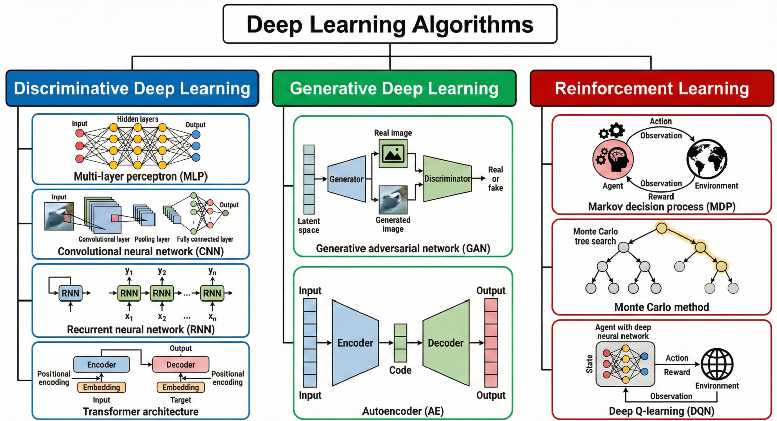
Figure 5.
Three types of deep learning algorithms: discriminative DL for classification/regression, generative DL for data synthesis, and reinforcement learning for decision-making.
Figure 5.
Three types of deep learning algorithms: discriminative DL for classification/regression, generative DL for data synthesis, and reinforcement learning for decision-making.
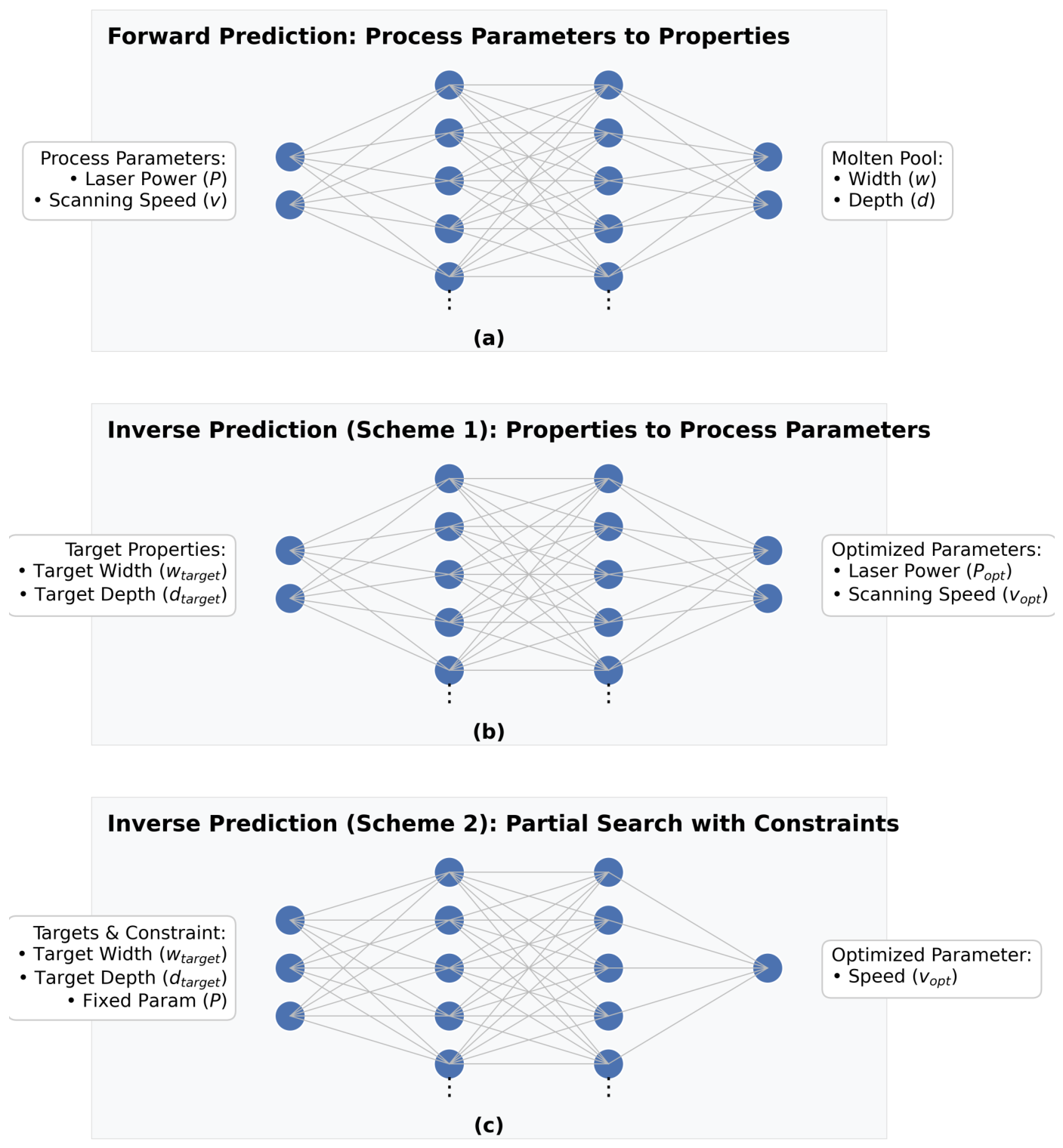
Figure 7.
Illustration of the bidirectional predictions: (a) forward prediction from process parameters to molten pool dimensions; (b) Scheme 1 of the inverse prediction, from molten pool dimensions to process parameters; (c) Scheme 2 of the inverse prediction, where the input has three variables (i.e., one process variable and two molten pool dimensions).
Figure 7.
Illustration of the bidirectional predictions: (a) forward prediction from process parameters to molten pool dimensions; (b) Scheme 1 of the inverse prediction, from molten pool dimensions to process parameters; (c) Scheme 2 of the inverse prediction, where the input has three variables (i.e., one process variable and two molten pool dimensions).
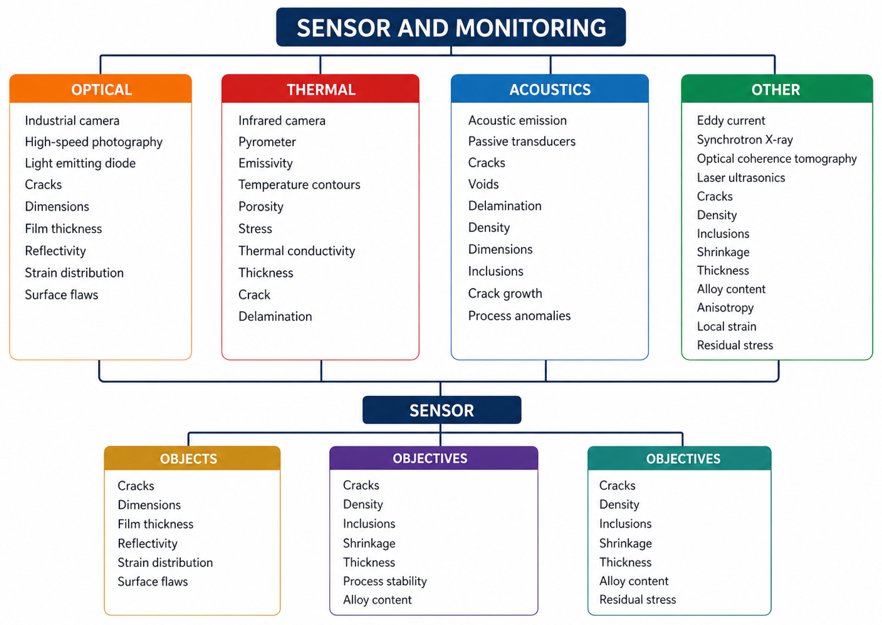
Figure 8.
Sensors, signals, and objectives commonly used for monitoring in additive manufacturing, including optical cameras, pyrometers, acoustic sensors, and spectroscopic methods.
Figure 8.
Sensors, signals, and objectives commonly used for monitoring in additive manufacturing, including optical cameras, pyrometers, acoustic sensors, and spectroscopic methods.
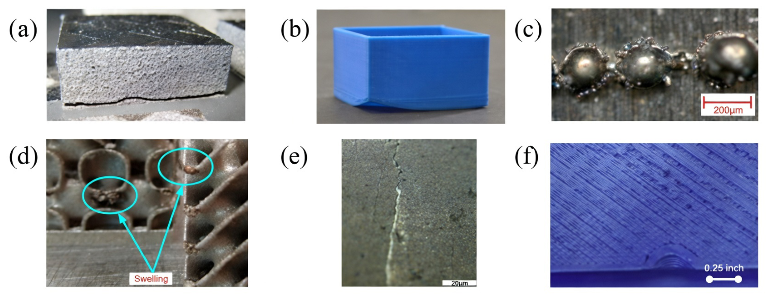
Figure 9.
Typical examples of defects in additive manufacturing showing: (
a) macro-cracks, (
b) warping, (
c) balling, (
d) swelling, (
e) micro-cracks, and (
f) an under-filled part [
90]. Dimensions in subfigures (
c,
e) are in micrometers (μm), whereas subfigure (
f) is in inches (in).
Figure 9.
Typical examples of defects in additive manufacturing showing: (
a) macro-cracks, (
b) warping, (
c) balling, (
d) swelling, (
e) micro-cracks, and (
f) an under-filled part [
90]. Dimensions in subfigures (
c,
e) are in micrometers (μm), whereas subfigure (
f) is in inches (in).
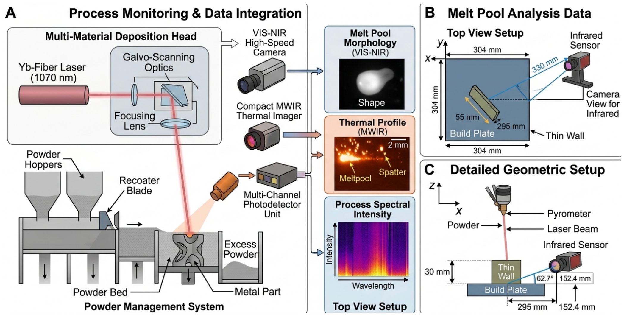
Figure 10.
Sensor configurations for melt pool monitoring in laser-based additive manufacturing: (A) LPBF/SLM process with coaxial and off-axis sensing; (B) top-view measurement geometry; (C) side-view sensor configuration.
Figure 10.
Sensor configurations for melt pool monitoring in laser-based additive manufacturing: (A) LPBF/SLM process with coaxial and off-axis sensing; (B) top-view measurement geometry; (C) side-view sensor configuration.
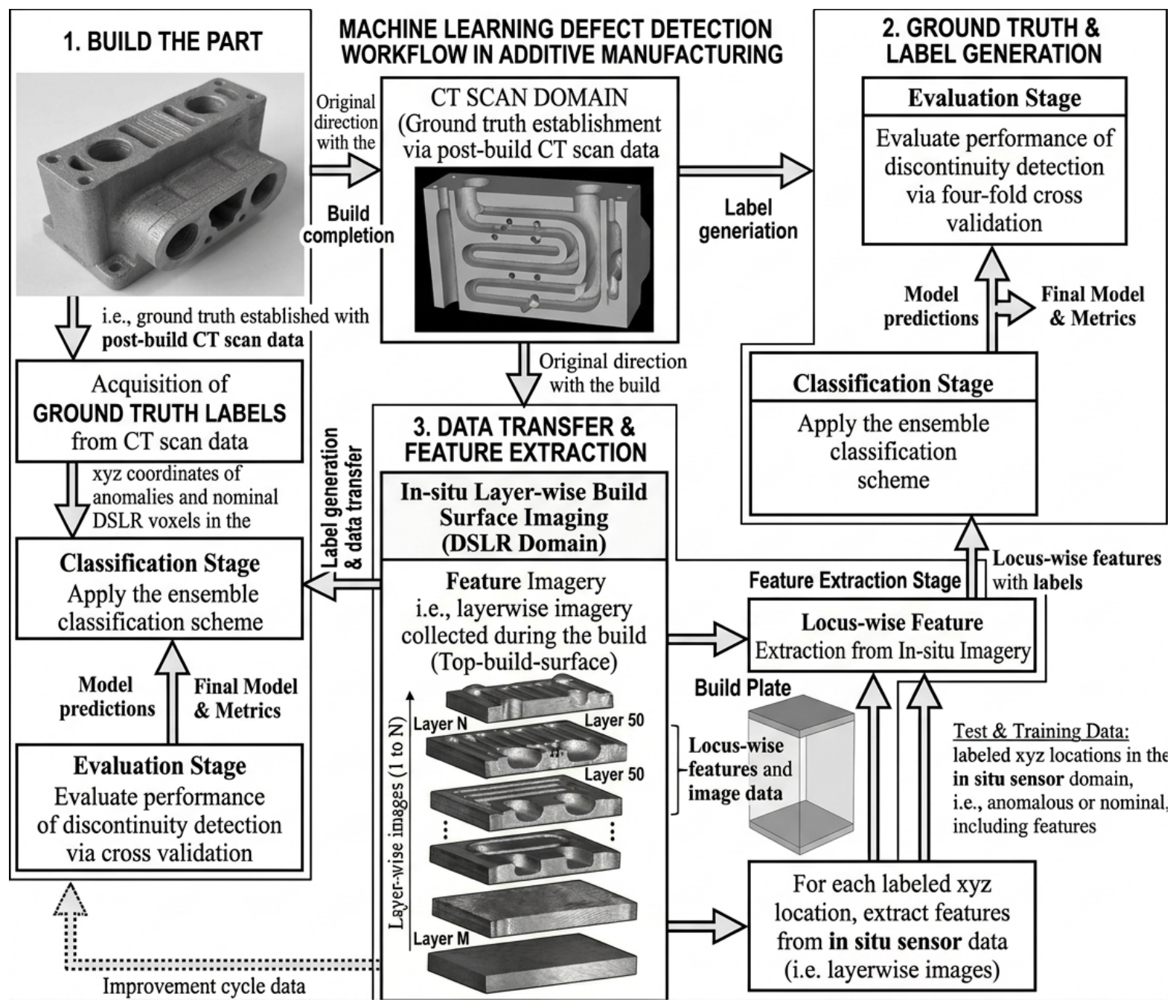
Figure 11.
Flowchart of ML techniques for defect detection in SLM processing using in situ layer-wise top build surface imaging, showing preprocessing, feature extraction, and classification stages.
Figure 11.
Flowchart of ML techniques for defect detection in SLM processing using in situ layer-wise top build surface imaging, showing preprocessing, feature extraction, and classification stages.
Figure 12.
Distribution of ML algorithms and approaches used in DED additive manufacturing research, showing the prevalence of neural network methods and the growth of physics-informed approaches.
Figure 12.
Distribution of ML algorithms and approaches used in DED additive manufacturing research, showing the prevalence of neural network methods and the growth of physics-informed approaches.
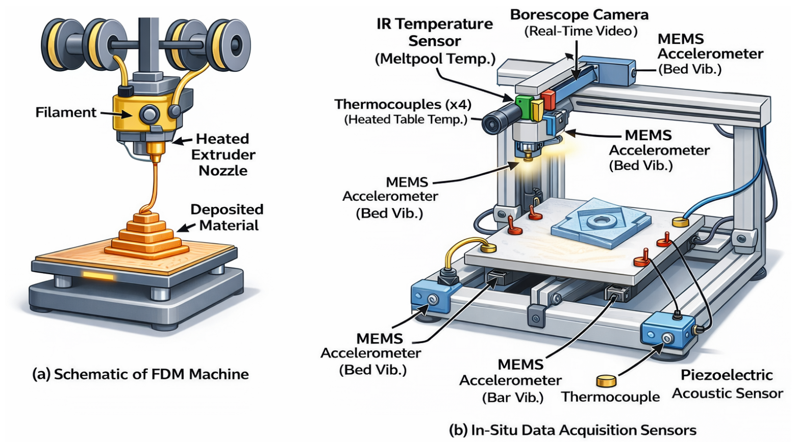
Figure 13.
(a) Schematic of FDM machine showing key components, and (b) multiple sensors implemented for in situ data acquisition including cameras, thermocouples, accelerometers, and acoustic sensors.
Figure 13.
(a) Schematic of FDM machine showing key components, and (b) multiple sensors implemented for in situ data acquisition including cameras, thermocouples, accelerometers, and acoustic sensors.
Figure 14.
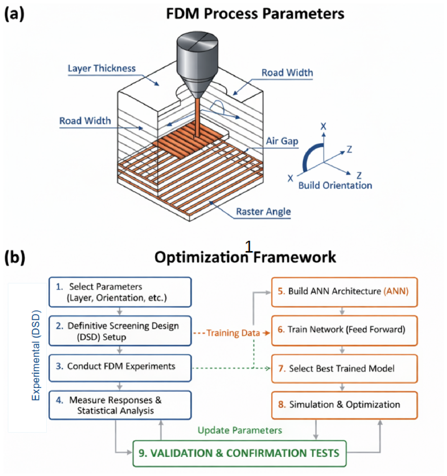
Schematic of FDM using definitive screening design (DSD) and deep learning feedforward ANN: (a) FDM process variables including layer thickness, raster gap, build orientation, road width, and number of contours; (b) neural network architecture for process parameter optimization.
Figure 14.
Schematic of FDM using definitive screening design (DSD) and deep learning feedforward ANN: (a) FDM process variables including layer thickness, raster gap, build orientation, road width, and number of contours; (b) neural network architecture for process parameter optimization.
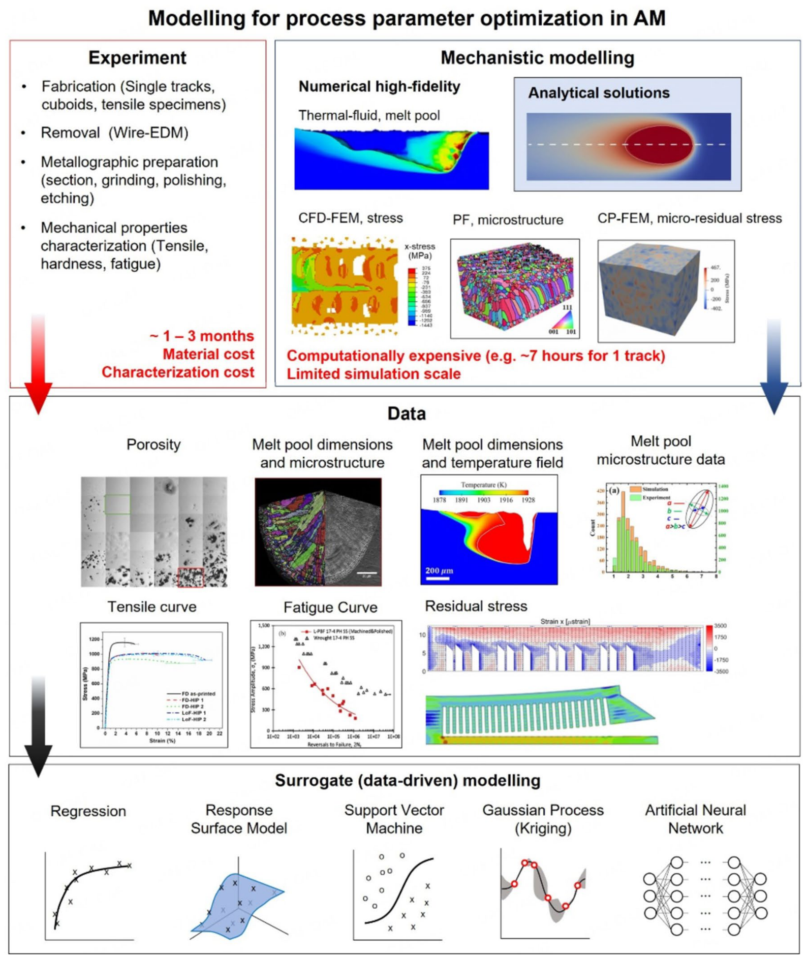
Figure 15.
Framework for ML-based process parameter optimization in AM, illustrating the iterative cycle of experimental data collection, model training, prediction, and optimization [
38].
Figure 15.
Framework for ML-based process parameter optimization in AM, illustrating the iterative cycle of experimental data collection, model training, prediction, and optimization [
38].
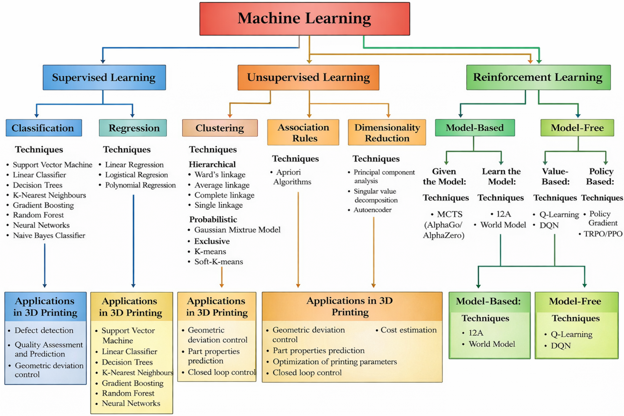
Figure 16.
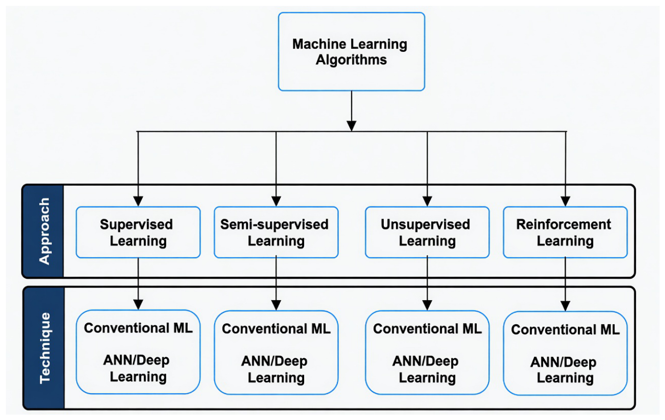
Taxonomy of ML types (supervised, unsupervised, reinforcement learning) and their applications to different areas of 3D printing, including design optimization, process control, and quality assurance.
Figure 16.
Taxonomy of ML types (supervised, unsupervised, reinforcement learning) and their applications to different areas of 3D printing, including design optimization, process control, and quality assurance.
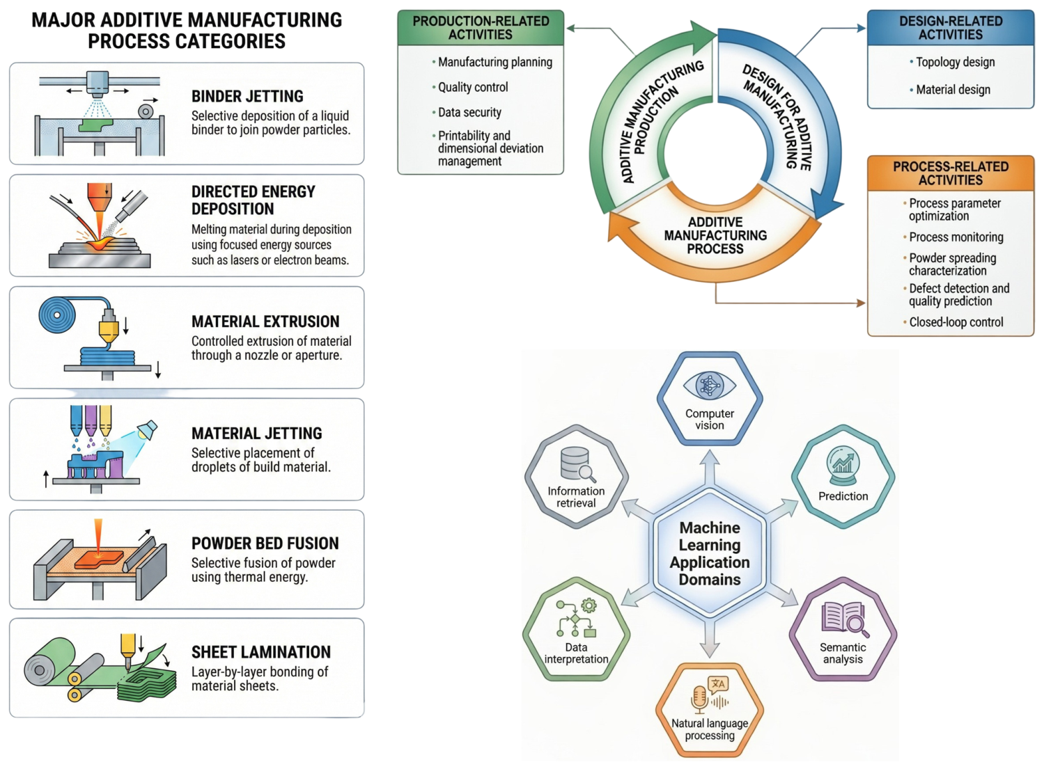
Figure 17.
Categorization of additive manufacturing processes and their corresponding machine learning application areas, illustrating the diversity of opportunities for AI/ML integration across process families. The arrows within the Additive Manufacturing Process cycle (top right) detail the iterative relationship between design, production, and process activities. Specifically, they show the flow from design-related activities (e.g., topology design) through additive manufacturing production, and into production-related activities (e.g., quality control), with feedback loops indicating iterative improvement and optimization. This schema explicitly separates design optimization pathways (e.g., topology/generative design) from process optimization pathways (e.g., parameter tuning, monitoring, and control).
Figure 17.
Categorization of additive manufacturing processes and their corresponding machine learning application areas, illustrating the diversity of opportunities for AI/ML integration across process families. The arrows within the Additive Manufacturing Process cycle (top right) detail the iterative relationship between design, production, and process activities. Specifically, they show the flow from design-related activities (e.g., topology design) through additive manufacturing production, and into production-related activities (e.g., quality control), with feedback loops indicating iterative improvement and optimization. This schema explicitly separates design optimization pathways (e.g., topology/generative design) from process optimization pathways (e.g., parameter tuning, monitoring, and control).
Figure 18.
Summary of machine learning integration across additive manufacturing processes, showing diverse optimization and application areas spanning design, process control, monitoring, and quality assurance.
Figure 18.
Summary of machine learning integration across additive manufacturing processes, showing diverse optimization and application areas spanning design, process control, monitoring, and quality assurance.
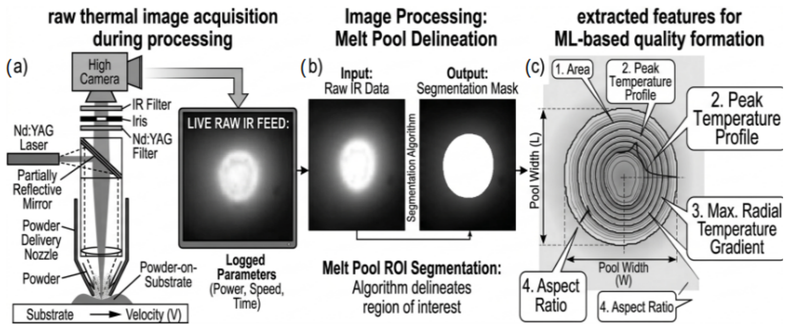
Figure 19.
Melt pool analysis using infrared thermal imaging: (a) raw thermal image acquisition during processing, (b) segmented melt pool region, and (c) extracted features for ML-based quality prediction. This workflow exemplifies the data processing pipeline required for intelligent monitoring systems.
Figure 19.
Melt pool analysis using infrared thermal imaging: (a) raw thermal image acquisition during processing, (b) segmented melt pool region, and (c) extracted features for ML-based quality prediction. This workflow exemplifies the data processing pipeline required for intelligent monitoring systems.
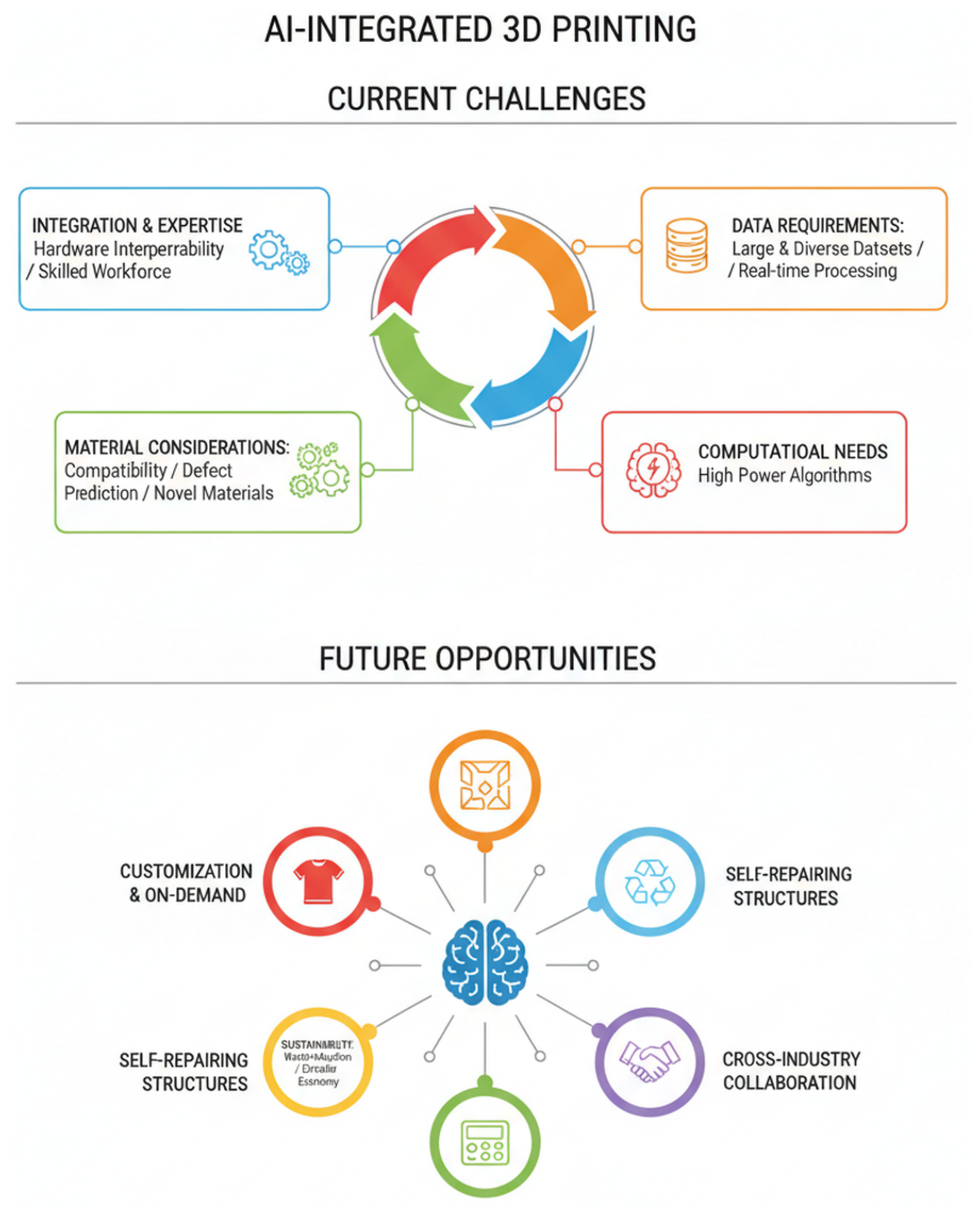
Figure 20.
Current challenges and future prospects of AI-integrated 3D printing, highlighting data requirements, computational needs, material considerations, and sustainability opportunities.
Figure 20.
Current challenges and future prospects of AI-integrated 3D printing, highlighting data requirements, computational needs, material considerations, and sustainability opportunities.
Figure 21.
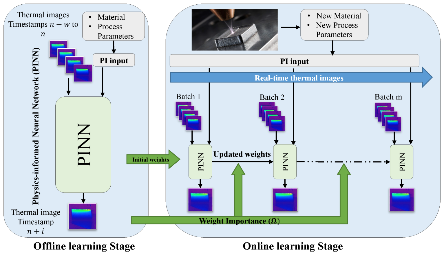
Overview of a two-stage Physics-informed neural networks (PINN) based framework for online 2D temperature field prediction in metal additive manufacturing. The model is guided by physics-informed inputs derived from process parameters and material properties, initially trained on pre-existing thermal datasets and subsequently updated using real-time thermal imaging [
144].
Figure 21.
Overview of a two-stage Physics-informed neural networks (PINN) based framework for online 2D temperature field prediction in metal additive manufacturing. The model is guided by physics-informed inputs derived from process parameters and material properties, initially trained on pre-existing thermal datasets and subsequently updated using real-time thermal imaging [
144].
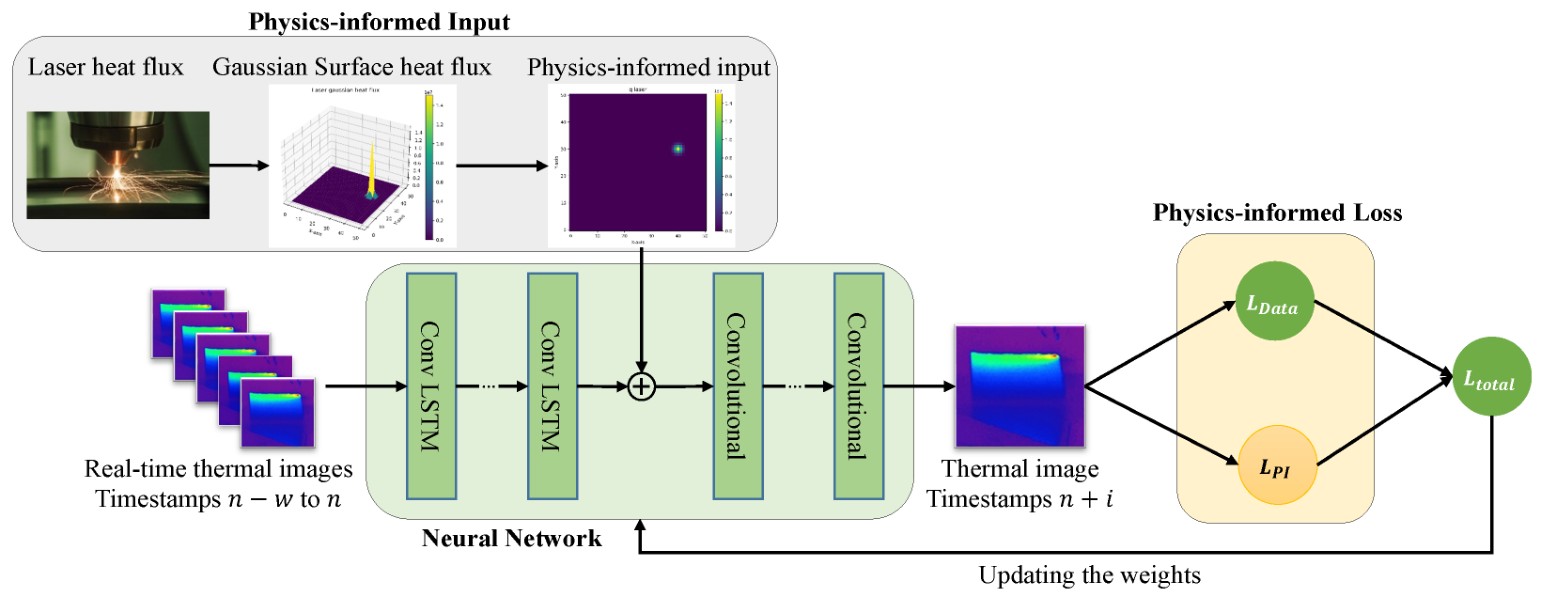
Figure 22.
Schematic of the proposed physics-informed neural network (PINN) framework, comprising the neural network, physics-informed input, and physics-informed loss used for thermal field prediction in metal additive manufacturing [
144].
Figure 22.
Schematic of the proposed physics-informed neural network (PINN) framework, comprising the neural network, physics-informed input, and physics-informed loss used for thermal field prediction in metal additive manufacturing [
144].
Table 1.
ISO/ASTM standards referenced in this review and their role in manuscript organization.
Table 1.
ISO/ASTM standards referenced in this review and their role in manuscript organization.
| Standard | Scope | Use in This Manuscript |
|---|
| ISO/ASTM 52900:2021; Additive manufacturing—General principles—Fundamentals and vocabulary [24] | Terminology and process-family definitions | Defines the seven AM process families used for section-level organization and terminology normalization. |
| Process-family taxonomy derived from ISO/ASTM 52900:2021 [24] | Classification framework | Supports cross-process comparison of AI/ML maturity, data modalities, and life cycle deployment status. |
| Journal formatting requirements | Tables, figures, references style | Guides formatting updates for captions, citations, and nomenclature presentation in the revised draft. |
Table 2.
Comparison of classical ML algorithms for AM applications.
Table 2.
Comparison of classical ML algorithms for AM applications.
| Algorithm | Data Requirements | Typical AM Applications | Advantages | Limitations |
|---|
| SVM | Small–medium datasets; works with features | Defect classification; process window identification | Effective in high dimensions; robust to overfitting | Sensitive to hyperparameters; limited scalability |
| Random Forest | Medium–large; handles missing data | Property prediction; feature importance analysis | Interpretable; handles nonlinearity; ensemble robustness | Memory intensive; slow for real-time |
| Gradient Boosting (XGBoost) | Medium–large; structured data | Process optimization; quality prediction | High accuracy; built-in regularization | Prone to overfitting; sensitive to noise |
| Gaussian Process | Small datasets preferred | Surrogate modeling; uncertainty quantification; active learning | Provides uncertainty; few hyperparameters | Scales poorly ; assumes smooth functions |
| k-NN | Any size; distance-based | Anomaly detection; similarity search | Simple; no training; adaptable | Slow at inference; sensitive to dimensionality |
| ANN (Shallow) | Medium–large; needs feature engineering | Process–property mapping; regression | Universal approximator; flexible architecture | Black-box; requires hyperparameter tuning |
Table 3.
Deep learning types and algorithms with descriptions for AM applications (adapted from [
21]).
Table 3.
Deep learning types and algorithms with descriptions for AM applications (adapted from [
21]).
| DL Type | Algorithm | Description and AM Applications |
|---|
| Discriminative | Multi-layer perceptron (MLP) | Feedforward NN for regression/classification; process-property prediction |
| Convolutional NN (CNN) | Image-based defect detection; melt pool monitoring; powder bed analysis |
| Recurrent NN (RNN/LSTM) | Time-series process signals; thermal history; sequential anomaly detection |
| Transformer | Attention-based models for multi-modal fusion; emerging in AM |
| Generative | Autoencoders (AE/VAE) | Latent representation learning; anomaly detection; data compression |
| GAN | Synthetic data generation; microstructure synthesis; design augmentation |
| Reinforcement | Model-based (MDP) | Control policy learning with known environment dynamics |
| Model-free (Q-learning) | Direct policy learning; process parameter optimization; adaptive control |
Table 4.
Common defects in metal additive manufacturing, their formation mechanisms, and potential impacts (adapted from [
21]).
Table 4.
Common defects in metal additive manufacturing, their formation mechanisms, and potential impacts (adapted from [
21]).
| Scope | Defect Type | Common Causes | Potential Effects |
|---|
| Local | Gas porosity | Raw material contamination (moisture, grease); gas solubility disparity (H2) | Reduction in fatigue properties |
| Local | Lack of fusion pores | Insufficient input energy density | Reduction in mechanical and fatigue properties |
| Local | Keyhole pores | Excessive heat input; keyhole instability | Roughness; internal crack risk; fatigue reduction |
| Local | Microstructural heterogeneities | Improper powder deposition; chemical mobility differences; preferential evaporation | Inhomogeneous mechanical properties |
| Local | Balling | Low/high input energy density; surface oxidation | Surface roughness; poor layer adhesion |
| Global | Cracking | Residual stresses; insufficient interlayer bonding | Part failure |
| Global | Delamination | Residual stresses; weak layer bonding | Part failure |
| Global | Distortion | Residual stresses exceeding local yield stress | Conformance failure; dimensional inaccuracy |
Table 5.
Representative AI/ML studies in powder bed fusion (PBF).
Table 5.
Representative AI/ML studies in powder bed fusion (PBF).
| Study | Stage | ML Method | Data | Key Contribution |
|---|
| Wang et al. 2020 [1] | Multi-stage | Survey | Multi-modal | First comprehensive life cycle taxonomy; identifies gaps in microstructure/alloy design |
| Sing et al. 2021 [67] | Full chain | Perspective | Multi-modal | L-PBF process chain ML integration framework |
| Herzog et al. 2023 [43] | Monitoring | CNN, SVM, RF | Optical, thermal, acoustic | Critical sensor-algorithm comparison; identifies limited closed-loop deployment |
| Zhang et al. 2024 [44] | QC | DL, classical | Multi-sensor | State-of-the-art quality improvement methods |
| Du et al. 2025 [21] | Multi-stage | Deep learning | Various | Comprehensive DL impact on PSP relationships |
| Guo et al. 2022 [9] | Multi-stage | Physics-ML | Simulation + exp | Physics-informed paradigm for generalization |
| Johnson et al. 2020 [10] | Properties | ICME + ML | Multi-fidelity | Sequential learning for materials development |
| Ladani 2021 [71] | Monitoring | AI/ML | In situ | Data types and variability analysis |
| Ng et al. 2024 [22] | Multi-stage | Various | Multi-modal | Materials and processes integration |
| Breitenbach 2022 [81] | Optimization | ML | Various | Systematic review of optimization stages |
Table 6.
Detailed methodology and results of representative ML studies in PBF.
Table 6.
Detailed methodology and results of representative ML studies in PBF.
| Study | Material | ML Method and Architecture | Key Parameters | Results | Limitations |
|---|
| Scime & Beuth 2018 [40] | IN625, Ti-6Al-4V | CNN (AlexNet-based); transfer learning | P: 100–400 W; v: 400–1400 mm/s; 500 k images | 93.5% accuracy for five defect classes | Limited to powder-bed anomalies; no closed-loop |
| Gobert et al. 2018 [42] | IN718 | CNN; layer-wise imaging | 28 k layer images; 195 builds | F1-score: 0.89; porosity correlation: = 0.84 | Post-build correlation only; CT ground truth expensive |
| Okaro et al. 2019 [83] | SS316L | Semi-supervised; autoencoder + RF | Photodiode 100 kHz; 200 k samples | 99.2% anomaly detection; reduced labeling 80% | Requires calibration per machine |
| Mozaffar et al. 2018 [48] | Ti-6Al-4V | RNN-LSTM; surrogate model | Thermal history; FEM training | 99.4% prediction accuracy; 1000× speedup vs. FEM | Physics-agnostic; limited extrapolation |
| Johnson et al. 2020 [10] | IN718, SS316L | GP + Active learning; multi-fidelity | CALPHAD + experiments | 60% experimental reduction; UQ enabled | Material-specific; retraining needed |
| Chen et al. 2021 [84] | SS316L | CNN; X-ray imaging | 100 k fps synchrotron | Real-time keyhole detection; 2 ms latency | Synchrotron access limited; lab transfer gap |
Table 7.
Comparison of sensory methods for in situ monitoring in AM processes (adapted from [
25]).
Table 7.
Comparison of sensory methods for in situ monitoring in AM processes (adapted from [
25]).
| Method | Advantages | Limitations | Typical Applications |
|---|
| 2D imaging | Inexpensive; easy setup; rapid visual data; broad ML compatibility | Limited subsurface detection; affected by lighting and camera placement | Layer deformation; defect segmentation; real-time parameter correction |
| 3D point cloud | High fidelity; comprehensive spatial data; real-time comparison capability | High computational cost; limited sensitivity to minor defects; complex setup | Surface roughness; defect detection; geometric accuracy |
| Radiography | Non-contact; subsurface defect detection; penetrates dense materials | Time-consuming; expensive; limited resolution for thick components | Pore detection; subsurface structure monitoring (metal AM) |
| Thermography | Non-contact; effective for surface thermal anomalies; rapid area scanning | Low penetration; ineffective for internal defects; environmental noise | Melt pool temperature; surface-level defect monitoring |
| Acoustic emission | Internal fault detection; volumetric information; cost-effective hardware | Sensitive to noise; critical sensor placement; complex signal analysis | Crack detection; pore formation; nozzle height monitoring |
| Spectroscopy | Quick analysis; real-time capable; insights into mechanical/chemical conditions | Primarily metal AM; complex data requiring advanced ML; noisy signals | Porosity monitoring; pore formation; process condition optimization |
Table 8.
Representative AI/ML studies in directed energy deposition.
Table 8.
Representative AI/ML studies in directed energy deposition.
| Study | Stage | ML Method | Data | Key Contribution |
|---|
| Pazireh et al. 2025 [101] | Multi-stage | Trend analysis | Various | Systematic review of 370 papers; identifies growth trends and gaps |
| Chadha et al. 2022 [102] | Multi-stage | NN, GP, SVM | Process signals | Comprehensive AI in DED review |
| Sousa et al. 2025 [52] | Control | RL, ML | In situ | Systematic review of AI for real-time control; 16 studies analyzed |
| Ahmmed et al. 2025 [110] | DT + AI | Various | Multi-modal | Digital twin and cybersecurity integration |
Table 9.
Detailed methodology and results of representative ML studies in DED and WAAM.
Table 9.
Detailed methodology and results of representative ML studies in DED and WAAM.
| Study | Process | ML Method and Architecture | Key Parameters | Results | Limitations |
|---|
| Khanzadeh et al. 2018 [106] | L-DED | Self-organizing maps; clustering | Melt pool images; thermal signature | 92% porosity clustering accuracy | Unsupervised; no defect classification |
| Ren et al. 2021 [60] | L-DED | PINN; physics-constrained | Heat equation; P: 500–2000 W | 15% error reduction vs. pure DL | Simplified boundary conditions |
| Hamrani et al. 2024 [107] | WAAM | LSTM; arc signal analysis | V, I waveforms at 10 kHz; 50 k samples | 96.8% anomaly detection; 5 ms latency | Arc noise; material-specific |
| Williams et al. 2018 [104] | WAAM | ANN; geometry prediction | P, v, wire feed; 200 tracks | = 0.91 for bead geometry | Single-material; no multi-layer |
| Mukherjee et al. 2021 [105] | L-DED | ML + FEM surrogate | Thermal + mechanical FEM | 500× speedup; 5% error | Requires high-fidelity training data |
| Era et al. 2023 [103] | L-DED | CNN; thermal imaging | IR camera 100 Hz; Ti-6Al-4V | 94% defect detection accuracy | Limited to surface defects |
Table 10.
Representative AI/ML studies in material extrusion (FDM/FFF).
Table 10.
Representative AI/ML studies in material extrusion (FDM/FFF).
| Study | Stage | ML Method | Data | Key Contribution |
|---|
| Nasrin et al. 2023 [111] | Multi-stage | Various | Process data | Comprehensive polymer AM review; polymer-
specific challenges |
| Nikooharf et al. 2024 [112] | Multi-stage | ML survey | Multi-modal | ML pipeline for polymer AM |
| Sampedro et al. 2022 [46] | Monitoring | ML classification | Acoustic, vibration | Sensor-modality-driven fault monitoring taxonomy |
| Pereira et al. 2025 [47] | QC | CNN, LSTM, SVM | Multi-sensor | Systematic QC review; CNN dominance for image data |
| Sani et al. 2024 [54] | Control | AI2AM | Multi-modal | Closed-loop framework; challenges to deployment |
| Rajendran et al. 2024 [113] | Multi-stage | AI integration | Various | Vision for autonomous FDM systems |
Table 11.
Detailed methodology and results of representative ML studies in material extrusion (FDM/FFF).
Table 11.
Detailed methodology and results of representative ML studies in material extrusion (FDM/FFF).
| Study | Material | ML Method and Architecture | Key Parameters | Results | Limitations |
|---|
| Qi et al. 2019 [119] | PLA, ABS | ANN; Taguchi DOE | T: 190–230 °C; v: 30–90 mm/s; 81 experiments | = 0.94 tensile strength; 8% error | Limited to single-objective |
| Li et al. 2022 [126] | PLA | CNN (ResNet-50); transfer learning | Camera 30 fps; 15 k images | 97.2% defect detection; real-time | Lighting sensitive; single material |
| Gonzalez et al. 2020 [125] | PETG | YOLO v3; object detection | Layer images; eight defect classes | mAP = 0.89; 20 fps inference | Training data intensive |
| Ghiasian et al. 2018 [120] | Various | GP-BO; multi-objective | Layer height, speed, infill | 45% experimental reduction vs. grid | Slow convergence high-dim |
| Goh et al. 2021 [114] | PLA, CF-PLA | Ensemble (RF + XGB); feature engineering | 50 process features; 500 prints | = 0.92 mechanical properties | Feature engineering manual |
| Piovarči et al. 2022 [55] | Silicone | Deep RL (PPO); closed-loop | DIW; camera feedback | 40% defect reduction vs. open-loop | Sim-to-real gap; slow training |
Table 12.
AI/ML application areas in vat photopolymerization (VP) processes.
Table 12.
AI/ML application areas in vat photopolymerization (VP) processes.
| Application | ML Methods | Current Status | Key Challenges |
|---|
| Exposure optimization | NN, GP regression | Early research | Material-dependent curing kinetics |
| Resin formulation | ANN, random forest | Limited studies | Complex rheology–
property relationships |
| Support optimization | Topology optimization + ML | Emerging | Multi-objective trade-offs |
| Dimensional compensation | Regression models | Moderate activity | Anisotropic shrinkage prediction |
| Bioprinting | CNN, RL | Growing interest | Cell viability constraints; bioink complexity |
| Ceramic VP | Neural networks | Very limited | Debinding/sintering prediction |
Table 13.
AI/ML challenges and opportunities specific to binder jetting (BJ) processes.
Table 13.
AI/ML challenges and opportunities specific to binder jetting (BJ) processes.
| Process Stage | ML Opportunities | Data Sources | Challenges |
|---|
| Printing | Binder saturation optimization; droplet placement | Printhead sensors; cameras | Binder–powder interaction modeling |
| Curing | Thermal profile optimization | Temperature sensors; time-series | Limited available data |
| Depowdering | Automated inspection; fragile part handling | Vision systems; force sensors | Green part fragility |
| Sintering | Shrinkage prediction; density optimization | Thermal profiles; dimensional scans | 15–25% anisotropic shrinkage; hours-long cycles |
| End-to-End | Multi-stage optimization; PSP relationships | Combined data streams | Complex interdependencies; delayed feedback |
Table 14.
Emerging AI/ML applications in material jetting (MJT) processes.
Table 14.
Emerging AI/ML applications in material jetting (MJT) processes.
| Application | ML Approach | Potential Impact | Current Status |
|---|
| Droplet dynamics | CFD + ML surrogate | Improved deposition accuracy | Research stage |
| Nozzle management | CNN for jet monitoring | Reduced print failures | Limited industrial use |
| Multi-material interfaces | Neural network optimization | Enhanced mechanical properties | Emerging research |
| Bioprinting | RL for viability optimization | Cell survival >90% | Active research area |
| Printed electronics | Conductivity prediction | Reliable electrical performance | Early development |
| Pharmaceutical | Dissolution modeling | Personalized drug delivery | Regulatory limited |
Table 15.
AI/ML opportunities in sheet lamination (SL) and ultrasonic additive manufacturing (UAM).
Table 15.
AI/ML opportunities in sheet lamination (SL) and ultrasonic additive manufacturing (UAM).
| Process Aspect | ML Opportunity | Sensor Inputs | Research Status |
|---|
| Bond quality (UAM) | Interface strength prediction | Ultrasonic power; force; thermal | Virtually unexplored |
| Multi-material joining | Compatibility prediction | Material properties; process parameters | No published studies |
| Embedded components | Damage prevention optimization | Force sensors; thermal imaging | Very limited |
| Thermal management | Heat generation modeling | Thermocouples; IR cameras | Early conceptual |
| Cutting optimization (LOM) | Path planning; kerf prediction | Vision systems | Basic implementations |
Table 16.
Comparative evolution of ML model families in AM, including advantages, limitations, and practical applicability.
Table 16.
Comparative evolution of ML model families in AM, including advantages, limitations, and practical applicability.
| Model Family | Typical Strengths | Typical Limitations | Representative Performance | Representative AM Use Case |
|---|
| Classical ML (SVM/RF/GP) | Works with small/structured datasets; interpretable baselines; UQ (GP) | Feature engineering burden; weaker raw-image learning | 89–99% anomaly/classification metrics in curated settings | Fast deployment for tabular process-property mapping and acoustic anomaly screening in PBF/DED |
| CNN-based DL | Strong image-feature extraction; high defect-detection sensitivity | Data-hungry; transfer across machines may degrade | 93–97% reported detection accuracy in LPBF/FDM studies | In situ vision monitoring for powder-bed anomalies and extrusion faults |
| Sequence models (LSTM/TCN) | Captures temporal process dynamics; suitable for sensor streams | Drift-sensitive; sequence labeling cost | Up to 96.8% anomaly detection for WAAM arc signals | Online monitoring of arc/thermal/current signals in DED/WAAM |
| RL controllers | Adaptive policies and autonomous recovery potential | Sample inefficiency; safety and sim-to-real gaps | 40% defect reduction demonstrated in DIW/FDM-like settings | Closed-loop parameter correction under changing build conditions |
| Physics-informed ML (PINN/Hybrid) | Better extrapolation; lower data requirements; physically consistent outputs | Model complexity; PDE and boundary-condition sensitivity | 15% error reduction or order-of-
magnitude data savings in reported studies | Thermal-field and process-structure-property prediction for metal AM qualification workflows |
Table 17.
Summary of key challenges in deploying AI/ML for additive manufacturing.
Table 17.
Summary of key challenges in deploying AI/ML for additive manufacturing.
| Challenge Category | Specific Issues | Impact | Mitigation Strategies |
|---|
| Data scarcity | Limited labeled datasets; rare defect examples; expensive ground truth acquisition | Underfitting; poor generalization; biased models | Transfer learning; synthetic data via GANs/simulations; active learning |
| Data heterogeneity | Non-standardized formats; varying sensor configurations; inconsistent metadata | Impedes data pooling; limits reproducibility | Standardized schemas (ASTM); federated learning; data ontologies |
| Model generalization | Machine-to-machine transfer; material changes; parameter window limits | Narrow validity; production brittleness | Domain adaptation; physics-informed constraints; multi-fidelity learning |
| Real-time implementation | Sub-millisecond latency for PBF; computational constraints; hardware integration | Prevents closed-loop control; limited industrial deployment | Edge AI; model compression; FPGA/GPU acceleration |
| Interpretability | Black-box models; trust deficits; certification barriers | Regulatory rejection; operator skepticism | Explainable AI (SHAP, Grad-CAM); physics-informed models; attention mechanisms |
| Digital twin integration | Data synchronization; model orchestration; cybersecurity | System complexity; vulnerability propagation | Standardized APIs; robust networking; holistic security architectures |
| Life cycle integration | Siloed tools; missing feedback loops; workflow barriers | Sub-optimal overall performance; manual hand-offs | End-to-end pipelines; digital threads; organizational change |
Table 18.
Computational latency requirements for real-time ML deployment across AM processes.
Table 18.
Computational latency requirements for real-time ML deployment across AM processes.
| Process | Typical Speed | Control Level | Required Latency | Hardware Options |
|---|
| LPBF | 0.5–2 m/s | Track-level | <1 ms | FPGA; dedicated AI chips |
| LPBF | – | Layer-level | 10–100 ms | GPU; high-end CPU |
| DED | 5–20 mm/s | Track-level | 10–100 ms | GPU; embedded systems |
| WAAM | 5–15 mm/s | Layer-level | 100–500 ms | Standard GPU |
| FDM | 30–100 mm/s | Real-time | 100 ms–1 s | Edge devices; Raspberry Pi |
| VP | Varies by layer | Layer-level | 1–10 s | Standard computing |
Table 19.
Summary of future research directions in AI/ML for additive manufacturing.
Table 19.
Summary of future research directions in AI/ML for additive manufacturing.
| Research Direction | Key Approaches | Current Status | Timeline | Expected Impact |
|---|
| Autonomous AM | Hierarchical AI agents; self-optimization; cognitive systems | Early research | 5–10 years | Lights-out manufacturing; in-space production |
| Physics-informed ML | PINNs; hybrid surrogates; neural operators | Active research | 2–5 years | Improved extrapolation; reduced data needs |
| Foundation models | Pre-trained multi-modal models; few-shot learning | Emerging | 3–7 years | Cross-process transfer; rapid deployment |
| Edge AI | On-machine inference; federated learning; model compression | Advancing | 2–4 years | Real-time control; distributed manufacturing |
| Advanced RL | Safe exploration; sim-to-real transfer; hierarchical control | Limited deployment | 3–6 years | Adaptive closed-loop control |
| Standardization | Benchmark datasets; evaluation metrics; data schemas | Early efforts | 2–5 years | Reproducibility; fair comparison |
| Human–AI Collaboration | Explainable AI; mixed-initiative systems; operator interfaces | Growing interest | 1–3 years | Enhanced productivity; trust building |
Table 20.
Roadmap classification for future AI/ML directions in AM.
Table 20.
Roadmap classification for future AI/ML directions in AM.
| Horizon | Timeline | Priority Themes | Rationale |
|---|
| Short-term | 1–3 years | Benchmark datasets, explainable monitoring, edge deployment pilots, standards alignment | Leverages mature sensing pipelines and existing model classes; primarily integration and validation work. |
| Medium-term | 3–6 years | Safe RL, multi-fidelity pipelines, federated learning across plants, digital-twin orchestration | Requires nontrivial software/infrastructure upgrades and robust cross-domain transfer validation. |
| Long-term | 6–10 years | Autonomous AM cells, foundation-model workflows, certification-ready closed-loop autonomy | Depends on trustworthy autonomy, regulatory pathways, and stable life cycle-scale data ecosystems. |
Table 21.
Summary comparison of AI/ML maturity across AM process families.
Table 21.
Summary comparison of AI/ML maturity across AM process families.
| Process | ML Maturity | Dominant Methods | Primary Applications | Key Research Gaps |
|---|
| PBF (LPBF) | High | CNN, LSTM, GP, PINN | Defect detection; parameter optimization; property prediction | Closed-loop control; cross-machine transfer; certification |
| PBF (EBM) | Medium | CNN, ANN | In situ monitoring; microstructure prediction | Smaller research base; vacuum environment challenges |
| DED | Medium–High | NN, GP, RL | Bead geometry; thermal history; adaptive control | Multi-layer thermal accumulation; large-scale builds |
| WAAM | Medium | LSTM, RF | Arc signal analysis; geometry prediction | Arc instability; material diversity |
| MEX (FDM) | Medium–High | CNN, RF, XGBoost | Fault monitoring; parameter optimization | Closed-loop control; multi-material |
| VP (SLA/DLP) | Low | ANN, regression | Exposure optimization; dimensional compensation | Limited research attention; biomedical applications |
| BJ | Low | NN, GP | Sintering prediction; binder optimization | Multi-stage chain; long feedback cycles |
| MJT | Very Low | Limited | Droplet dynamics; color calibration | Minimal dedicated research; niche applications |
| SL (UAM) | Very Low | Limited | Bond quality prediction | Virtually unexplored; unique physics |
Table 22.
Application-priority suggestions for AI/ML adoption by sector and life cycle stage.
Table 22.
Application-priority suggestions for AI/ML adoption by sector and life cycle stage.
| Sector | Near-Term AI Focus | Medium-Term AI Focus | Implementation Note |
|---|
| Aerospace | In situ defect detection and traceable qualification analytics | Physics-informed PSP prediction and certifiable adaptive control | Prioritize auditability and uncertainty quantification for certification pathways. |
| Biomedical | Geometry/porosity quality prediction and lot-level consistency | Patient-specific optimization and digital-twin-informed qualification | Emphasize explainability, biocompatibility constraints, and validation traceability. |
| Automotive | Throughput-quality optimization and predictive maintenance | Plant-scale federated learning and closed-loop productivity tuning | Focus on scalable deployment and model portability across machine fleets. |
| Construction/Large-scale AM | Geometric verification and path correction under field variability | Autonomous robotic planning with robust environmental adaptation | Require robust sensing under outdoor disturbances and site-level data standards. |