A Comparative Study on the Influence of Track and Conductor Rail Irregularity on Collector Shoe-Conductor Rail Interaction Dynamics

Abstract

The dynamic characteristics of the collector shoe–conductor rail interaction directly affect the operational performance of metro systems. Although irregularities exist in both the track and the conductor rail, their relative influence on interaction dynamics has not been comprehensively compared. This study develops a coupled train–track–shoe–rail dynamic model to investigate these effects. Specifically, the conductor rail is modeled using a localized approach based on the Arbitrary Lagrangian–Eulerian (ALE) method. This is integrated with a multibody collector shoe model and an existing train–track interaction model to form a comprehensive simulation framework. After validating the model, the impacts of track irregularity, conductor rail irregularity, and support spacing are analyzed and compared. The results demonstrate that while conductor rail irregularity is the primary driver of contact loss, standard track irregularity can also account for approximately 10% of the dynamic response variation. Consequently, both factors must be integrated into future studies of collector shoe–conductor rail dynamics.

1. Introduction

The collector shoe–conductor rail system transfers electric power from the third rail to metro vehicles and is therefore a key component of urban rail transit [1]. Its dynamic behavior directly affects the quality of the current collection and, in turn, the safe and stable operation of the train. When the interaction between the collector shoe and conductor rail becomes unfavorable, contact loss can occur, and the vehicle service can be interrupted. The abnormal wear of the collector shoe can also accelerate the maintenance demand of the whole collector shoe–conductor rail system [2]. Because metro networks are among the most important modes of rapid transport in cities, a clear understanding of shoe–conductor rail dynamics remains essential for dependable and efficient operation.

Previous studies have explored this topic from several perspectives [3,4,5,6,7,8,9,10,11]. Stewart et al. [3] used a bogie-mounted sensing system in the UK rail network and showed that conductor rail irregularity strongly affects current collection. Weston et al. [4] measured collector shoe–conductor rail contact forces in a Class 375 vehicle. Paudel et al. [5] examined conductor rail vibration caused by structural defects using a finite element model validated by experiments. Guan et al. [6] investigated the system response at different speeds and reported clear deterioration once the vehicle speed exceeded 120 km/h. Meng et al. [7] analyzed the dynamics of a high-speed collector shoe and proposed an improved design. More recently, Wang et al. [8] developed a coupled vehicle–shoe–rail model to study the influence of track irregularity on the interaction response. Erdoğan and Usta [9] investigated the wear of the collector shoe under sliding movement and developed a sliding friction contact model to investigate its temperature characteristics. Pan et al. [10] also developed a collector shoe–conductor rail interaction system and investigated the influence of vehicle velocity on collector shoe–conductor rail interaction dynamics. Chen et al. [11] even developed a new monitor system based on a 3D Point Cloud to measure the wear amount of the collector shoe.

These contributions have substantially advanced the understanding of shoe–conductor rail dynamics. However, the comparative roles of track irregularity and conductor rail irregularity are still not fully clarified. Since both sources of excitation can alter the contact response, an appropriate comparison requires simultaneous representation of train–track interaction and shoe–rail interaction over a sufficiently long running distance. That requirement makes the full track and conductor rail difficult to model efficiently. Conventional modal superposition and finite element formulations must retain the entire long structure, which leads to a large number of degrees of freedom (DOFs) and correspondingly high computational cost. As a result, systematic comparison of the two irregularity sources remains inefficient.

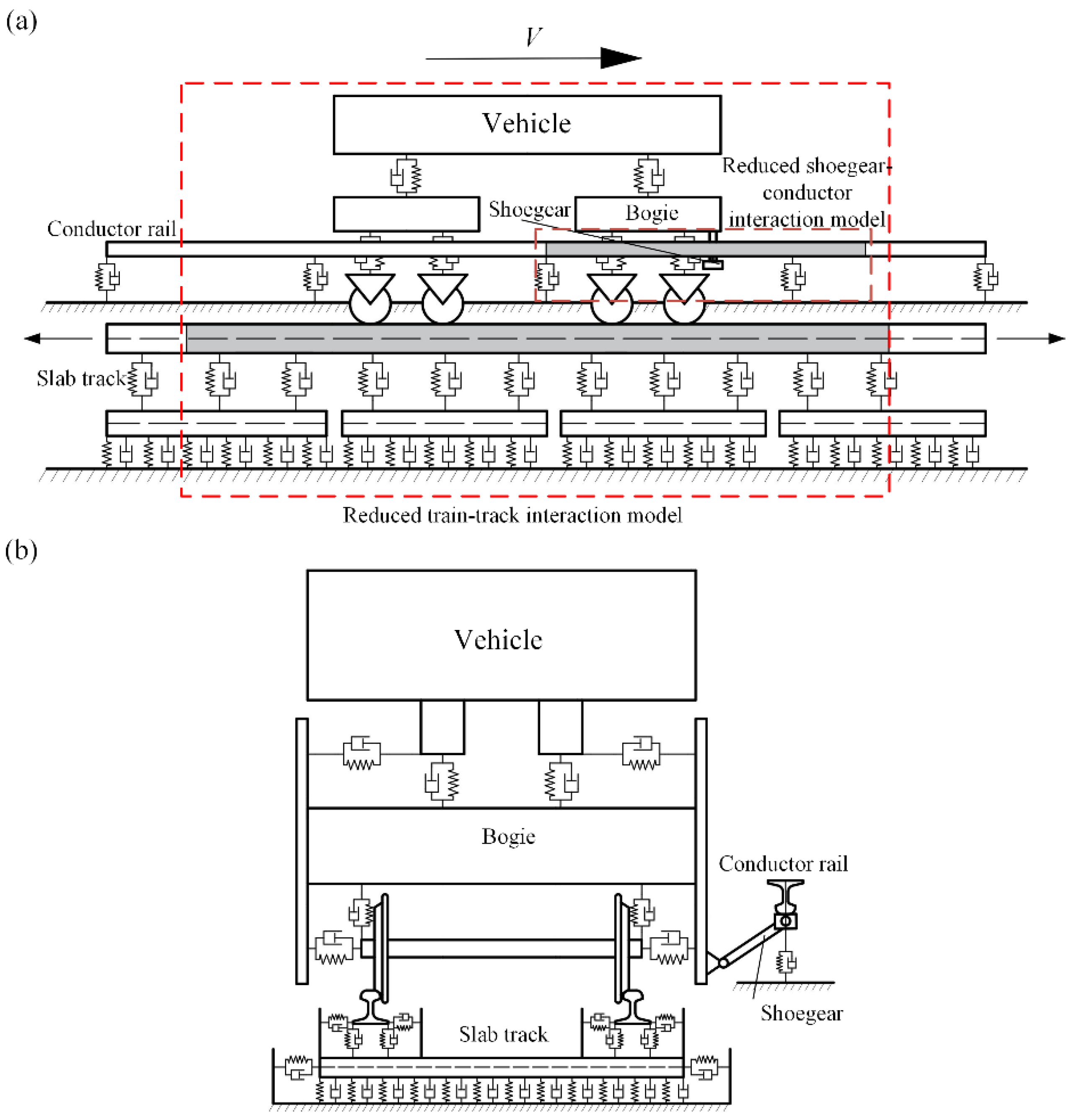
To address this issue, the present study compares the effects of track irregularity and conductor rail irregularity within a unified framework. A reduced collector shoe–conductor rail interaction model based on the reduced beam model (RBM) [12,13] is established and coupled in a one-way manner with an existing reduced train–track model [14]. As illustrated in Figure 1, only a local conductor rail region surrounding the moving collector shoe is retained. This local segment is described as a reduced conductor rail model by combining the Arbitrary Lagrangian–Eulerian (ALE) formulation with modal superposition. The reduced conductor rail and the moving collector shoe together form the shoe–rail subsystem. The previously developed RBM train–track model [14] provides the bogie frame vibration input, thereby yielding a reduced train–track–collector shoe–conductor rail model. Because both the long track and the long conductor rail are replaced by local moving submodels, the total number of DOFs is greatly reduced, and the simulation efficiency is improved. The reduced shoe–rail subsystem is validated against an existing MSM/FEM-based model [8], and the validated framework is then used to compare the influence of irregularities in the track and conductor rail. The remainder of the paper is organized as follows. Section 2 presents the train–track–collector shoe–conductor rail coupled model, Section 3 reports validation, Section 4 compares the influences of track and rail irregularities, and Section 5 summarizes the main findings.

2. Reduced Train–Track–Collector Shoe–Conductor Rail Coupled Model

In train–track interactions, the vibration induced by the moving train is mainly concentrated in a limited region surrounding the vehicle, and this region travels with the train owing to structural damping. This observation underlies both the moving element method (MEM) [15,16,17,18] and the RBM [12,13], where only the local active region rather than the entire track is retained while preserving good computational accuracy and efficiency. The conductor rail is also a damped structure; therefore, the same idea can be extended to collector shoe–conductor rail interactions. In this section, a reduced collector shoe–conductor rail model is first formulated. Note that the mass of the vehicle bogie can reach over ten tons, which is much higher than that of the collector shoe system. Moreover, the collector shoe–conductor rail contact force is usually smaller than 200 N, and its influence on the bogie dynamics can be ignored compared to the wheel–rail interaction and the carbody’s gravity. Therefore, only the influence of bogie vibration on collector shoe–conductor rail interaction needs to be considered, and the reduced collector shoe–conductor rail model is linked unidirectionally to the RBM-based reduced train–track model to build the coupled train–track–collector shoe–conductor rail model. The main modeling steps are described below.

2.1. Modeling of the Reduced Collector Shoe–Conductor Rail Interaction System

As noted above, the interaction between the collector shoe and the conductor rail mainly excites only a local region near the moving collector shoe. Consequently, this local segment can be modeled in place of the entire conductor rail, while its dynamic response is taken to represent the response of the full rail, as illustrated in Figure 2. This segment is referred to here as the reduced conductor rail model, and together with the moving collector shoe, it forms the reduced shoe–conductor rail subsystem. The reduced conductor rail translates with the collector shoe in the global coordinate system O-XYZ, whereas the collector shoe remains longitudinally fixed in the local coordinate system o-xyz attached to the reduced rail model. The subsystem, therefore, encounters different material portions of the conductor rail as time advances, which makes it a time-varying system. Small displacements and rotations are assumed for the reduced conductor rail.

2.1.1. The Reduced Conductor Rail Model

Based on ref. [8], the conductor rail is represented as an Euler–Bernoulli beam, and its supports are represented by stiffness-damping elements. Let l denote the length of the reduced conductor rail segment. The kinetic energy of this segment is written as:

$$T={\displaystyle \frac{1}{2}}{\displaystyle {\int }_0^l\rho A{\dot{y}}^{2}dx}+{\displaystyle \frac{1}{2}}{\displaystyle {\int }_0^l\rho A{\dot{z}}^{2}dx}+{\displaystyle \frac{1}{2}}{\displaystyle {\int }_0^l\rho \left(I_y+I_z\right){\dot{\varphi }}^{2}dx}$$

(1)

In this formulation, $\rho$ represents the density of the conductor rail, A denotes its cross-sectional area, and $I_y$ and $I_z$ are the second moments of area of the cross-section about the $y$- and $z$-axes, respectively. The generalized displacements $y$, $z$, and $\varphi$ correspond to the vertical, lateral, and torsional motions of the conductor rail cross-section, respectively. An overdot in Equation (1) denotes the derivative with respect to time. Similarly, the strain energy of the model is given by:

$$U={\displaystyle \frac{1}{2}}{\displaystyle {\int }_0^{l}E{I}_y}{\left(z^{″}\right)}^{2}dx+{\displaystyle \frac{1}{2}}{\displaystyle {\int }_0^{l}E{I}_z}{\left(y^{″}\right)}^{2}dx+{\displaystyle \frac{1}{2}}{\displaystyle {\int }_0^{l}G{I}_p}{\left({\varphi }^{″}\right)}^{2}dx$$

(2)

In this formulation, E represents the Young’s modulus of the conductor rail, G represents the shear modulus of the conductor rail, and I_P represents the torsional modulus of the conductor rail. In addition, ${\left(·\right)}^{\prime }$ denotes the partial derivative of the variable $\left(·\right)$ with respect to the coordinate x.

According to Equations (1) and (2), the displacements and rotations of the reduced conductor rail model can be further solved using the Galerkin method [19], as follows:

$$y\left(x,t\right)=Y\left(x\right)q_y\left(t\right),z\left(x,t\right)=Z\left(x\right)q_z\left(t\right),\varphi \left(x,t\right)=\Phi \left(x\right)q_{\theta x}\left(t\right)$$

(3)

In this formulation, $Y$, $Z$, and $\Phi$ denote the trial functions, while $q_y$, $q_z$, and $q_{\theta x}$ represent the vectors of the associated generalized coordinates. As mentioned above, the conductor rail vibration caused by the collector shoe–conductor rail interaction is mainly concentrated in a small region around the moving collector shoe due to the structure damping [13]. The conductor rail’s support provides damping to the conductor rail system. Therefore, at the boundary of this small region, the vibration amplitude is close to zero, which can be described as follows:

$$y\left(x,t\right)=0, z\left(x,t\right)=0, \varphi \left(x,t\right)=0$$

(4)

$$\dot{y}\left(x,t\right)=0, \dot{z}\left(x,t\right)=0, \dot{\varphi }\left(x,t\right)=0$$

(5)

where x_B is the boundary coordinate. Note that the boundary of this model is not a real boundary with a truncated beam, but is a moving boundary in the continuous beam with its vibration close to zero. Moreover, while both the simply supported and clamped–clamped boundary conditions can meet this situation, the shape function of the simply supported boundary condition is simple and can be easily applied in the dynamic equation derivation process. Therefore, the present model considers the simply supported boundary condition. The expression of these trail functions can be seen in [20].

As noted above, the present reduced conductor rail model is a time-varying system. Therefore, the variable x in Equations (1) and (2) is also a function of both the global coordinate of the material point in the O-XYZ frame and time t, which can be written as [20]:

$$x=f\left(X,t\right)=X-d\left(t\right)=X-Vt$$

(6)

In this formulation, d(t) is the distance from the origin of O-XYZ to the origin of o-xyz, and V is the collector shoe speed. By applying the ALE formulation [21] to Equations (4) and (5) and then to Equations (1) and (2), the following relations are obtained [20]:

$$\dot{y}=-V{Y}^{\prime }{q}_y+Y{\dot{q}}_y, \dot{z}=-V{Z}^{\prime }{q}_z+Z{\dot{q}}_z, \dot{\varphi }=-V{\Phi }^{\prime }{q}_{\theta x}+\Phi {\dot{q}}_{\theta x}$$

(7)

$$y^{\prime }=Y^{\prime }{q}_y, z^{\prime }=Z^{\prime }{q}_z, {\varphi }^{\prime }={\Phi }^{\prime }{q}_{\theta x}$$

(8)

Substituting Equations (7) and (8) into Equations (1) and (2) and applying Lagrange’s equation yields the governing equations of the reduced conductor rail model as

$$M\ddot{q}+C\dot{q}+Kq=Q_{flow}+Q_F$$

(9)

In this formulation, $M$, $C$, and $K$ are the mass, damping, and stiffness matrices, respectively. $Q_{flow}$ is the additional generalized-force vector introduced by the relative motion between the reduced model and the conductor rail material, while $Q_F$ collects the generalized forces generated by external actions such as the shoe–rail contact force and support reactions. Expressions for $Q_{flow}$ are identical to those reported in ref. [9], and the derivation of $Q_F$ is provided in ref. [19]. In Equation (9), $q={\left[q_y,q_z,q_{\theta x}\right]}^T$. The matrices $M$, $C$, and $K$ are written as follows:

$$M=\left[\begin{array}{lll}\rho A{\displaystyle {\int }_0^l\left(Y^{T}Y\right)dx}& & \\ & \rho A{\displaystyle {\int }_0^l\left(Z^{T}Z\right)dx}& \\ & & \rho \left(I_y+I_z\right){\displaystyle {\int }_0^l\left({\Phi }^T\Phi \right)dx}\end{array}\right]$$

(10)

$$C=\left[\begin{array}{lll}-2\rho AV{\displaystyle {\int }_0^l\left(Y^T{Y}^{\prime }\right)}dx& & \\ & -2\rho AV{\displaystyle {\int }_0^l\left(Z^T{Z}^{\prime }\right)dx}& \\ & & -2\rho \left(I_y+I_z\right)V{\displaystyle {\int }_0^l\left({\Phi }^T\Phi \right)dx}\end{array}\right]$$

(11)

$$K=\left[\begin{array}{ccc}{K}_y& & \\ & K_z& \\ & & K_{\varphi }\end{array}\right]$$

(12)

In Equation (10), there are

$$K_y=\rho A{V}^2{\displaystyle {\int }_0^l\left(Y^T{Y}^{″}\right)}dx+E{I}_z{\displaystyle {\int }_0^l\left({Y^{″}}^T{Y}^{″}\right)}dx$$

(13)

$$K_z=\rho A{V}^2{\displaystyle {\int }_0^l\left(Z^T{Z}^{″}\right)}dx+E{I}_y{\displaystyle {\int }_0^l\left({Z^{″}}^T{Z}^{″}\right)}dx$$

(14)

$$K_{\varphi }=\rho A{V}^2{\displaystyle {\int }_0^l\left({\Phi }^T{\Phi }^{″}\right)}dx+G{I}_p{\displaystyle {\int }_0^l\left({{\Phi }^{\prime }}^T{\Phi }^{\prime }\right)}dx$$

(15)

The support of the conductor rail is considered as a spring-damper element, and its corresponding force can be calculated by

$$F_{di}=K_S{d}_{Si}+C_S{\dot{d}}_{Si}$$

(16)

where $d_{Si}$ is the displacement of the conductor rail at the support location. Notably, the position of the ith support $x_{di}$ at any time can be expressed as

$$x_{di}=x_{d0i}-Vt$$

(17)

In addition, only the supports satisfying $0\le x_{di}\le l$ are included in the reduced conductor rail model. In the present model, its accuracy is decided by its length. As mentioned above, the model length should be long enough to allow the vibration at its boundary to be close to zero. If the length of the model is not long enough, the vibration at the boundary is not close to zero, and the simply supported boundary condition does not meet the real situation. This will obviously cause an error in the results.

2.1.2. Collector Shoe Model

The collector shoe is then modeled, where the main part of the collector shoe is modeled as a rotating rigid body, and the contact strip at its top is treated as a lumped mass. According to ref. [22], the dynamic equation of the collector shoe can be written as

$$\left({\displaystyle \frac{1}{3}}m{l}^2+m_2{l}_2^2\right)\ddot{\theta }+C\dot{\theta }+K\theta =\left(F_c-F_0\right)l_2+\left({\displaystyle \frac{1}{2}}ml+m_2{l}_2\right){\ddot{u}}_z$$

(18)

In this formulation, m is the collector shoe mass and m₂ is the mass of the contact strip. The quantity l is the collector shoe length, and l₂ is the distance between the rotation shaft and the contact strip. C and K denote the torsional damping and stiffness, respectively. $\theta$ is the rotation angle of the collector shoe, and ${\ddot{u}}_z$ is the bogie acceleration at the collector shoe seat. $F_c$ is the collector shoe–conductor rail rail contact force, and $F_0$ is the initial force acting on the collector shoe. The $F_c$ is calculated by

$$F_c=\left\{\begin{array}{c}{k}_n{d}_r,d_r\ge 0\\ 0,d_r<0\end{array}\right.$$

(19)

In this equation, $k_n$ denotes the contact stiffness and is taken as 50,000 N/m [8], while $d_r$ represents the gap between the contact strip and the conductor rail, in which the irregularity of the conductor rail is also included.

2.1.3. Governing Equations of the Reduced Collector Shoe–Conductor Rail Subsystem

Combining the equations of the reduced conductor rail model with those of the collector shoe gives the dynamic equations of the reduced collector shoe–conductor rail subsystem as

$$\begin{array}{l}\left[\begin{array}{ll}M& \\ & \left({\displaystyle \frac{1}{3}}m{l}^2+m_2{l}_2^2\right)\end{array}\right]\left[\begin{array}{c}\ddot{q}\\ \ddot{\theta }\end{array}\right]+\left[\begin{array}{cc}C& \\ & C\end{array}\right]\left[\begin{array}{c}\dot{q}\\ \dot{\theta }\end{array}\right]\\ +\left[\begin{array}{cc}K& \\ & K\end{array}\right]\left[\begin{array}{c}q\\ \theta \end{array}\right]=\left[\begin{array}{c}{Q}_{flowm}+Q_F\\ \left(F_c-F_0\right)l_2+\left({\displaystyle \frac{1}{2}}ml+m_2{l}_2\right){\ddot{u}}_z\end{array}\right]\end{array}$$

(20)

In the present model, the collector shoe is considered as a rigid body, and the real cross-section shape of the conductor rail is not considered. This results in the ignorance of high-frequency acoustic, impact-related phenomena, or a lack of high-frequency oscillations in the contact force. While the contact force’s accuracy is dominated by low-frequency parts, and its accuracy is not influenced by this, it will be further solved through modeling the conductor rail and collector shoe based on the FEM method.

2.2. Model of the RBM-Based Train–Track Interaction Model

The RBM-based train–track interaction model is next introduced. The vehicle is taken as a subway car and the track as a ballastless track, which is widely used in metro systems. The vehicle is modeled as a multibody system, whereas the ballastless track includes rails, fastenings, slabs, and cement–asphalt (CA) mortar layers. Within the RBM framework, the long ballastless track is reduced to a local region around the vehicle, so that only the slabs lying in that region need to be retained. Full details of the RBM-based train–track model are given in ref. [14], and its governing equation is [14].

$$\left[\begin{array}{cc}{M}_V& \\ & M_T\end{array}\right]\left[\begin{array}{c}{\ddot{q}}_V\\ {\ddot{q}}_T\end{array}\right]+\left[\begin{array}{cc}{C}_V& \\ & C_T\end{array}\right]\left[\begin{array}{c}{\dot{q}}_V\\ {\dot{q}}_T\end{array}\right]+\left[\begin{array}{cc}{K}_V& \\ & K_T\end{array}\right]\left[\begin{array}{c}{q}_V\\ q_T\end{array}\right]=\left[\begin{array}{c}{Q}_V\\ Q_T\end{array}\right]$$

(21)

In this formulation, $M$, $C$, and $K$ denote the mass, damping, and stiffness matrices. Subscripts V and T refer to the vehicle and track subsystems, respectively. $Q_V$ is the generalized-force vector produced by vehicle gravity and wheel–rail contact forces, whereas $Q_T$ is the generalized-force vector of the ballastless track generated by the same wheel–rail contact forces. Detailed matrix expressions are provided in ref. [11].

The wheel–rail contact formulation is summarized here for completeness. The normal contact force is computed using Hertzian nonlinear contact theory [23], and the creep force is evaluated with the Shen–Hedrick–Elkins model [16]. Additional details of the wheel–rail contact algorithm are given in ref. [24], where the effect of track irregularity is also incorporated.

2.3. The Reduced Train–Track–Collector Shoe–Conductor Rail Interaction Model

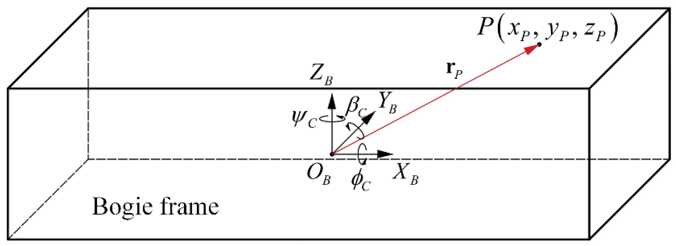
Based on the reduced collector shoe–conductor rail and RBM-based train–track interaction model, the reduced train–track–collector shoe–conductor rail model can be finally formulated, as shown in Figure 1. The coupling between the reduced collector shoe–conductor rail model and the RBM-based train–track interaction model is achieved through the transmission of the vertical acceleration of the bogie frame at the collector shoe seat. The pantograph mounting point on the bogie frame is denoted by P, and the reference coordinate system of the bogie frame is defined as O_B-X_BY_BZ_B. In addition, as shown in Figure 3, the position vector of point $P$ can be written as r_P= [x_p, y_p, z_p]. Accordingly, the displacement vector of point P can be further expressed as

$$r_{dP}=r_{dC}+{\tilde{\Psi }}_C{r}_P=\left[\begin{array}{c}0\\ y_C\\ z_C\end{array}\right]+\left[\begin{array}{ccc}0& -{\psi }_C& {\beta }_C\\ {\psi }_C& 0& -{\varphi }_C\\ -{\beta }_C& {\varphi }_C& 0\end{array}\right]\left[\begin{array}{c}{x}_P\\ y_P\\ z_P\end{array}\right]=\left[\begin{array}{c}-y_P{\psi }_C+z_P{\beta }_C\\ y_C+x_P{\psi }_C-z_P{\varphi }_C\\ z_C-x_P{\beta }_C+y_P{\varphi }_C\end{array}\right]$$

(22)

In this formulation, ${\varphi }_C$, ${\beta }_C$, and ${\psi }_C$ are the roll, pitch, and yaw angles of the bogie frame, respectively. The variables y_C and z_C represent the lateral and vertical displacements of the centroid of the bogie frame in the global coordinate system. According to Equation (22), the vertical displacement of the bogie frame at point P can be expressed as

$$u_{PZ}=z_C-x_P{\beta }_C+y_P{\varphi }_C$$

(23)

and the corresponding vertical acceleration at point P is

$${\ddot{u}}_{PZ}={\ddot{z}}_C-x_P{\ddot{\beta }}_C+y_P{\ddot{\varphi }}_C$$

(24)

It should be noted that the mass of the collector shoe is negligible in comparison with that of the bogie frame. Therefore, the vertical acceleration at the collector shoe seat on the bogie frame is first determined by solving Equation (21), and the resulting acceleration is then introduced into Equation (20) to investigate the effect of train–track interaction on the dynamic interaction between the collector shoe and the conductor rail. In this study, the commercial software MATLAB 2022a is employed to implement Equations (20) and (21), which are solved using a variable-step, variable-order (VSVO) algorithm through the MATLAB function ode15s.

3. Validation

After the formulation of the reduced train–track–collector shoe–conductor rail model, its accuracy and computational efficiency are evaluated. It should be noted that the RBM-based reduced train–track interaction model has already been validated in ref. [14]. Therefore, the present section mainly focuses on the validation of the reduced collector shoe–conductor rail interaction system. To this end, the proposed model is compared with an existing collector shoe–conductor rail interaction model established based on the finite element method (FEM), which was developed by Song et al. [8] and validated against experimental results. Note that the measurement data validation is not considered here due to the limitations of funding and the metro operation company, which further limited the line or bench test.

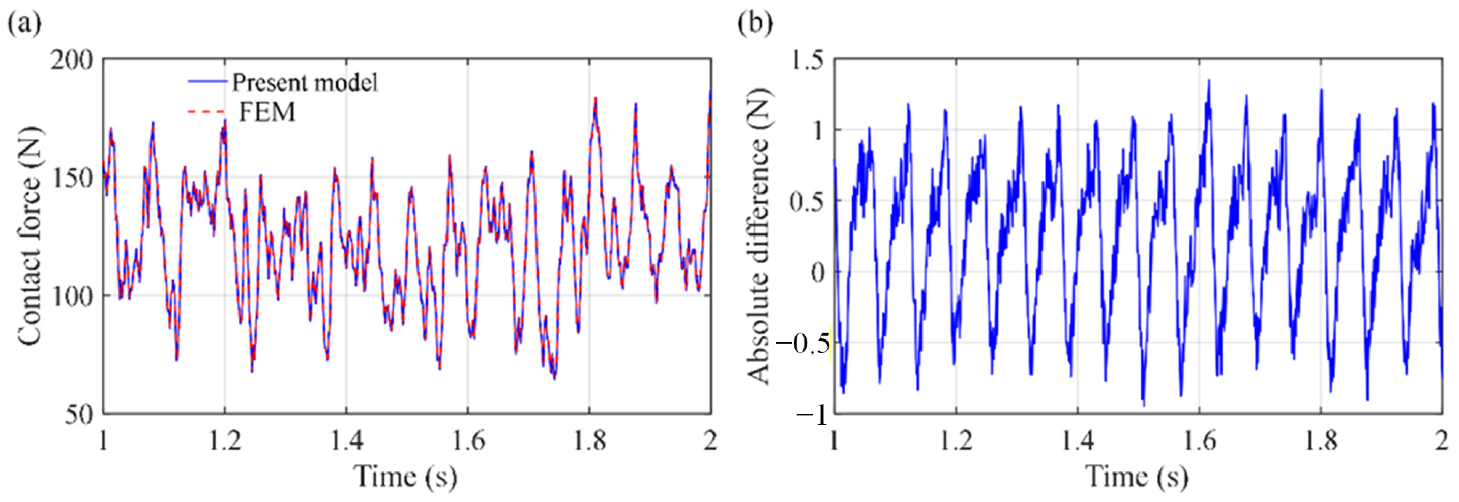
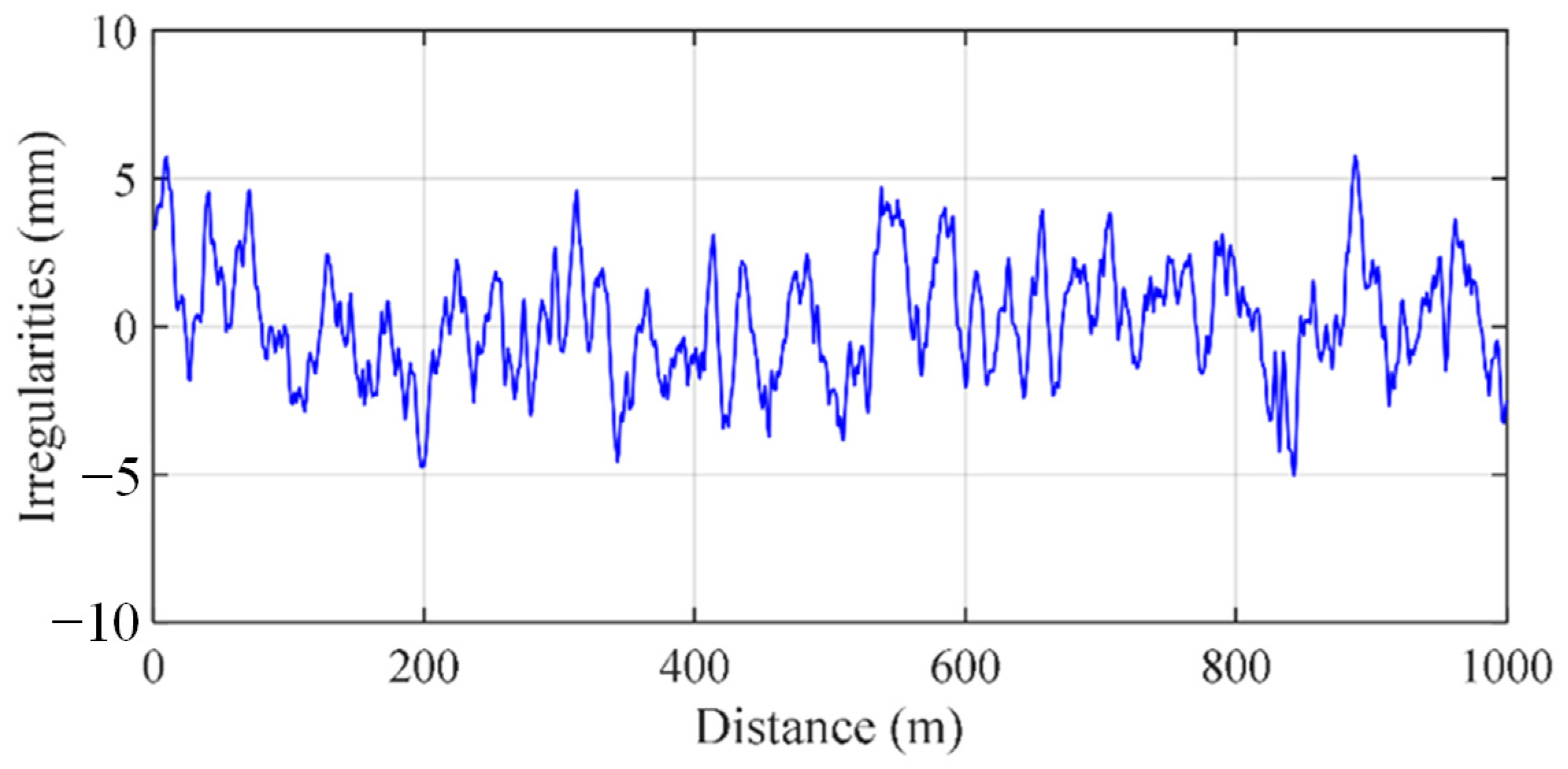
A collector shoe–conductor rail interaction system in the Beijing subway is taken as the case study. The total length of the conductor rail is 1200 m, while the length of the reduced conductor rail is set to 60 m in the present analysis. In the proposed model, the number of modes is taken as $n=60$, whereas 2400 beam elements are adopted in the FEM model. The vehicle operating speed is 120 km/h. The time histories of the collector shoe–conductor rail contact force are presented in Figure 4, where the results obtained from the present model are compared with those from the FEM model. In addition, the conductor rail irregularity derived from measured data is incorporated into the calculation, as illustrated in Figure 5. As can be observed from Figure 4, the results predicted by the present model agree well with those of the FEM model, with the maximum absolute difference not exceeding 1.45 N and the corresponding relative difference being less than 2.6%. These results demonstrate the accuracy of the proposed reduced collector shoe–conductor rail interaction model.

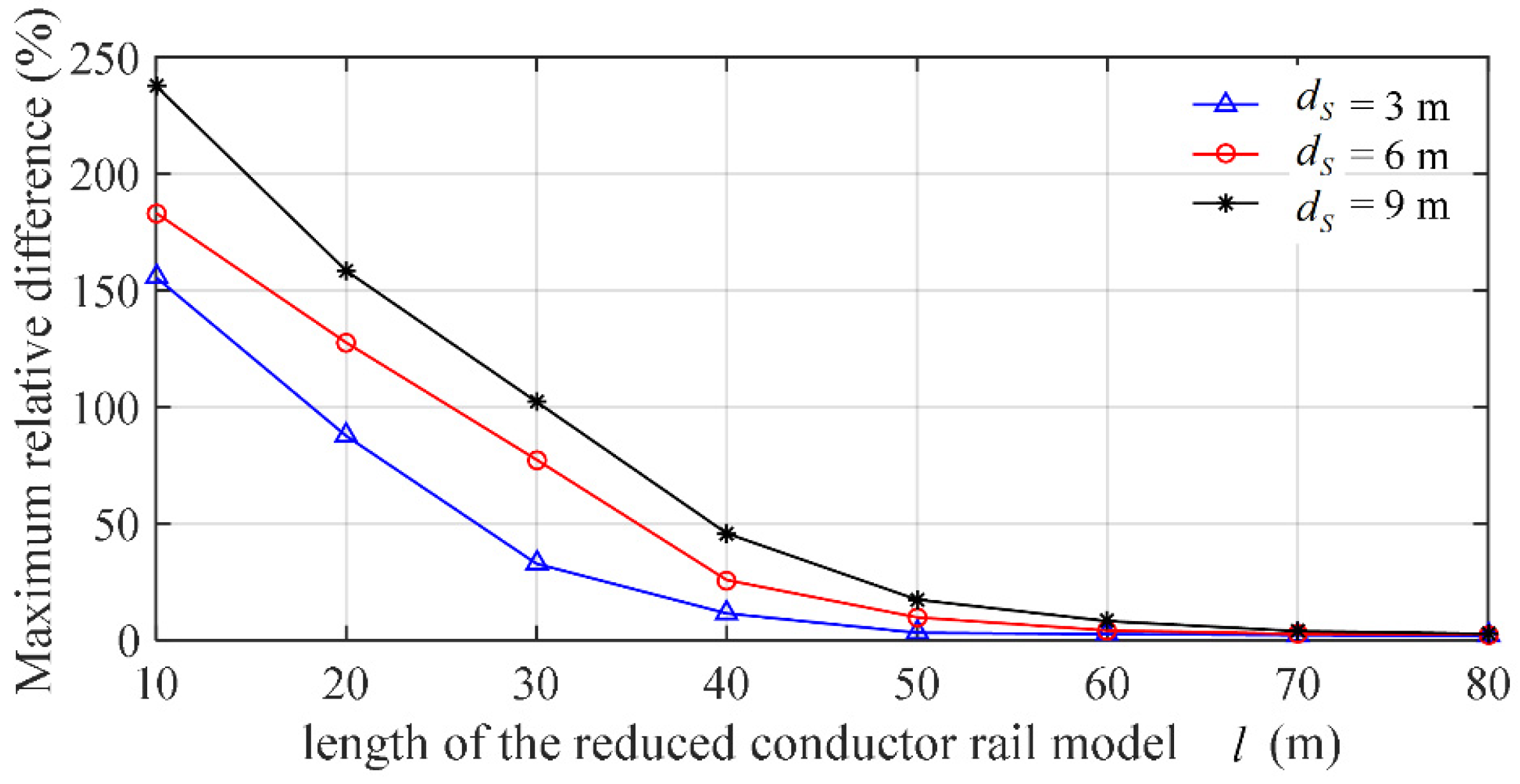
As noted above, the length of the reduced conductor rail model, $l$, should be sufficiently large to capture most of the vibration response of the conductor rail. Otherwise, part of the conductor rail vibration will be excluded from the reduced model, thereby reducing the accuracy of the reduced collector shoe–conductor rail interaction model. Accordingly, the effect of the reduced conductor rail length $l$ on the accuracy of the present model is further examined in this section. It should be emphasized that the structural damping of the conductor rail increases with the number of supports, which is determined by the spacing between adjacent supports. Therefore, the support spacing, $d_S$, also affects the appropriate choice of $l$ and is considered in the present analysis. The maximum relative difference between the present model and the FEM model for different values of $l$ and $d_S$ is presented in Figure 6. As shown in Figure 6, the maximum relative difference between the present model and the FEM model decreases as $l$ increases, whereas it increases with increasing $d_S$. When d_S = 3 m, the maximum relative difference decreases to 3.2% with l equal to 50 m, and it remains smaller than 3% with l larger than 50 m. However, when d_S = 9 m, the maximum relative difference increases to 9.8% with l equal to 50 m, and it becomes smaller than 5% with l larger than 70 m. Because the d_S is equal to 3 m in the present case, the present model can obtain accurate results with l equal to 60 m. Note that the l is decided by the vibration wave transmission velocity, and it is further decided by the structural parameters, especially the damping. These factors are highly nonlinear and hard to express by a single formula. Therefore, the appropriate value of l should also be individually decided in different collector shoe–conductor rail interaction cases.

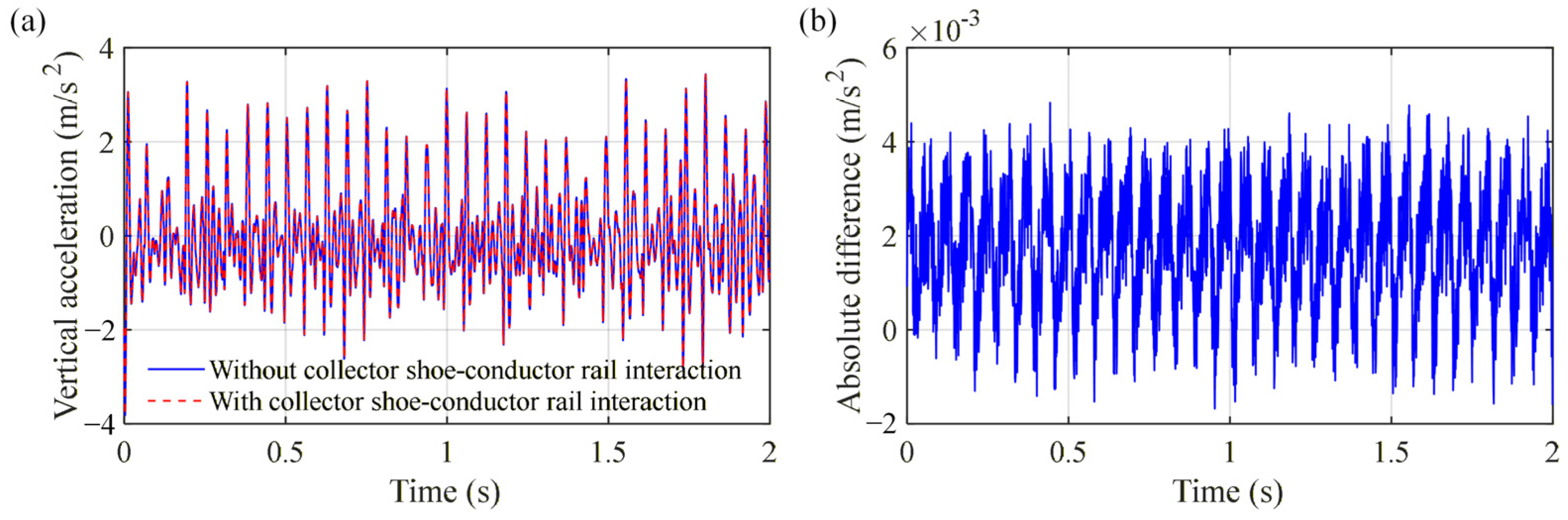
As mentioned above, the influence of the collector shoe–conductor rail interaction on the bogie dynamics can be ignored due to the mass difference. This phenomenon should be further validated to ensure the model’s accuracy. Based on the present validation case, the bogie vertical acceleration with and without the influence of collector shoe–conductor rail interaction is shown in Figure 7. It can be seen from Figure 7 that the influence of collector shoe–conductor rail interaction on bogie vertical acceleration can be ignored, where the maximum absolute difference is no more than 0.005 m/s². Moreover, the present bogie’s vibration will only be obviously influenced by a maximum collector shoe–conductor rail contact force higher than 2000 N, which is a kind of extreme condition. Based on these results, the present phenomenon is further validated.

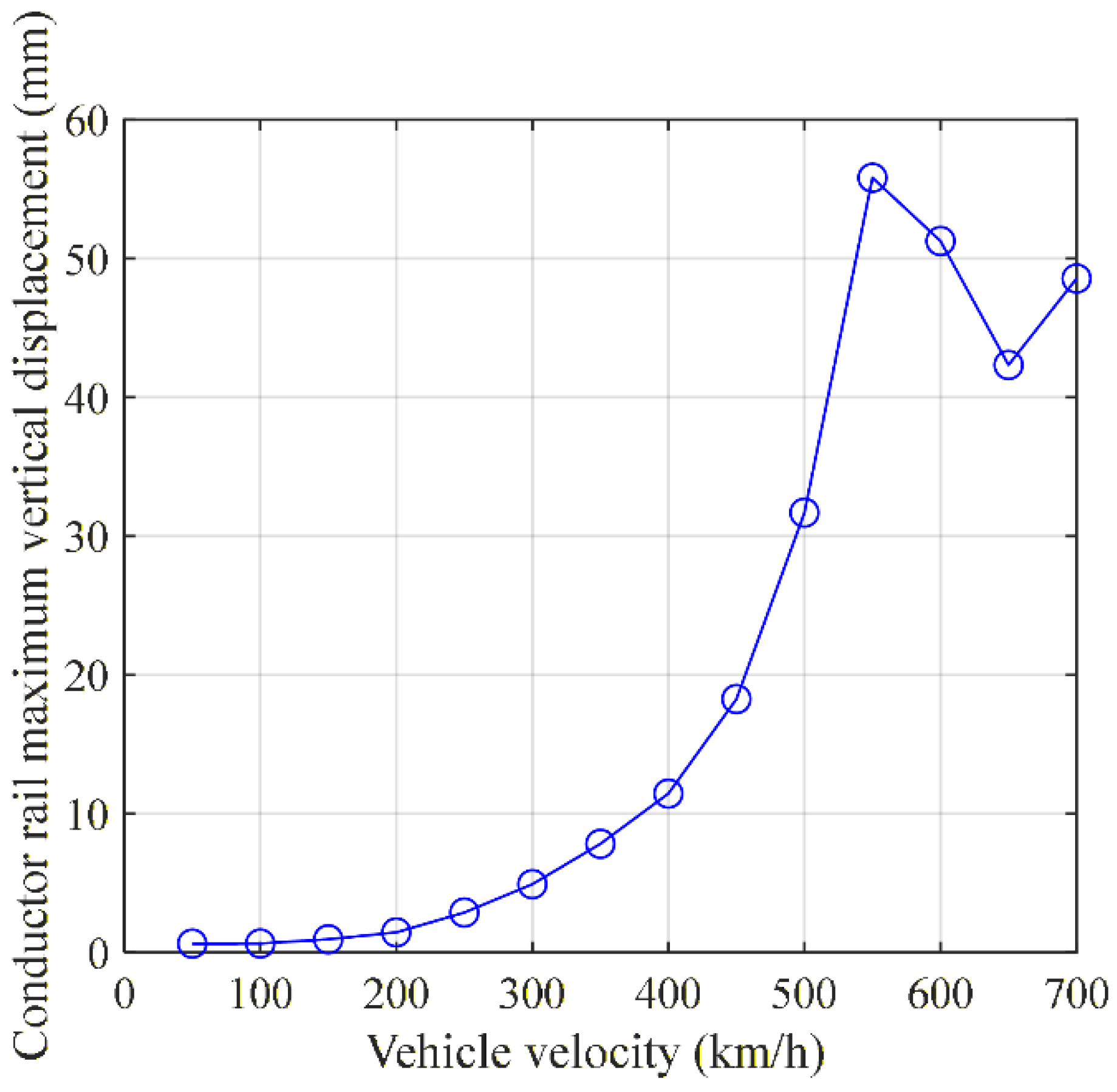
The model’s small-displacement assumption under different vehicle speeds is then validated. The conductor rail’s maximum vertical displacement at the contact point corresponding to different vehicle speeds is shown in Figure 8. It can be seen from Figure 8 that the trend of the contact rail’s maximum vertical displacement changes at V = 550 km/h, and the nonlinear geometric effects show at this point. Therefore, the vehicle speed larger than 550 km/h makes the small-displacement assumption invalid. Note that this speed is much higher than the metro vehicle’s maximum operation speed, which means that the small-displacement assumption is valid in the metro vehicle system.

The computational efficiency of the proposed reduced collector shoe–conductor rail interaction model is further evaluated in this section. Based on the validation case described above, the number of degrees of freedom (DOFs) and the computational times of the conventional FEM model and the present model are compared. The train operating speed remains 120 km/h, and the simulation duration is 30 s, corresponding to an operating distance of 1000 m. As noted previously, in the conventional model, the conductor rail length is 1200 m, and the total number of DOFs is 7204. In contrast, in the present model, the length of the reduced conductor rail system is only 60 m, with a total of 181 DOFs. The corresponding computational times for the conventional model and the present model are 1839 s and 332 s, respectively, indicating that the proposed model is approximately six times faster than the traditional FEM under long-distance operating conditions. Moreover, since the existing RBM-based reduced train–track interaction model has also been shown to be more computationally efficient than the MSM [14], the present reduced train–track–collector shoe–conductor rail model is capable of efficiently predicting collector shoe–conductor rail interactions under the influence of train–track interaction, in comparison with the traditional approach.

4. Comparison Study on the Influence of Track and Conductor Rail Irregularity on Collector Shoe–Conductor Rail Interaction Dynamics

Based on the present reduced train–track–collector shoe–conductor rail interaction model, the influence of track and conductor rail’s irregularity on collector shoe–conductor rail interaction dynamics is investigated and compared with each other. Both the track irregularity and the conductor rail irregularity presented in Figure 5 are fully taken into account in the train–track interaction system. The parameters of the train–track system and the collector shoe–conductor rail system are selected based on those of the Beijing subway system. The vehicle operating speed is set to 120 km/h, which corresponds to the maximum design speed of the new subway line. The length of the reduced conductor rail model, $l$, is taken as 60 m, while the length of the reduced track model is 52.8 m.

4.1. Basic Influence

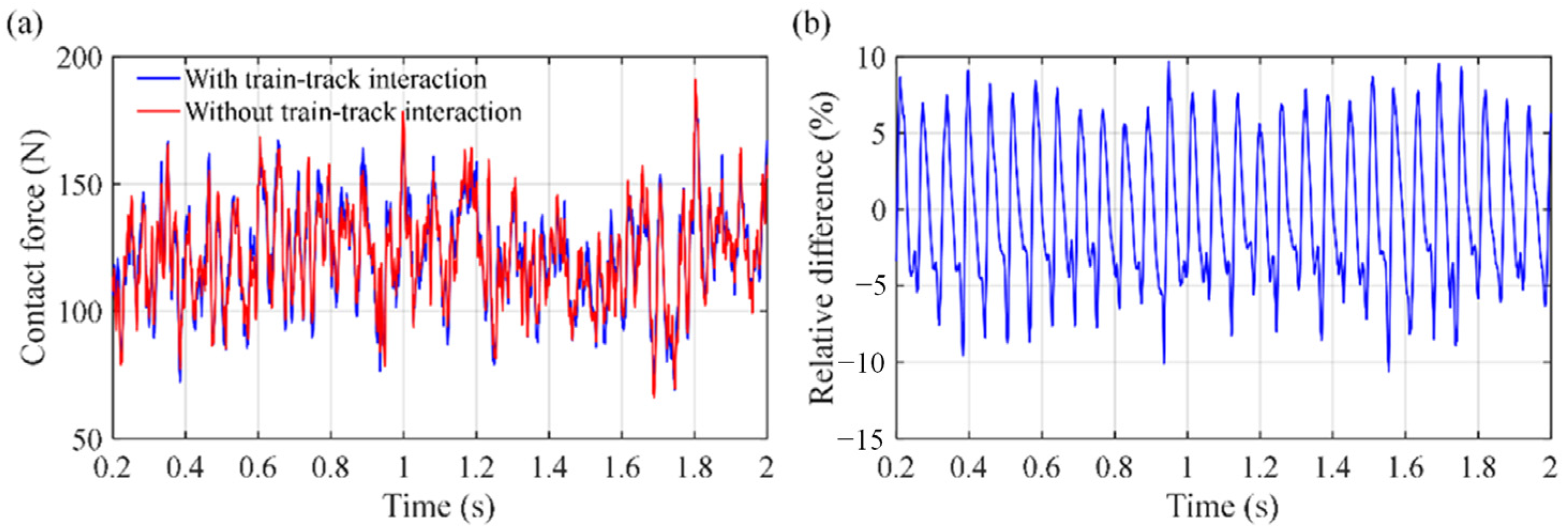
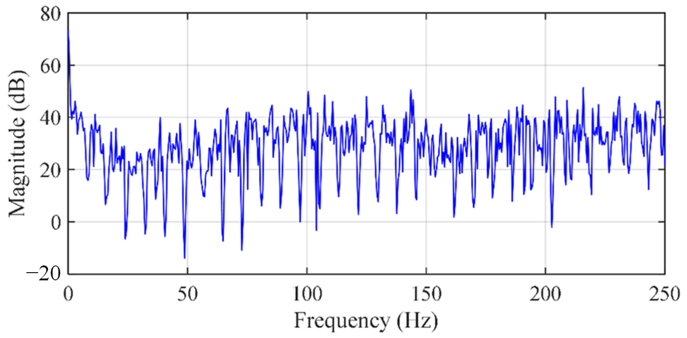
The influence of train–track interaction on collector shoe–conductor rail interaction dynamics with normal track irregularities is first investigated. The time histories of the collector shoe–conductor rail contact force with and without the influence of train–track interaction are shown in Figure 9, and the estimated transfer function between the bogie vibration and collector shoe–conductor rail contact force is shown in Figure 10. It can be seen from Figure 9 that the train–track interaction does have some influence on collector shoe–conductor rail interaction dynamics, but this influence is not obvious, even with the highest vehicle operation velocity and only concentrates in a specific frequency domain. The maximum relative difference between the results with and without train–track interaction is no more than 10% but larger than 5%, and it mainly happens in the 0–100 Hz frequency domain. This means that ignoring the influence of train–track interaction can result in inaccurate results of the collector shoe–conductor rail interaction dynamic responses, especially in the low-frequency domain.

4.2. Comparison Between the Influence of Different Key Factors on Collector Shoe–Conductor Rail Interaction Dynamics

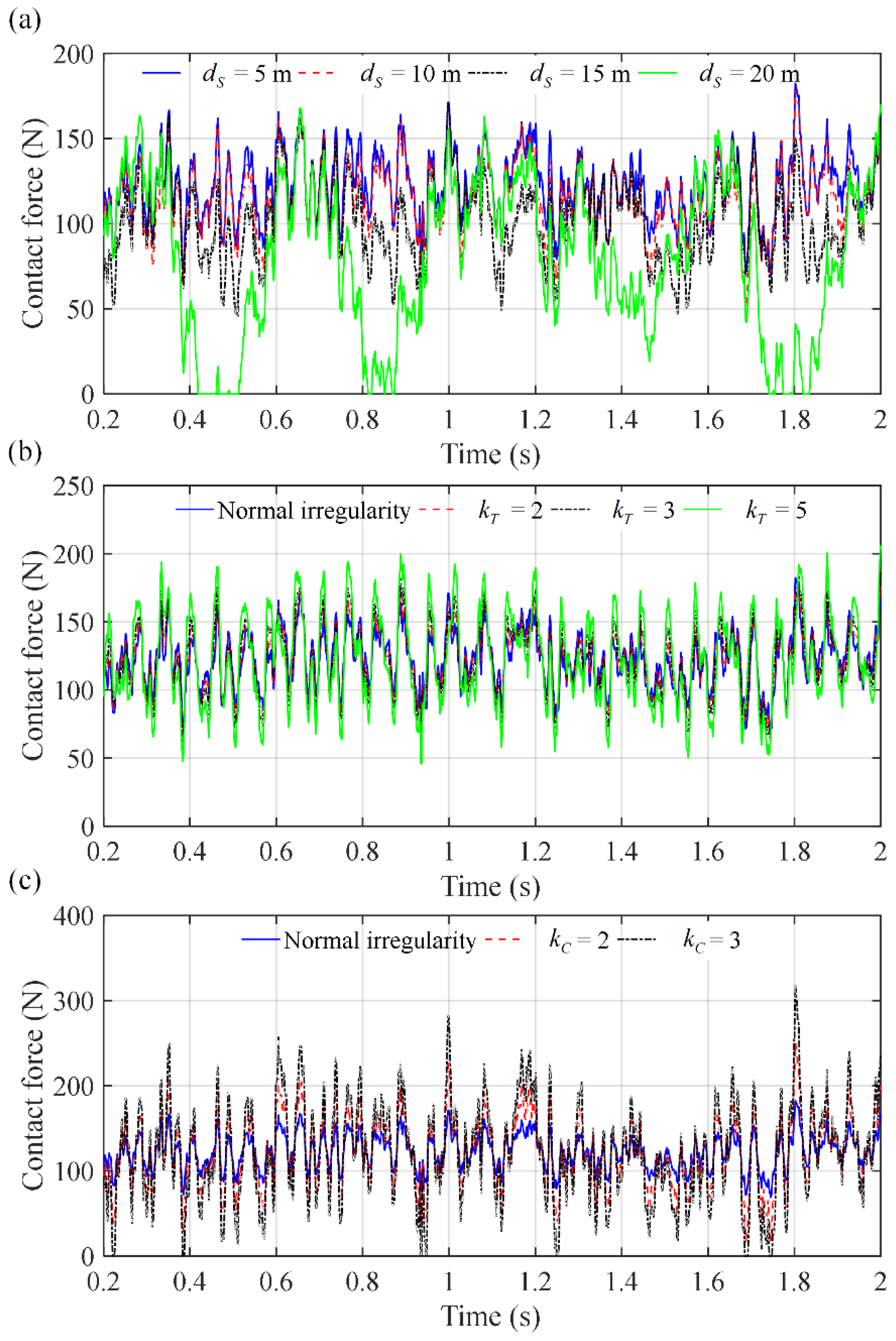
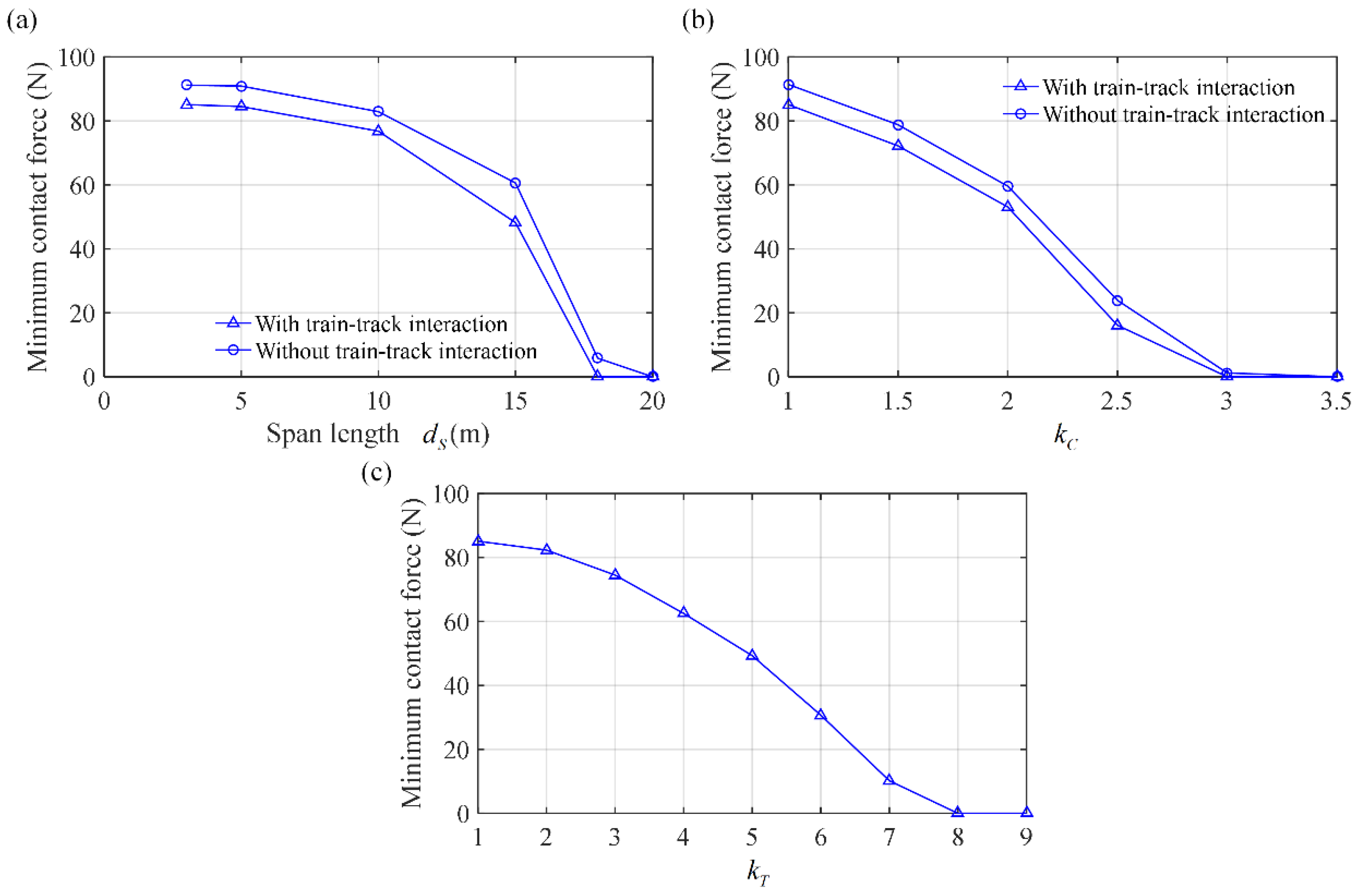
As mentioned above, the conductor rail irregularity and support distance has direct influence on collector shoe–conductor rail interaction dynamics, and their influence is further calculated and compared with that of the train–track interaction. With different support distance d_S, conductor rail irregularity, and track irregularity considered, their corresponding collector shoe–conductor rail contact forces are calculated first, as shown in Figure 11, where k_T is the ratio between different track irregularities and normal track irregularity’s amplitude, and k_C is the ratio between different conductor rail irregularities and normal conductor rail irregularity’s amplitude. The minimum collector shoe–conductor rail contact force, with respect to different d_S, k_T, and k_C, is shown in Figure 12. It can be seen from Figure 11 and Figure 12 that the conductor rail irregularities and support distance have a much stronger influence than that of the track irregularity. When d_S is larger than 17.5 m or k_C is larger than 3, the minimum collector shoe–conductor rail contact force is decreased to zero, and it becomes more unstable when they are close to these values. But it only becomes 0 with k_T larger than 8. When k_T is 5, the dynamic responses of the collector shoe–conductor rail interaction are still stable. The train–track interaction also has a small influence with different d_S and k_C, where the minimum contact force only decreases to 10 N when a train–track interaction is considered. Because a track irregularity with its amplitude eight times larger than normal irregularity has an obvious influence on train–track interaction and can even cause unstable behavior of the train, it is difficult for the train–track interaction to heavily influence collector shoe–conductor rail interaction dynamics, and the conductor rail’s irregularity has a stronger influence, similarly.

5. Conclusions

In this study, the effects of track irregularity and conductor rail irregularity on the collector shoe–conductor rail interaction dynamics are investigated and systematically compared. To accurately and efficiently analyze these effects, a reduced train–track–collector shoe–conductor rail interaction model is developed. In the proposed model, the conductor rail is reduced to a limited region surrounding the moving collector shoe, and this local region is modeled as a reduced conductor rail system. Together with the collector shoe, the reduced conductor rail model constitutes the reduced collector shoe–conductor rail interaction model. Since the reduced conductor rail model moves synchronously with the collector shoe and represents different portions of the conductor rail structure over time, it is inherently a time-varying system. Accordingly, the arbitrary Lagrangian–Eulerian (ALE) formulation and the modal superposition method (MSM) are employed to establish its governing dynamic equations. Furthermore, the existing RBM-based reduced train–track interaction model is unidirectionally coupled with the reduced collector shoe–conductor rail interaction model to formulate the reduced track–train–collector shoe–conductor rail interaction model, in which the calculated bogie vibration response is transmitted to the reduced collector shoe–conductor rail interaction system. By reducing both the long track and the conductor rail, the total number of degrees of freedom of the overall train–track–collector shoe–conductor rail interaction model is significantly decreased, thereby improving computational efficiency. After validation, the proposed model is applied to investigate the respective influences of track irregularity and conductor rail irregularity on the collector shoe–conductor rail interaction system in the Beijing subway, and a comparative analysis of these two effects is subsequently conducted.

According to the results, the present reduced collector shoe–conductor rail interaction model can accurately and efficiently calculate the dynamic response of the collector shoe–conductor rail interaction, where its calculation time can reach six times faster than the traditional FEM in a long travel distance situation. In the subway system, the track irregularity does have some influence on collector shoe–conductor rail interaction dynamics, but this influence is limited to no more than 10% compared to that of the conductor rail’s irregularity. The conductor rail irregularity and support distance have a much stronger influence than the track irregularity, and the conductor rail can even cause contact loss in certain conditions, when its irregularity amplitude becomes twice higher than normal irregularity. Therefore, both factors must be integrated into future studies of collector shoe–conductor rail dynamics, and the conductor rail’s irregularity must be considered to maintain its condition.

In our next studies, the present model will be further upgraded with a flexible collector shoe and a detailed conductor rail model. The long-term component wear and fatigue problem will be concentrated and solved, and the line test will also be conducted to provide measurement data.

References

1. Hartland, D.J. High-Speed Third Rail Collector shoe. Proc. Inst. Mech. Eng. F J. Rail Rapid Transit. 1995, 209, 77–85. [Google Scholar] [CrossRef] [Scilit]
2. Dong, L.; Chen, G.X.; Zhu, M.H.; Zhou, Z. Wear mechanism of aluminum–stainless steel composite conductor rail sliding against collector shoe with electric current. Wear 2007, 263, 598–603. [Google Scholar] [CrossRef] [Scilit]
3. Stewart, E.; Weston, P.; Hillmansen, S.; Roberts, C. Using bogie-mounted sensors to understand the dynamics of third rail current collection systems. Proc. Inst. Mech. Eng. F J. Rail Rapid Transit 2011, 225, 219–227. [Google Scholar] [CrossRef] [Scilit]
4. Weston, P.F.; Stewart, E.; Roberts, C.; Hillmansen, S. Measuring the dynamic interaction between electric vehicle collector shoe and the third rail. In 2008 International Conference on Railway Engineering-Challenges for Railway Transportation in Information Age; IET: Hong Kong, China, 2008; pp. 1–4. [Google Scholar]
5. Paudel, M.; Lim, L.J.; Yap, F.F.; Kho, K. Vibration analysis of the third rail structure of a mass rapid transit system with structural defects. Appl. Sci. 2021, 11, 8410. [Google Scholar] [CrossRef] [Scilit]
6. Jinfa, G.; Jiqin, W.; Yuan, Z. Dynamics analysis of electric collector shoe and conductor rail system. J. Vibroeng. 2014, 16, 1992–2007. [Google Scholar]
7. Meng, H.; Wei, X.; Liu, Y. Study on Dynamic Characteristics and Improvement of the Current Collector in High-speed Metro Vehicles. In 2018 International Conference on Mechanical, Electrical, Electronic Engineering & Science (MEEES 2018); Atlantis Press: Dordrecht, The Netherlands, 2018; pp. 476–481. [Google Scholar]
8. Wang, X.; Liu, Z.; Song, Y.; Jin, W.; Xu, Z.; Xiong, J.; Zhou, S. Dynamic Characteristics of Electric Collector shoe and Conductor Rail System Considering the Track Irregularities. IEEE Trans. Instrum. Meas. 2023, 72, 1–13. [Google Scholar]
9. Erdoğan, Ş.; Usta, Y. Sliding movement temperature analysis between composite conductor rail and a collector shoe. Proc. Inst. Mech. Eng. Part F J. Rail Rapid Transit 2023, 237, 541–550. [Google Scholar] [CrossRef] [Scilit]
10. Pan, L.; Peng, P.; Xing, T.; Yang, C.; He, F. Effects of train speed on dynamic performance of shoe-rail interaction system. Adv. Mech. Eng. 2024, 16, 16878132241239799. [Google Scholar] [CrossRef] [Scilit]
11. Chen, Y.; Liu, X.; Hatem, M.; Zhou, K.; Ji, Y. Monitoring Carbon Slide Wear in Metro Train Current Collector Shoes Using 3-D Point Cloud Data. IEEE Sens. J. 2025, 26, 2373–2380. [Google Scholar] [CrossRef] [Scilit]
12. Xu, Y.; Zhu, W.; Fan, W.; Yang, C.; Zhang, W. A new three-dimensional moving Timoshenko beam element for moving load problem analysis. J. Vib. Acoust. Trans. ASME 2020, 142, 031001. [Google Scholar] [CrossRef] [Scilit]
13. Yang, C.J.; Xu, Y.; Zhu, W.D.; Fan, W.; Zhang, W.; Mei, G. A three-dimensional modal theory-based Timoshenko finite length beam model for train-track dynamic analysis. J. Sound. Vib. 2020, 479, 115363. [Google Scholar] [CrossRef] [Scilit]
14. Xu, Y.; Yang, C.J.; Zhang, W.; Zhu, W.; Fan, W.; Mei, G.; Mou, J. Study on the influence of lateral and local rail deformation on the train–track interaction dynamics. Veh. Syst. Dyn. 2022, 60, 670–698. [Google Scholar] [CrossRef] [Scilit]
15. Cao, T.N.T.; Reddy, J.N.; Ang, K.K.; Luong, V.H.; Tran, M.T.; Dai, J. Dynamic analysis of three-dimensional high-speed train-track model using moving element method. Adv. Struct. Eng. 2018, 21, 862–876. [Google Scholar] [CrossRef] [Scilit]
16. Koh, C.G.; Ong, J.S.Y.; Chua, D.K.H.; Feng, J. Moving element method for train-track dynamics. Int. J. Numer. Methods Eng. 2003, 56, 1549–1567. [Google Scholar] [CrossRef] [Scilit]
17. Luong, V.H.; Cao, T.N.T.; Lieu, Q.X.; Nguyen, X.V. Moving element method for dynamic analyses of functionally graded plates resting on Pasternak foundation subjected to moving harmonic load. Int. J. Struct. Stab. Dy 2020, 20, 2050003. [Google Scholar] [CrossRef] [Scilit]
18. Ibrahim, M.M.M.; Kandil, A.; Zahra, W.K.; Elsaid, A. Elimination of the vibration center shift in the nonlinear oscillations of a MAGLEV vehicle subjected to steady and unsteady aerodynamic forces: Second-order multiple scales analysis. Z Angew Math Mech. 2025, 105, e70125. [Google Scholar] [CrossRef] [Scilit]
19. Mats, G.L.; Bengzon, F. The Finite Element Method: Theory, Implementation, and Applications; Springer: Berlin/Heidelberg, Germany, 2011. [Google Scholar]
20. Zhang, W.; Shen, Z.; Zeng, J. Study on dynamics of coupled systems in high-speed trains. Veh. Syst. Dyn. 2013, 51, 966–1016. [Google Scholar] [CrossRef] [Scilit]
21. Basting, S.; Quaini, A.; Čanić, S.; Glowinski, R. Extended ALE method for fluid–structure interaction problems with large structural displacements. J. Comput. Phys. 2017, 331, 312–336. [Google Scholar] [CrossRef] [Scilit]
22. Schiehlen, W. Advanced Multibody System Dynamics: Simulation and Software Tools; Springer Science & Business Media: Berlin/Heidelberg, Germany, 2013; Volume 20. [Google Scholar]
23. Zhai, W.; Xia, H.; Cai, C.; Gao, M.; Li, X.; Guo, X.; Zhang, N.; Wang, K. High-speed train–track–bridge dynamic interactions–Part I: Theoretical model and numerical simulation. Int. J. Rail Transp. 2013, 1, 3–24. [Google Scholar] [CrossRef] [Scilit]
24. Luo, J.; Zhu, S.; Zhai, W. An advanced train-slab track spatially coupled dynamics model: Theoretical methodologies and numerical applications. J. Sound Vib. 2021, 501, 116059. [Google Scholar] [CrossRef] [Scilit]
Figure 1. Coupled train–track–collector shoe–conductor rail model: (a) main view and (b) side view.
Machines 14 00475 g001
Figure 2. Schematic of the reduced collector shoe–conductor rail interaction model.
Machines 14 00475 g002
Figure 3. Schematic of the bogie frame vibration.
Machines 14 00475 g003
Figure 4. Time histories of the collector shoe–conductor rail contact force with respect to different models and their corresponding absolute difference: (a) contact forces and (b) absolute difference.
Machines 14 00475 g004
Figure 5. Vertical irregularity of the conductor rail.
Machines 14 00475 g005
Figure 6. Maximum relative difference between the present model and FEM with respect to different l and dS.
Machines 14 00475 g006
Figure 7. Time histories of the bogie vertical acceleration and their absolute differences with and without the influence of collector shoe–conductor rail interaction: (a) time histories of the bogie vertical acceleration and (b) bogie vertical acceleration absolute differences.
Machines 14 00475 g007
Figure 8. Conductor rail’s maximum vertical displacement at the contact point corresponding to different vehicle speeds.
Machines 14 00475 g008
Figure 9. Influence of train–track interaction on the collector shoe–conductor rail contact force: (a) time histories of the contact force and (b) relative difference between different contact forces.
Machines 14 00475 g009
Figure 10. Transfer function between the bogie vibration and the collector shoe–conductor rail force.
Machines 14 00475 g010
Figure 11. Time histories of the collector shoe–conductor rail contact force with respect to different factors: (a) support distance, (b) track irregularity, and (c) conductor rail irregularity.
Machines 14 00475 g011
Figure 12. Minimum collector shoe–conductor rail contact force with respect to different factors: (a) support distance, (b) track irregularity, and (c) conductor rail irregularity.
Machines 14 00475 g012
Disclaimer/Publisher’s Note: The statements, opinions and data contained in all publications are solely those of the individual author(s) and contributor(s) and not of MDPI and/or the editor(s). MDPI and/or the editor(s) disclaim responsibility for any injury to people or property resulting from any ideas, methods, instructions or products referred to in the content.